Abstract
Alternating inundation and exposure of large tidal flats regions suggest that differences in thermodynamic properties of sediment and water cause an obvious heat exchange between the tidal sediment and seawater. Due to the influence of these sediment-water heat exchanges, the temperature of seawater changes dramatically in coastal areas. To understand and assess the effect of these heat exchanges on seawater temperature, a temperature rise numerical model is adopted to describe the influence of sediment-water heat exchange. The heat exchange is determined mainly by the temperature difference between the sediment and seawater. Thus, a sediment temperature model is developed to predict the temperature of tidal sediment and sediment-water heat flux under the alternating inundated or exposed condition. The surface sediment temperature, as the surface boundary condition of the model, is calculated by the heat balance at the surface, including solar radiation, atmospheric radiation, flat back radiation, latent, and sensible heat fluxes, soil heat flux, and sediment-water heat flux. The collected measured data of sediment temperature are used to verify the accuracy of the sediment temperature model. Based on this, the predicted sediment-water heat flux is provide to the temperature rise model. In the study site, the tidal flat of about 15.8 km2 is adopted in the sediment temperature model, and the simulated time is from 11 to 31 May 2017 to meet the collected climate data. The results show that a clear temperature rise water area comes out near the shore considering the heat flux. In warmer season, the maximum water temperature rise is about 2 °C in the local area, and in the envelope area of a 1 °C temperature rise can reach 2.8 km2. Certainly, the influence will be stronger after the simulated time moves into the middle of summer with stronger solar radiation.
1. Introduction
An intertidal flat is a very important site for many creatures spawning and breeding, growing seedlings, and feeding. More than 25% of wild birds in the world inhabit these areas, as well. It is the essential part of the coastal ecosystem and the most potential and dynamic region of human economic activity [1,2,3]. Now, the flats are facing serious ecological problems because of the lack of enough consideration during past human developments. Although temperature is one of the most important ecological evaluation indices, there is still no valid mathematical model to calculate the near shore water temperature influenced by solar radiation, thermal discharge from power plants, both nuclear and coal, heat fluxes from intertidal flats, etc. Simultaneously, one of the main reasons is that the heat exchange mechanism of the interface of the tidal flat is not perfect, and the other is that no mature calculation method for thermal diffusion coefficients and heat conduction coefficients in sediment of the flat exist.
The heat exchange between the tidal sediment and seawater has a remarkable influence on the seawater temperature where tidal flats have developed [4,5]. The magnitude and direction of these heat exchanges are dependent upon the temperature difference between the sediment and water, which is determined mostly by solar radiation varying with the season, local atmospheric conditions, and inundated time. Vugts and Zimmerman [6] studied the daily heat balance of the tidal flat in Mok Bay via observation and simplified formulas, finding that the daily heat balance interacts with the tidal cycle, and highlighted the importance of the heat exchange after inundating. Rinehimer and Thomson [7] showed that sediment-water heat fluxes were important components of the heat budget, sometimes reaching 20% of the solar radiation. Harrison and Phizacklea [8] studied the temperature profile in tidal sediment and found that the gradients of the upper layer are much larger than the lower ones during the summer months, and sometimes the temperature variation within the upper 0.05 m is about 5 °C. Tidal inundation of the upper layers resulted in isothermal or weakly negative thermal gradients as heat was transmitted into the water from the sediment. In the Beaksu tidal flat located on the southwestern coast of Korea, Kim and Cho [9] observed that the tidal sediment gained mean heat of 0.459 MJ·m−2 from seawater over each morning inundation and supplied mean heat of 0.53 MJ·m−2 to seawater over each afternoon inundation in May. These heat exchanges resulted in seawater temperature changes, and the range of seawater temperature changes was approximately 2–4 °C during a clear day. Furthermore, Kim et al. [4,10] estimated the effect of tidal sediments on the seawater temperature variation using a one-dimensional heat conduction model. The maximum heat exchange between the sediment and seawater was more than 588 W·m−2 in the intertidal zone, regardless of the season. The seawater in the tidal zone gained 0.57 × 10⁶ GJ of heat from tidal sediments in May 2004 and lost 0.60 × 10⁶ GJ of heat to tidal sediments in November 2003. The Beaksu tidal flat is a small part of the entire tidal flat in the Yellow Sea [4]. Considering the very large tidal flat in the Yellow Sea, heat exchange between the tidal sediment and seawater must be considered when predicting the exact seawater temperature.
The specific heat capacity of sediment is nearly 1/5 that of water, thus, the temperature of sediment varies more quickly than water under the same solar radiation and atmospheric conditions. On a summer day, the dry flat under sunshine conditions may store bulk thermal energy with a higher sediment temperature than that of sea water. The greater the temperature difference between the sediment and water, the more heat flux may be exchanged during the following inundation. On the contrary, on winter nights, the temperature of the dry flat surface is usually colder than the sea water. Thus, during the night flood, heat flux usually exchanges from water to tidal sediment. The tidal sediment usually acts as a heat source in the summer months and heat sink in the winter months, although bi-directional exchanges may occur during a single day and night.
To simulate the influence of sediment-water heat exchange, the whole heat state of tidal sediment, which can be described by temperature, must be simulated during both day and night, both tidal flooding and ebbing. A sediment temperature followed with Guarini et al. [11] is developed to predict the sediment temperature process and provide the temporal process of sediment-water heat flux. Coupled with this model, a temperature rise numerical model is built to simulate the temperature rise of seawater caused by the sediment-water heat exchange. After these models are calibrated, a series of numerical simulations are carried out to simulate the distribution of the temperature rise. The influence of the sediment-water heat exchange on the change in seawater temperature is analyzed and discussed.
2. Methods
2.1. General Factors
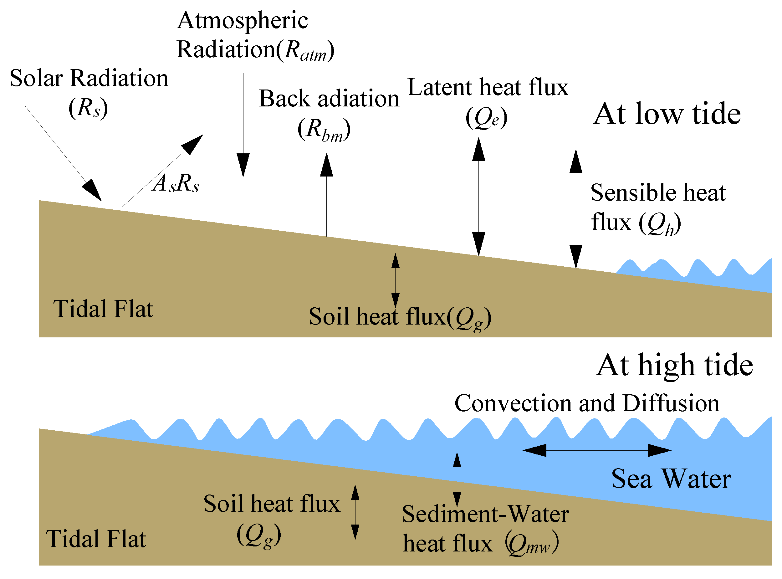
The tidal flat has two kinds of interfaces, the sediment-air interface and the sediment-water interface. Figure 1 gives the heat fluxes related to the two interfaces. If the water body is concerned, there is a greater air-water interface. Heat fluxes passing through the three interfaces include three kinds: Radiation based on no medium; latent heat transfer based on water movement among different states; and sensible heat after direct contacting.

Figure 1.
Schematic diagram of heat fluxes on the tidal flat.
(1) Solar Radiation Rs
Solar radiation is a short wave from sun, which is the main heat source of both tidal sediment and sea water. The energy of solar radiation cannot be wholly absorbed by sediment or water, some of which is reflected into the air. Thus, heat flux deduced by solar radiation is described as follows:
where: is the heat flux of solar radiation (W·m−2); is the albedo of the tidal sediment or sea water; C is fraction of sky covered by cloud (cloud cover); and a and b are coefficients. If solar radiation Rs data has been modified at the surface, the term about cloud cover in Equation (1) should be neglected. The albedo is not a constant, it changes with the angle of the sun and latitude. In addition, the heat flux of solar radiation is not absorbed only by the surface layer if the interface is the air-water condition. When the depth of water is shallow enough, some of the Q0 can reach the sediment-water surface, and the sediment can absorb the remaining energy. In this study, the solar radiation reaching the sediment’s surface is assumed to be negligible.
(2) Atmospheric Radiation Ratm and Back Radiation Rb
Atmospheric radiation and back radiation are all long wave radiation. Back radiation includes tidal sediment back radiation Rbm and sea water back radiation Rbw. According to the Stefan-Boltsmann’s law, the radiations can be calculated by the following formula:
where r is the reflection coefficient, and the subscript a represents air, m represents tidal sediment (mud), w represents sea water; ε is the emissivity factor; is the absolute temperature (K); σ is the Stefan-Boltzmann constant (5.6697 × 10⁻⁸ W·m−2·K−4); and g(C) is the function of cloud cover.
Equations (2)–(4) have a simple format, but a very complicated coefficient system, so the most commonly used formula is the effective back radiation formula:
where subscript L will be replaced by m for mud and w for water; QnetL is effective back radiation flux (W·m−2) of mud or water; ea is the vapor pressure (millibar) of the air; xi is coefficient, i = 1, 2, 3, 4; and n is index number.
Different scholars have offered different values of xi and n. Wyrtki [12] gives water formula coefficients xi as: 0.39, 0.05, 1.0, 0.5–0.8 (from equator to 70° of latitude), and n = 2. Delft3D-Flow gives n = 2 also, and xi as: 0.39, 0.058, 1.0, 0.65, but absolute temperature is replaced by . Kim uses n = 3.4, and the second term adopted the cloud cover modification, as well. The xi are 0.4, 0.05, 1.0, 0.75. The formula coefficients are the same for both sediment and water, and TL will be changed accordingly.
(3) Latent Heat Flux
The latent heat flux is mainly considered evaporative heat flux [13]. Here, the sediment-air interface is focused upon and the water-air interface will be discussed later.
where Qe is latent heat flux passed through sediment-air interface; ξw is the sediment porosity; ρa is the density of air (1.2929 kg·m−3) [11]; U is the wind speed (m·s−1); CV is the bulk transfer coefficient for evaporation (0.0014) [11]; qM is the specific humidity of saturated air, see the literature from Guarini et al. [11]; qa is the absolute air humidity; LV is the latent heat of evaporation (J·kg−1), which can be calculated by the following:
where TM(z0,t) is the sediment surface (Z0) temperature at time t (K).
(4) Sensible heat flux
The sensible heat flux of tidal sediment during exposure time can be calculated as follows:
where Qh is sensible heat flux passing through the sediment-air interface; CPa is the specific heat of air at constant pressure (1003.0 × 103 J·kg−1·K−1) [11]; and CH is the bulk transfer coefficient for conduction (0.0014) [11].
Under the inundation phase, the sensible heat flux passing through sediment-water interface can be described as:
where Qmw is sensible heat flux (W·m−2) passing through sediment-water interface; ksed is the sediment-water heat conductivity coefficient (W·m−1·K−1); and Hsed is the thickness of the sediment layer with significant heat exchanging.
There are three interfaces concerned in this study: they are the interfaces of air-sediment, air-water, and sediment-water. The sediment surface is unmovable, but the surface interface changes between the air-sediment interface and sediment-water interface due to the movement of tidal flow which usually has period of about 12.5 or 6 h. In addition, the solar radiation always has the period of about 12 h. The sun and tide movements with different periods will change the three interface conditions, it is difficult for scholars not majoring in meteorology to determine all the coefficients or factors accurately.
This study will focus on sediment-water heat exchange. The thermal state of the tidal sediment in different tide phases is important, so the sediment-air interface heat flux is concerned through some simplified coefficients. The water-air interface heat flux will be neglected, and a water temperature rise is adopted to replace the sea water temperature. This replacement can also avoid the open boundary temperature conditions which are varying after many factors that are difficult to be determined, as well.
2.2. Tidal Sediment Temperature Model
Temperature differences between the tidal sediment and sea water are the basic reason of heat exchange at sediment-water interface during flood time. Thus, temperature distribution of the tidal flat is needed in this study. According to the observed data from Tuller [14], Piccolo [15], Kim [10], Rinehimer [7], etc., the flat temperatures usually vary slightly in the horizontal direction, but significantly along the vertical direction, and a one-dimensional model can be simplified, as Kim [10] and Guarini et al. [11] had done.
The one-dimensional model for the temperature of tidal sediment is actually a solution of the one-dimensional heat conduction equation:
With:
where TM(z,t) is the sediment temperature (K) at the depth z; t is the time (s); α is the thermal diffusivity (m2·s−1) of the sediment [16,17]; Kz, ρM, and CPM are the heat conductivity (W·m−1·K−1), density (kg·m−3), and specific heat capacity (J·kg−3·K−1) of the mixture of sediment, interstitial water, and air.
Equation (10) can be discretized by the central difference scheme in space and matched implicit scheme in time. The depth z and the time t are labelled k, n, respectively. Φ=−(α·Δt)/(Δz)2, the discretization of the equation at the k layer is as follows:
where k = 2, 3, …, kmax − 1. The surface layer (k = 1) and the bottom layer (k = kmax) are needed to be limited separately.
The boundary conditions at the bottom layer are:
(1) No heat flux assumption:
(2) The given temperature process:
Boundary condition at the surface layer:
(1) Common module:
where Kz0 is the thermal conductivity (W·m−1·K−1), while ∂TM/∂z is the temperature gradient (°C·s−1) between the surface and subsurface sediment layers. The right terms of the different heat fluxes may not come out at the same time.
(2) The given temperature process:
Initial condition:
- (1)
- z ≤ 0.4 m,
- (2)
- 0.4 m < z ≤ 1.0 m,
The implicit difference from Equation (13) will be solved by the double sweep algorithm if both the first and end knots are well conditioned. Firstly, the field data reveals that the temperature varies very slightly at a certain point in the tidal flat, so the deep sediment layer can be set to a constant temperature during a time in days. The depth of the sediment layer is 1 m. Secondly, the solar radiation, air temperature, wind, cloud cover, and relative humidity are published by climate authorities weekly in China. These data can be adopted to calculate the sediment-air heat flux at the tidal flat surface.
2.3. Sea Water Temperature Rise Model
In coastal areas, the water body satisfies the assumption of the simplified horizontal two-dimensional model for violent vertical mixing. A 2D temperature rise numerical model can be established based on the 2D hydrodynamic model [18,19,20]. Here the orthogonal curvilinear grid hydrodynamic model equations are omitted, and the temperature rise transport equation as follows:
where ΔT is the temperature rise (°C); D is the total water column depth (m); (ξ, η) are the longitudinal and lateral directions of the grid under the orthogonal curvilinear coordinate; u and v are the velocity components in ξ and η directions; Cξ and Cη are the Lame coefficients in the orthogonal curvilinear coordinate; εξ and εη are the eddy diffusivity coefficients (m2·s−1); ρw is the density (1024 kg·m−3) of sea water; Cp is heat capacity (4186.8 J·kg−1·°C−1) of sea water; Ks is the heat loss coefficient (J·s−1·m−2·°C−1) from the water surface; and Qmw is the net heat flux (W·m−2) of sediment-water interface, by which the sediment temperature model is coupled into the 2D temperature rise model. The difference scheme of alternating direction implicit (ADI) was adopted, except that the discrete scheme of advection ΔT term is changed to the upwind scheme from the central scheme.
2.4. Study Area
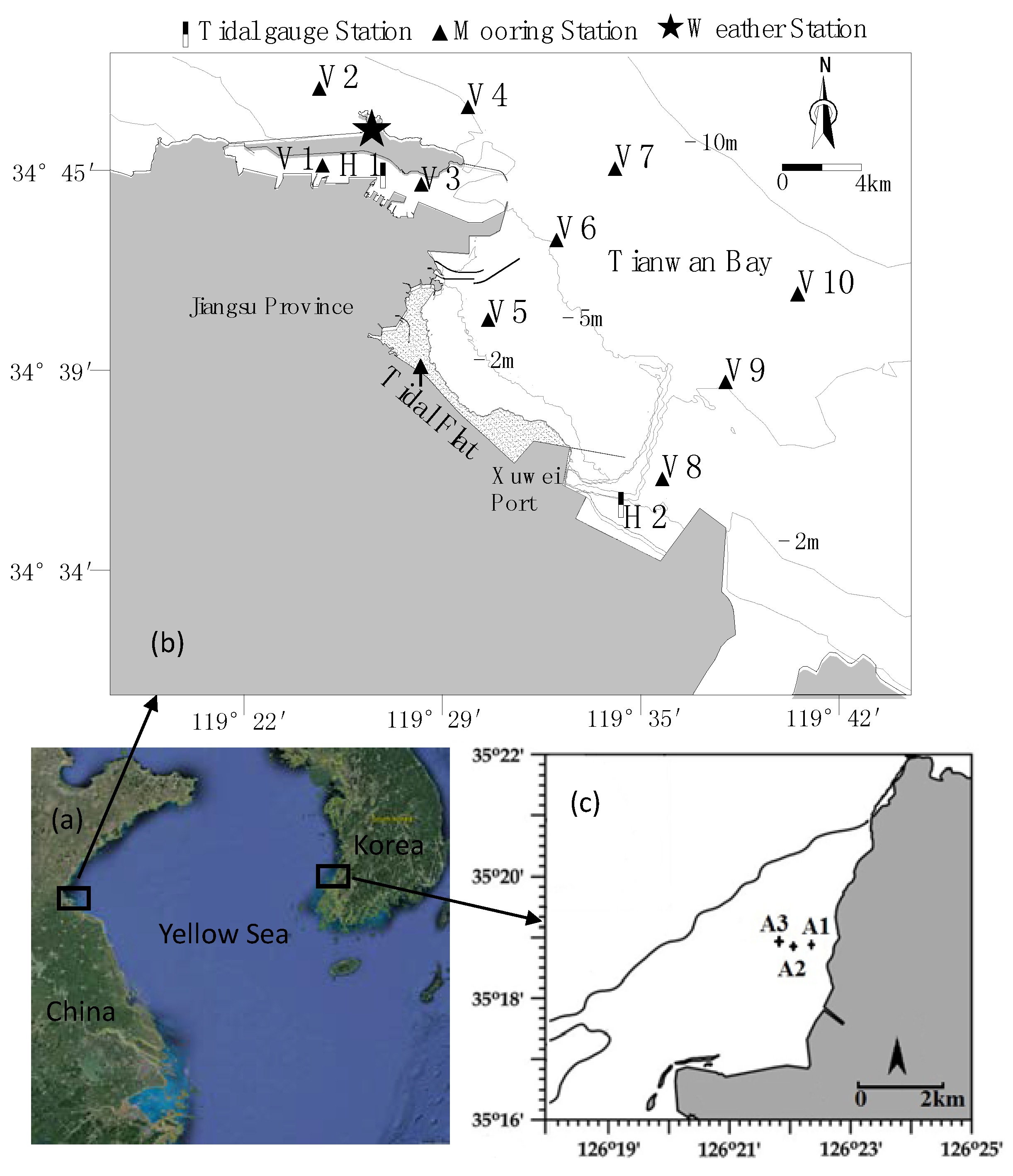
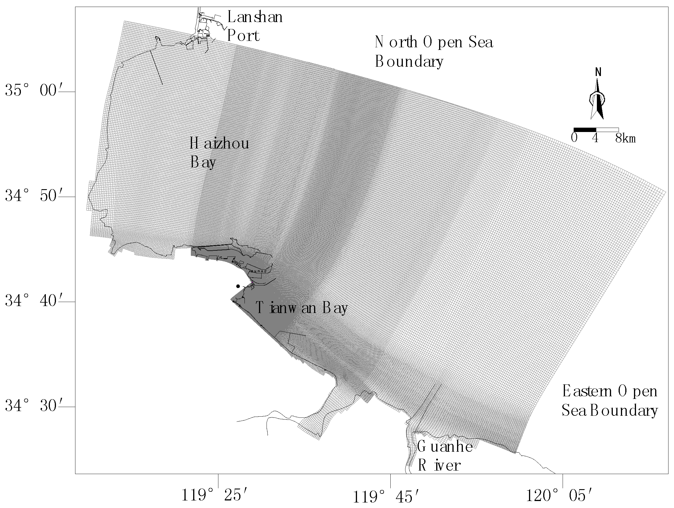
The study site was chosen from areas rich in marine topography, hydrodynamic observation, related climate factors, and sediment information for the coupled sediment temperature model. A relative stable tidal flat is welcomed, and big river mouth is avoided also. At last the Tianwan bay of Jiangsu province in China is chosen. The sketch of the studied bay is shown in Figure 2. There were ten stations for current mooring and two stations for tide gauges on 7–8 December 2010.

Figure 2.
Sketch of study site. (a) Map of the research areas in the eastern and western areas of the Yellow Sea; (b) Location of Tianwan Bay, China, bathymetry in meters, V1–V10 denote points of current mooring stations; H1 and H2 are points of tide gauges; (c) the Baeksu tidal flat in the western coast of Korea, A1–A3 are the three stations of sediment temperature.
Tianwan Bay is located on the west coast of the Yellow Sea. The shoreline of the study site is complicated. Some parts are developed as harbor, jetty, or groin, and the nature part is mainly distributed in the Tianwan Bay area. The slopes between two isobaths were 0.59° (1 m and 6 m), 0.04° (0 m and 1 m), 0.05° (−2 m and 0 m), and 0.03° (−5 m and −2 m), which were decreasing towards to sea. At low tide, its area is predominantly exposed as tidal flats, and covers an area of 15.8 km2 (the shadow area in Figure 2b) with a coastal length of about 13 km and a width of about 500 m to 2000 m. According to the long-term measurements (from 1951 to 2005), tides in the Jiangsu Province coastal area are dominated by a semidiurnal regular tide. The mean tidal range is 3.69 m. According to the long-term measurements (from 1960 to 2009), the annual mean temperature of the sea surface is 15.3 °C with a summer temperature of 20–26 °C and a winter temperature of 4–6 °C. The average air temperature is set to 14.5 °C and the relative humidity is set to 70%. The mean annual wind velocity is 5.5 m·s−1.
3. Model Calibration
3.1. The Calibration of Temperature Rise Model
Actually, the temperature rise model is difficult to calibrate, related calibrations are usually are tidal level, velocity, and current direction process verification, and sometimes the rationality of the Ks value will be checked.
An orthogonal curvilinear grid [21] was constructed using bathymetric data obtained from a number of surveys and Admiralty charts (Figure 3). The calculated area was 4526 km2. The domain extended for a distance of 89 km in the east–west direction and 33 km in the north–south direction with the calculated number of grids being 275 × 562. The horizontal grid spacing changed from 50 m in the near-shore area to 600 m at the open boundary. The time step was 20 s. The temporal processes of tidal levels at the open boundaries of hydrodynamic model were predicted using the harmonic constants over East China Sea [22]. The simulations of the model started from quiescent conditions (i.e., zero water velocities and a constant mean sea water level). The freezing method was adopted to deal with the moving boundary due to tidal waves at the tidal flat. The water depth at the grid node is used to determine whether the tidal flat is inundated or exposed. The water depth is used in the calculation directly when it is greater than the controlled water depth (5 cm). If not, the water level at the grid node is frozen and unchanged. The frozen water depth needs to be amended with the depth of the neighboring nodes for calculation of the next step.

Figure 3.
Study area: model domain and the orthogonal curvilinear grid.
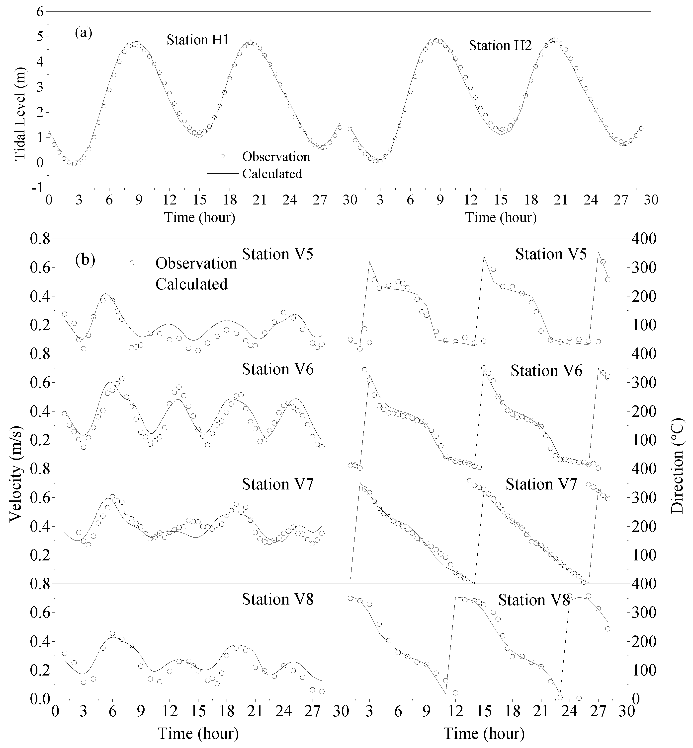
Part of the investigation process is given to compare with the simulated results in Figure 4. The simulated processes of the tide level are very close to the observed data. The tidal range is nearly 5 m, while the currents are very weak, the maximum of velocity is no more than 0.70 m/s. The correlation coefficient of the modeled versus observed velocity at station V5, V6, V7, and V8 are 0.75, 0.77, 0.70, and 0.80, respectively.
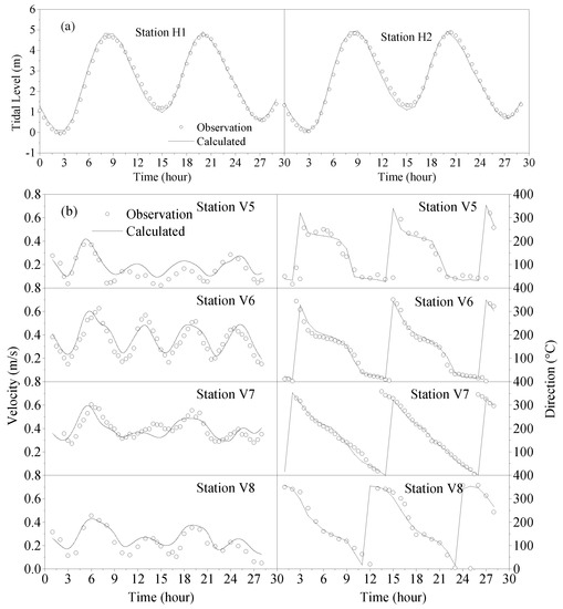
Figure 4.
Verification of hydrodynamics in the concerned area. (a) tidal levels; (b) current velocity and direction.
Ks is solved using the Gunneberg formula [23,24], which is relatively simple with respect to factors and easy to determine. Above all, the formula is welcomed for its long history in many places:
where Uz is wind speed (m·s−1) at z-m above the water surface, and Ts is the temperature (°C) of the water surface.
3.2. The Calibration of Sediment Temperature Model
The sediment temperature model cannot be verified at the study site for the lack of measured sediment temperature processes. Only Kim et al. [4,10] give enough field data for verifying the tidal sediment temperature model. This measurements were carried out in the Baesku tidal flat of the western Korean coast (Figure 2c) from 21 to 31 May 2003. The prediction of sediment temperature is essential for estimating the heat flux between the tidal sediment and seawater. Using these observed data, the tidal sediment temperature model is calibrated.
The temperature of the bottom sediment layer (end layer) is set to constant under the assumption of no heat flux at the layer. There are two purposes of this calibration. The first is to determine the thermal diffusivity α, and the second is to set a series of methods to determine the kinds of heat fluxes through the sediment surface.
The bulk of field observations have shown that thermal diffusivity varied with the sediment properties and water contents. The value of α is increasing from the surface to bottom, 0.33–0.64 × 10⁻⁶ m2·s−1, according to Kim’s literature [4]. These values are adopted to verify the model, and will be changed in Tianwan Bay’s study. Further discussion on the thermal diffusivity will be continued later.
Kim observed or collected data, including the temperature of sea water, tidal level, solar radiation, wind speed, air temperature and pressure, relative humidity, and cloud cover. These data are sufficient for calculating different heat fluxes at the sediment-air interface. During the inundation state, most of the heat fluxes at the sediment-water interface are neglected, except the sediment-water heat flux Qmw.
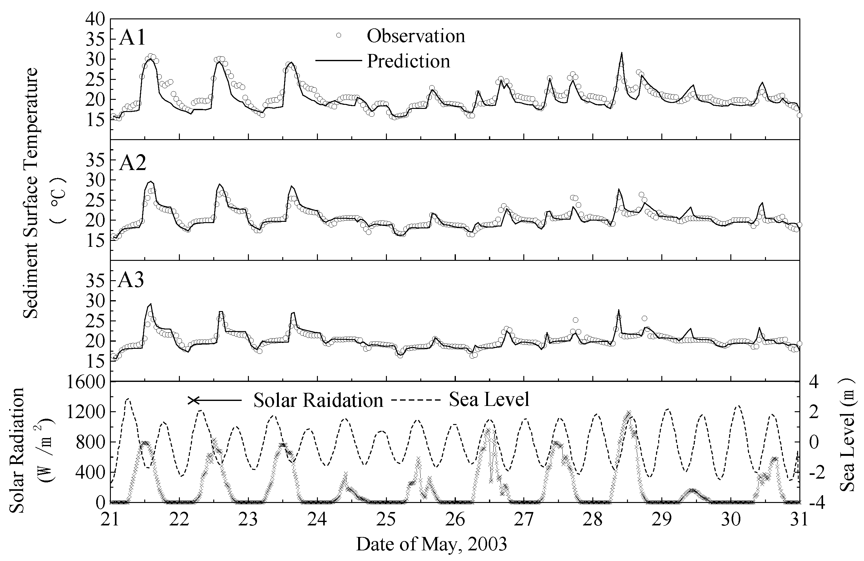
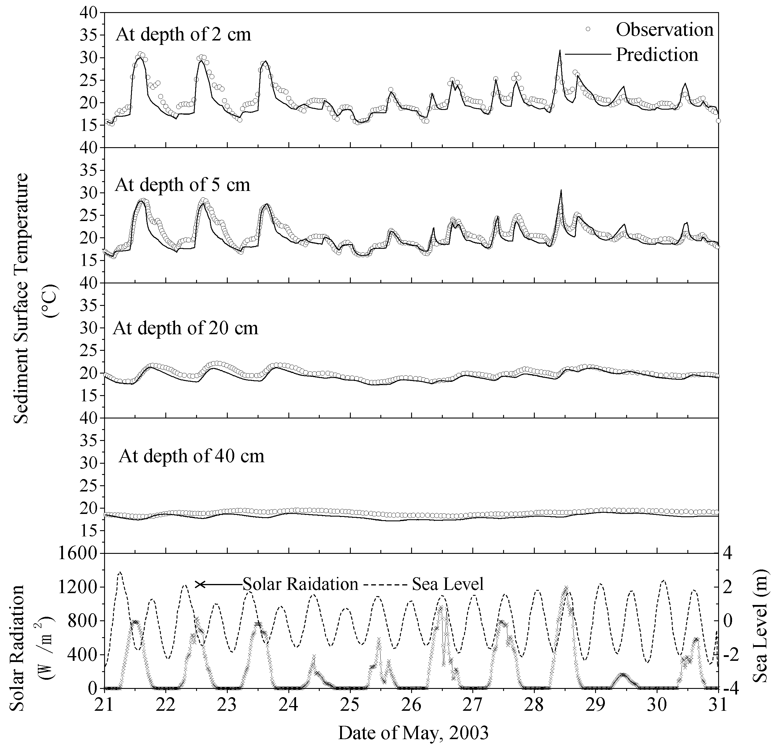
The sediment temperature model simulated five stations from 21 to 31 May 2003, Figure 5 shows a comparison between the observed and predicted temperatures of the sediment surface at three stations in the Beaku tidal flat. The model-predicted processes at the five stations matched well with the measured processes. The correlation coefficient (R2) between the measured and predicted temperatures exceeded 0.8 at stations B1, B2, and B3. During the inundation period, the variation in sediment surface temperature was well reproduced in the model at these stations. The observed and calculated temporal variations in the sediment temperature at each layer (2 cm, 5 cm, 20 cm, and 40 cm) at station A1 are shown in Figure 6. The temporal variations in the simulated sediment temperature agreed well with the observed temperature at each layer, with the correlation coefficient greater than 0.8. Therefore, it can be concluded from above comparisons that the model presented in this study is thus suitable for predicting the heat exchange between tidal sediments and seawater. In May, the sediment temperature in shallow tidal flat increased during the daytime and decreased during the night. The daily range of the sediment temperature in the shallow tidal flat was significantly larger than that in the lower layer (depth ≥ 20 cm), with the diurnal temperature variation in the sediment surface reaching 13.6 °C. Steep vertical temperature gradients developed within the shallow near-surface layers of the tidal flats when they were exposed, and the sediment temperature variation was of 6.5 °C within the first 0.05 m. Tidal flooding of the tidal flat resulted in isothermal or weakly thermal gradients.
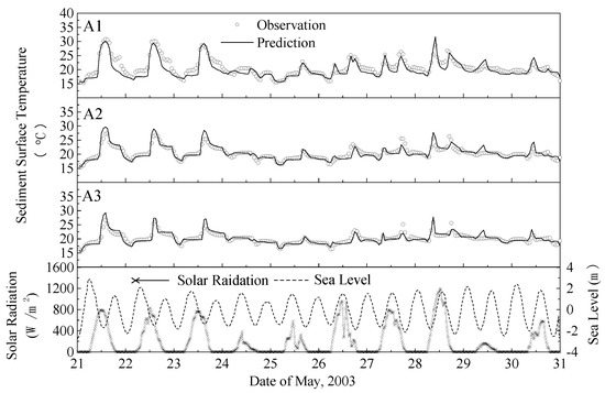
Figure 5.
Comparison between the observed and predicted temperatures of the 0.02 m depth at three stations in the Beaku tidal flat.

Figure 6.
The observed and calculated temporal variations in sediment temperature at each layer at station A1.
4. Case Study
During the model calibration study, thermal diffusivity in the sediment column has been adopted according to the field data. It is impossible for every study area to arrange field observation. Table 1 gives some information about the thermal coefficients and related sediment properties. It is a good reference for the preliminary value determination.

Table 1.
Overview of previous research about the thermal properties of tidal sediments.
It is indicated in Table 1 that the value of thermal diffusivity α has a positive correlation with the content of the sand in the sediment, and a negative correlation with the content of clay. The upper 0.15 m of the sediment in the study site is composed of coarse sand (2.1%), fine and medium sand (96.5%), and silty clay (1.4%). Thus, the thermal diffusivity may be greater than that of the verified site (from 0.33 × 10⁻⁶ to 1.06 × 10⁻⁶ m2·s−1). Three scenarios are set for thermal diffusivity α:
- (1)
- Scenario 1—from 0.33 × 10⁻⁶ to 1.06 × 10⁻⁶ m2·s−1
- (2)
- Scenario 2—from 0.40 × 10⁻⁶ to 1.27 × 10⁻⁶ m2·s−1 (positive deviation 20%)
- (3)
- Scenario 3—from 0.26 × 10⁻⁶ to 0.85 × 10⁻⁶ m2·s−1 (negative deviation 20%)
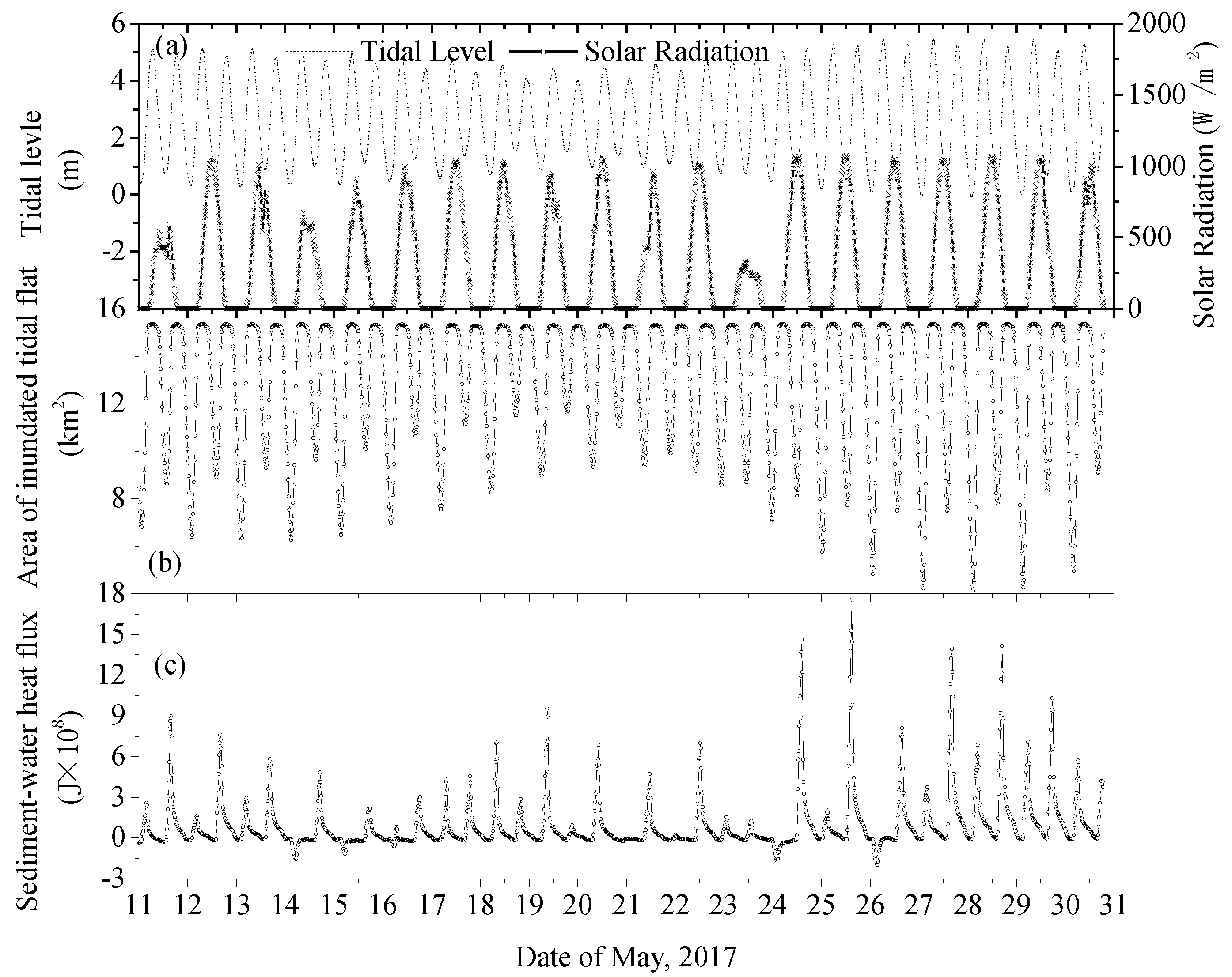
In the study site (Tianwan Bay), the climate data from 11 to 31 May 2017 were obtained from the China Meteorological Data Service Center (CMDC) [26]. The tidal level varies from −0.08 m to 5.5 m shown in Figure 7a, the areas of inundated tidal flats supplying heat flux of sediment-water are also shown in Figure 8b. The instant heat flux of sediment-water varies from −0.20 to 1.79 GJ/s (Scenario 1), positive value means heat flux from sediment to water while the negative one is the opposite. There are usually two different peaks every day, and the larger one always comes after noon; sometimes the peak value is negative when it comes in the early morning or later at night.
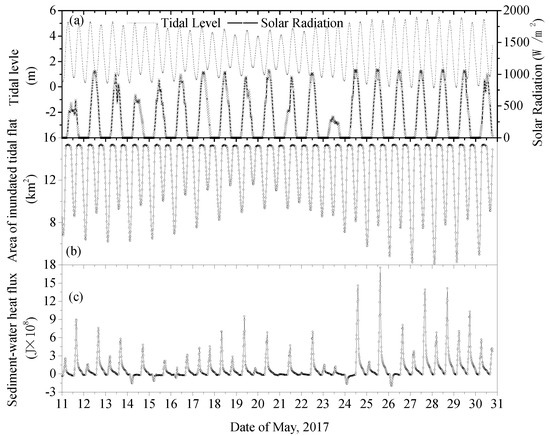
Figure 7.
The temporal process of (a) tidal level and solar radiation, (b) area of inundated tidal flats, and (c) sediment-water heat flux over 11–31 May 2017. The positive value indicates that heat flows from the sediment to the water, and the negative values indicate that heat flows from the water to the sediment.

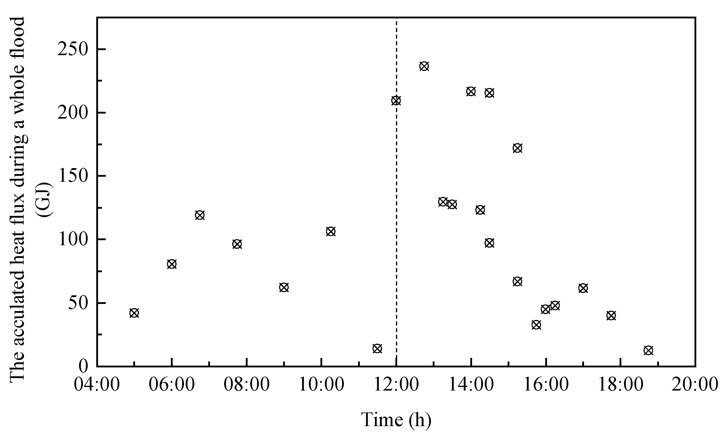
Figure 8.
The relationship between the timing of tidal inundation and the heat flux during a flooding period.
It can be found that the most important factor contributing to heat flux is not the area of inundation, but the time of inundating. If the inundated time begins at 1 p.m. to 3 p.m., the peak value is usually very high. Thus, the time of inundation is analyzed. Figure 8 shows the relationship between the timing of tidal inundation and the cumulative heat flux. The vertical axis represents the cumulative heat flux during a whole flood process, which is about 6 h. The horizontal axis shows the beginning time of inundation. The cumulative heat fluxes of the flood process are not the same even when the beginning times of inundation are very similar, because of the tidal ranges, the cloud covers, and solar radiations may all be different.
Figure 9 shows the total cumulative heat fluxes (TCHF) of the 20 days under different scenario conditions. Although the coefficients are different of each scenario, the differences of related values of cumulative heat fluxes are not very obvious. The TCHF in Scenario 1 is 2710.76 GJ from the tidal sediment to sea water. There is a trend that the greater the sediment diffusivity, the less heat is exchanged between the sediment-water interface. The thermal diffusivity of sediment is the coefficient of the efficient of heat transfer within the sediment column, the greater the value is, the faster the heat be transferred, and the less temperature of sediment surface will be during the exposure time. If the sediment diffusivity is set to a positive deviation of 20% (Scenario 2), the TCHF will be decreased by 5%, while a negative deviation of 20% (Scenario 3) will result in the TCHF increasing by about 6.5%. The variation of TCHF caused by the deviation of the sediment diffusivity is not significant. During the early study period, the value of sediment diffusivity should be reasonable rather than precise, taking into account the difficulties to determine it.
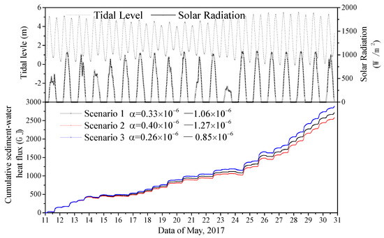
Figure 9.
Modeled time series of the cumulative heat fluxes for 11–31 May 2017 in the total tidal flat.
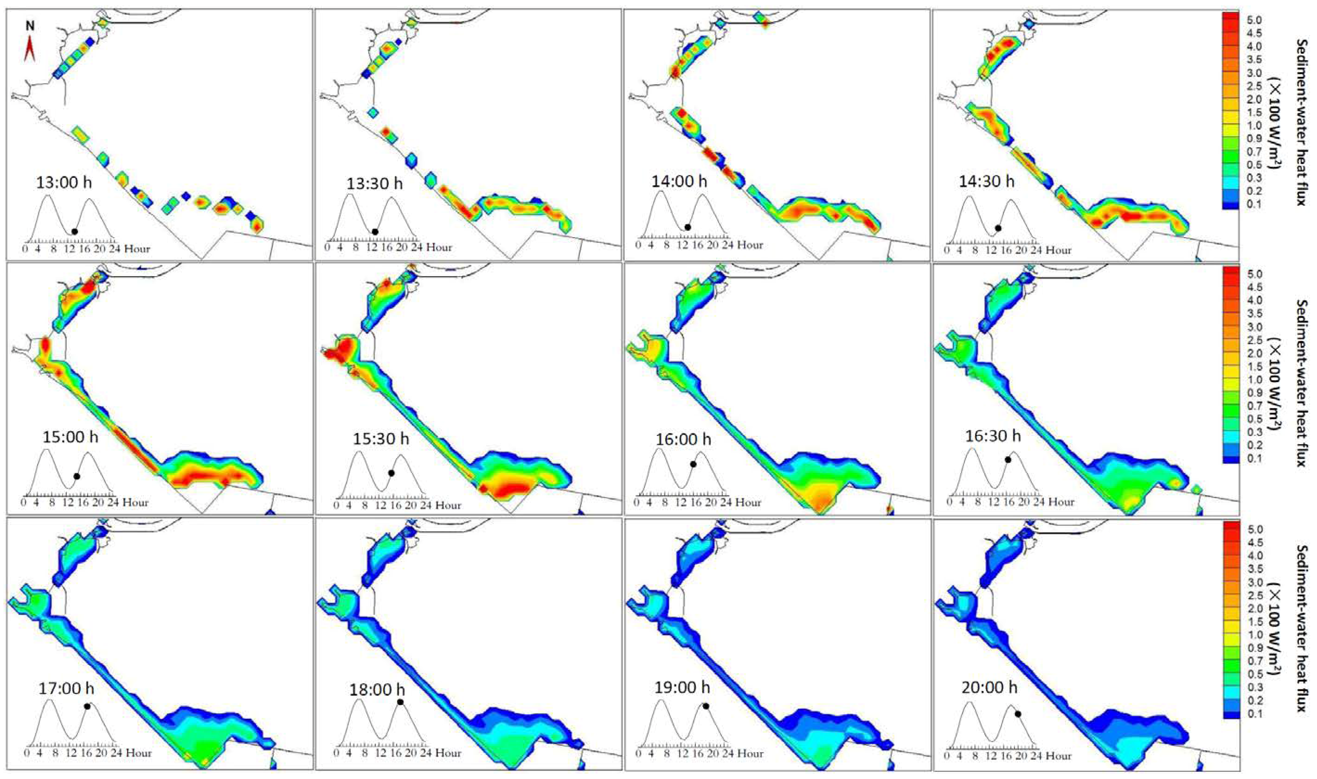
The heat exchange is further analyzed during the peak process of the whole calculated period. Figure 10 shows the distributions of sediment-water instantaneous heat fluxes at 12 different time moments with the same color-matching ruler to represent the whole flood process (second flood of 25 May). The time and tidal phase are shown in the left-down corner of each picture. It is clear that the flood tide began before 13:00 and reached flood slack around 18:00. Most of the red part (heat flux greater than 400 W/m2) comes between 14:00 and 15:30. After the tidal flat is inundated, the magnitude of heat flux is usually strong at the beginning and became smaller as the flooding lasted longer.
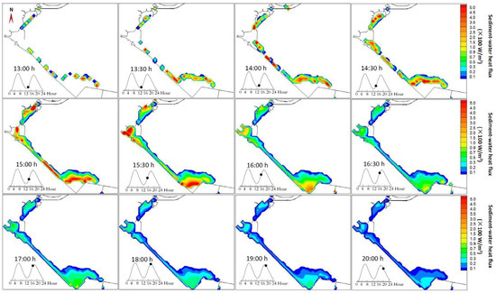
Figure 10.
The distributions of the sediment-water instantaneous heat fluxes at 12 different time moments on 25 May.
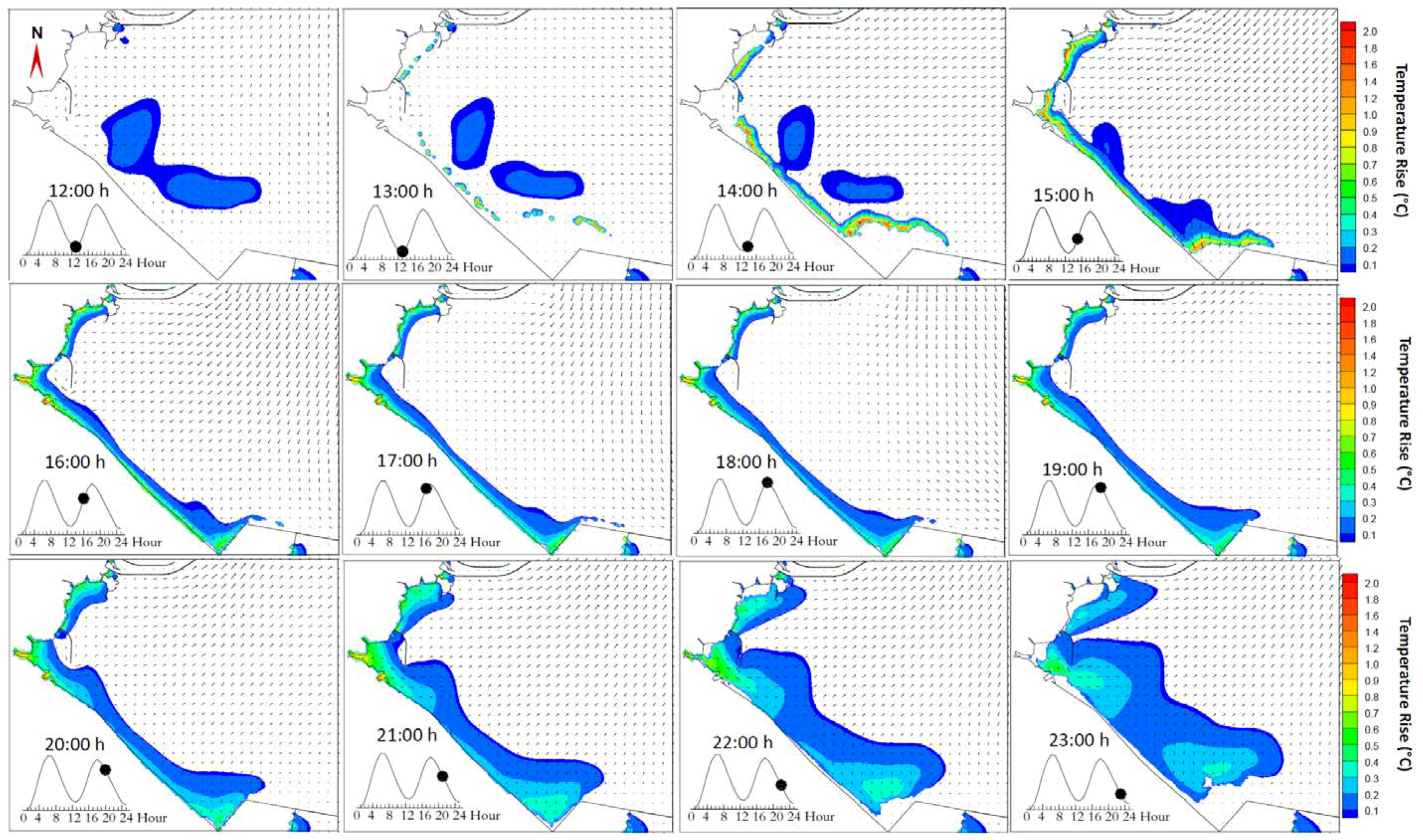
The temperature rise distribution of the water area is determined by both water depth and cumulative heat, locally. It is clear that the greater the depth is, the less the temperature rise will be. The more cumulative heat, the more the temperature rise will be. The heat exchanged from sediment to water will not stay in the local area for long. It will migrate with the flow, continue to spread into adjacent waters, and be lost through the water-air interface at the same time. Figure 11 shows the temperature rise of Tianwan bay during a whole flooding and ebbing tide process (the second tide process on 25 May). At the beginning, there is a peanut-shaped temperature rise area, which is the residual heat from the former period and will become smaller and smaller as the time proceeds (see the former three pictures). During the flooding period (pictures from 13 h to 18 h), the temperature rise area is narrowed and distributed in the area around the tidal front, while the temperature area spread into an obviously wider water area during the ebbing tide, but the enclosed area of the high temperature rise is getting smaller (in Table 2). The higher temperature rise (≥0.7 °C) often occurs during the first 3 h of the tidal inundation. During the flooding period, the areas of temperature rise decrease with the rising tidal level. The area of the lower temperature rise increases, and that of the higher temperature rise gradually disappears during the ebbing period. In a spring tide, the envelope areas of 0.5 °C and 1 °C reach 8.17 and 2.76 km2, respectively.
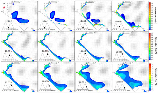
Figure 11.
The distributions of the temperature rise and flow field at 12 different time moments on 25 May.
Table 2.
The areas of seawater temperature rise caused by the sediment-water heat exchange.
5. Discussion
5.1. The Sediment Diffusivity
This study should still belong to the exploratory stage, as the values of many parameters depend on experience and historical data. Sediment diffusivity is the critical parameter in the sediment temperature model, which determines the temperature profile of the sediment column and heat fluxes of the interfaces of both sediment-water and sediment-air.
If the sediment is isotropic, the value of sediment diffusivity may be constant. However, the tidal flat is inundated by sea water periodically, and the water content should be varied along the vertical direction in a certain range. The studied sediment column is actually the mixture of water and sediment. Properties of this mixture are affected by water content, and sediment diffusivity can be an exception. Thus, a reasonable method to determine the sediment diffusivity should at least be based on the properties of both sediment and water content. It will be a complicated process to determine all these properties in an actual tidal flat, as scouring and silting may happen.
A group of analyzed values of sediment diffusivity based on a large amount of field data are adopted in this study. This usage is to avoid some unexpected errors. The values of sediment diffusivity in Tianwan tidal flat are surely different with those of the Beaksu tidal flat. Thus, a deviation of ±20% of sediment diffusivity is simulated to check its sensibility. The variation of total cumulative heat fluxes caused by the deviation of sediment diffusivity is not significant. This is a pleasant result, so the primary study can continue based on these values of sediment diffusivity.
5.2. Coefficient of Heat Loss from the Water Surface
The temperature rise model has simplified conditions and parameters related to both open boundary and water-air interface. Thus, the coefficient of heat loss from the water surface (Ks) may be the most important factor in the temperature rise model.
The Gunneberg formula is adopted to determine Ks, which is influenced only by water temperature and wind. The differences between day and night may weaken. The temperature of the air during the simulating period varies from 16 to 34.8 °C. The heat loss during the night may be overestimated. Thus, the total cumulative heat fluxes may be underestimated, as well as the temperature rise area.
A real water temperature model will be surely developed in the future. The simplified temperature rise model is still useful in the present stage, especially when the heat exchange between water and sediment is not very clear.
In this study, we focus on the summer months’ condition and reveal the importance of the sediment-water heat exchange on seawater temperature. Due to the different direction of sediment-water heat flux between the summer season and the winter season, the next step is to research the influence of the tidal sediment heat transfer on seawater temperature under winter condition. In addition, the heat transfer capacity of the tidal sediment is affected by many thermodynamic parameters. Thus, the effect of the tidal sediment’s thermodynamic properties difference on the seawater temperature is necessary in further studies.
6. Conclusions
This work simulates the dispersion of a temperature rise caused by the influence of a sediment-water heat exchange. A module, which was used to calculate the sediment-water heat flux, was added into the numerical model of the seawater temperature rise to achieve the heat exchange between the seabed and water in the tidal zone. The model was first calibrated based on the measured hydrodynamic data and the collected temperature data of the tidal sediment. The calibrated model was then used to simulate the distribution of temperature rise.
Results show that the temperature of seawater is evidently influenced by the sediment-water heat exchange. The tidal sediment is as a heat source providing heat to seawater. The magnitude of the sediment-water heat flux primarily depends on the timing of the tidal inundation. The maximum instantaneous heat flux is 1.76 × 10⁸ J with 14 km2 of inundated tidal flat. The cumulative net heat flux is 2710 GJ over the 20-day period. In a spring tide cycle, the temperature rise can reach 2 °C in the local area, and the envelope areas of 0.5 °C and 1 °C temperature rises are 8.17 and 2.76 km2, respectively. This model is a useful tool for ecosystem evaluation in the tidal flat or near-shore water area.
Author Contributions
J.M. and Y.G. conceived and designed the model; and Y.G. conducted the model application, wrote and revised the paper.
Funding
This research was funded by “National Key Research and Development Program of China” grant number “2017YFC0405504”, and “National Natural Science Foundation of China’ grant number “51609152”.
Conflicts of Interest
The authors declare no conflict of interest.
References
- Cech, J.J.; Mitchell, S.J.; Castleberry, D.T.; Mcenroe, M. Distribution of California stream fishes: Influence of environmental temperature and hypoxia. Environ. Biol. Fishes 1990, 29, 95–105. [Google Scholar] [CrossRef]
- Verones, F.; Hanafiah, M.M.; Pfister, S.; Huijbregts, M.A.; Pelletier, G.J.; Koehler, A. Characterization factors for thermal pollution in freshwater aquatic environments. Environ. Sci. Technol. 2010, 44, 9364–9368. [Google Scholar] [CrossRef] [PubMed]
- Wither, A.; Bamber, R.; Colclough, S.; Dyer, K.; Elliott, M.; Holmes, P.; Jenner, H.; Taylor, C.; Turnpenny, A. Setting new thermal standards for transitional and coastal (TraC) waters. Mar. Pollut. Bull. 2012, 68, 46–50. [Google Scholar] [CrossRef] [PubMed]
- Kim, T.W.; Cho, Y.K. Calculation of heat flux in a macrotidal flat using FVCOM. J. Geophys. Res. Oceans 2011, 116, 869–881. [Google Scholar] [CrossRef]
- Masahiro, S.; Masumi, K.; Katumi, Y.; Fumiya, T. Heat and temperature environments at the muddy tidal flat in the interior parts of the Ariake Sea and its effects on bioturbation. J. Coast. Eng. 2009, 65, 1136–1140. [Google Scholar]
- Vugts, H.F.; Zimmerman, J.T.F. Heat balance of a tidal flat area. Neth. J. Sea Res. 1985, 19, 1–14. [Google Scholar] [CrossRef]
- Rinehimer, J.P.; Thomson, J.T. Observations and modeling of heat fluxes on tidal flats. J. Geophys. Res. Oceans 2014, 119, 133–146. [Google Scholar] [CrossRef]
- Harrison, S.J.; Phizacklea, A.P. Vertical temperature gradients in muddy intertidal sediments in the Forth estuary, Scotland. Limnol. Oceanogr. 1987, 32, 954–963. [Google Scholar] [CrossRef]
- Kim, T.W.; Cho, Y.K. Heat flux across the surface of a macrotidal flat in southwest Korea. J. Geophys. Res. 2009, 114, 1748–1755. [Google Scholar] [CrossRef]
- Kim, T.W.; Cho, Y.K.; You, K.W.; Jung, K.T. Effect of tidal flat on seawater temperature variation in the southwest coast of Korea. J. Geophys. Res. 2010, 115, 526–534. [Google Scholar] [CrossRef]
- Guarini, J.M.; Blanchard, G.F.; Gros, P.; Harrison, S.J. Modelling the mud surface temperature on intertidal flats to investigate the spatio-temporal dynamics of the benthic microalgal photosynthetic capacity. Mar. Ecol. Prog. Ser. 1997, 153, 25–36. [Google Scholar] [CrossRef]
- Wyrtki, K. The average annual heat balance of the North Pacific Ocean and its relation to ocean circulation. J. Geophys. Res. 1965, 70, 4547–4559. [Google Scholar] [CrossRef]
- Cuceloglu, G.; Abbaspour, K.; Ozturk, I. Assessing the Water-Resources Potential of Istanbul by Using a Soil and Water Assessment Tool (SWAT) Hydrological Model. Water 2017, 9, 814. [Google Scholar] [CrossRef]
- Tuller, S.E. Energy balance microclimatic variations on a coastal beach. Tellus 1972, 24, 260–270. [Google Scholar] [CrossRef]
- Piccolo, M.C.; Perillo, G.M.E.; Daborn, G.R. Soil Temperature Variations on a Tidal Flat in Minas Basin, Bay of Fundy, Canada. Estuar. Coast. Shelf Sci. 1993, 36, 345–357. [Google Scholar] [CrossRef]
- Miao, Y.C.; Liu, S.H.; Lu, S.H.; Zhang, Y. A comparative study of computing methods of soil thermal diffusivity, temperature and heat flux. Chin. J. Geophys. 2012, 55, 441–451. [Google Scholar] [CrossRef]
- Thomson, J.M. Observations of thermal diffusivity and a relation to the porosity of tidal flat sediments. Agric. Meteorol. 2010, 115, C05016. [Google Scholar] [CrossRef]
- Ma, J.R.; Zhang, X.Y.; Zhang, X.N. Thermal buoyancy effect in two-dimensional cooling water mathematical models. Hydro-Sci. Eng. 2005, 3, 37–40. [Google Scholar]
- Ma, J.R.; Guo, Y.Q.; Zou, G.L. Analysis on changes of flow and sediment characteristic caused by Jiaojiang River control works. Yangtze River 2013, 44, 85–89. [Google Scholar]
- Ma, J.R.; Guo, Y.Q.; Yao, L. Flow condition and engineering measures of lanqiao jetty and oil dock area in Lanshan harbor of Rizhao port. Ocean Eng. 2010, 28, 127–131. [Google Scholar]
- Durán-Colmenares, A.; Barrios-Piña, H.; Ramírez-León, H. Numerical Modeling of Water Thermal Plumes Emitted by Thermal Power Plants. Water 2016, 8, 482. [Google Scholar] [CrossRef]
- Song, Z.Y.; Yan, Y.X.; Mao, L.H. A tidal harmonious analysis method. Ocean Eng. 1997, 15, 40–45. [Google Scholar]
- Gunneberg, F. Probleme bei der Berechnung des Warmeaustauches Gewasser/Atmoshpare. Warmeeinleitungen in Gewasser und Deren Auswirkungen; Die Abwarme Kommission Geschaftsstelle beim Umweltbundesamt: Berlin, Germany, 1987. [Google Scholar]
- Zhang, S.N.; Tong, L. Experimental study on the heat loss coefficient from water surface in laboratory. Water Resour. Prot. 1986, 2, 1059–1067. [Google Scholar]
- Losordo, T.M.; Piedrahita, R.H. Modelling temperature variation and thermal stratification in shallow aquaculture ponds. Ecol. Model. 1991, 54, 189–226. [Google Scholar] [CrossRef]
- China Meteorological Data Service Center. Available online: http://data.cma.cn/en/?r=site/index (accessed on 7 June 2017).

© 2018 by the authors. Licensee MDPI, Basel, Switzerland. This article is an open access article distributed under the terms and conditions of the Creative Commons Attribution (CC BY) license (http://creativecommons.org/licenses/by/4.0/).