Performance of National Maps of Watershed Integrity at Watershed Scales

 , , , , , , ,
  , ,
, ,
Abstract
:
1. Introduction
2. Materials and Methods
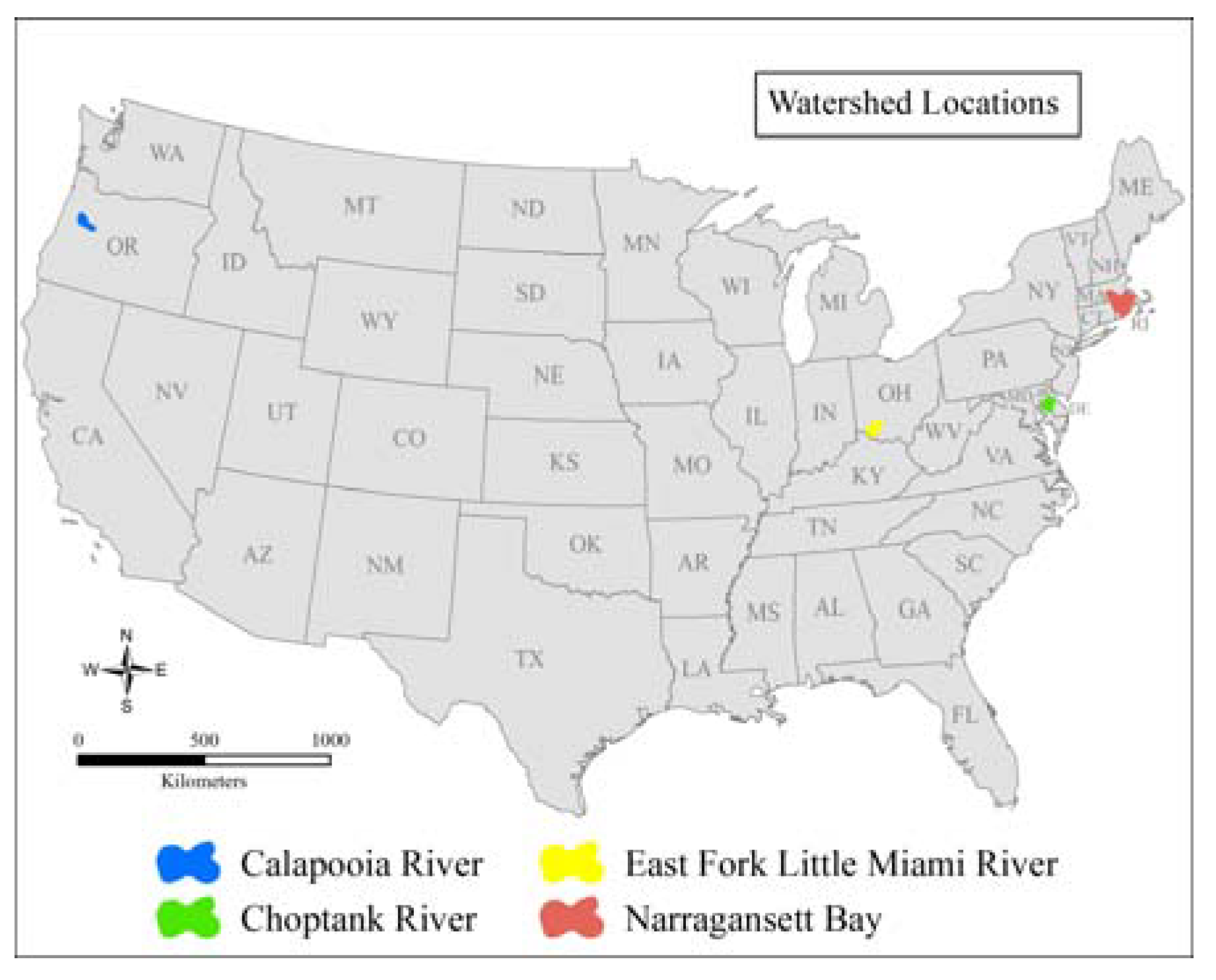
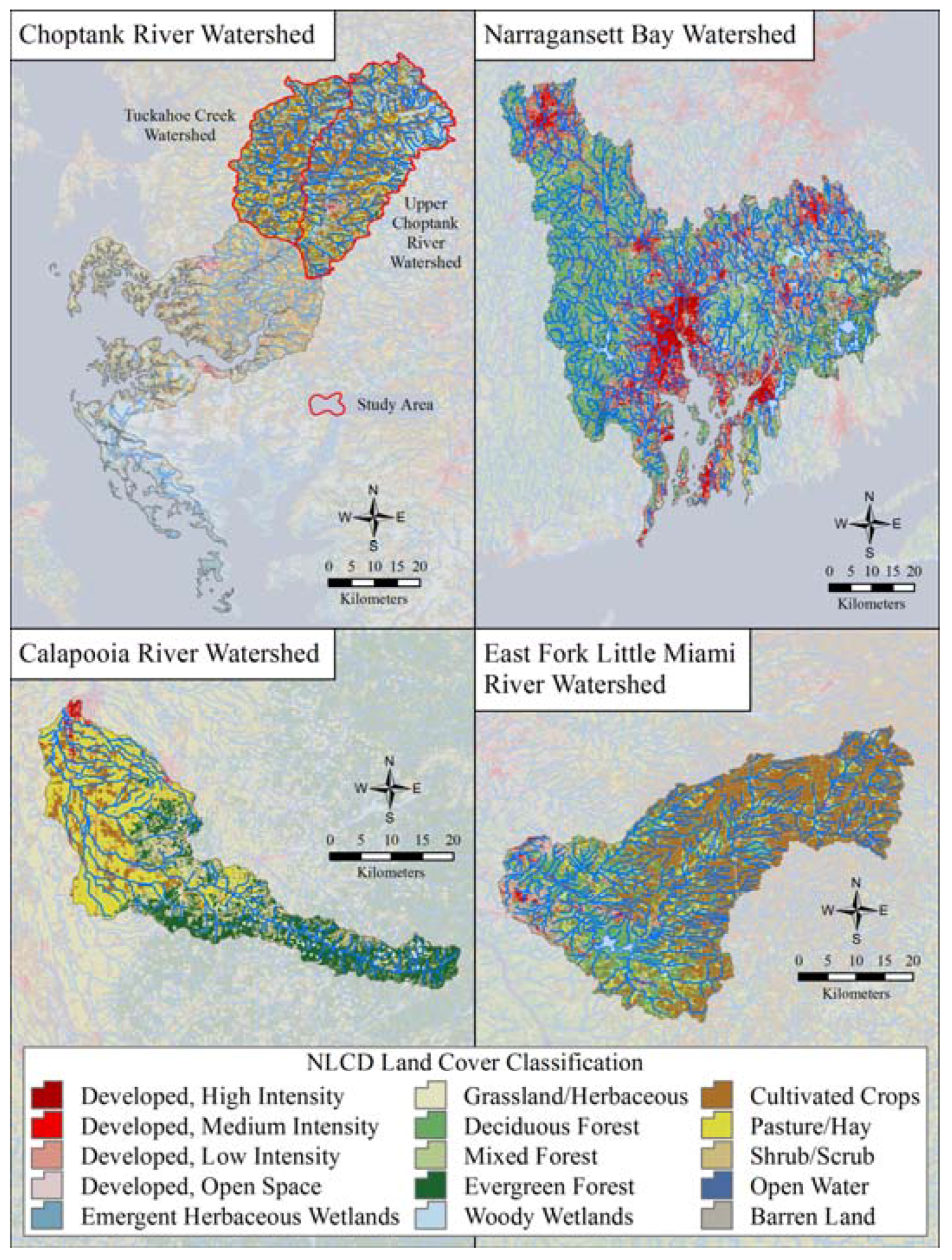
2.1. Study Areas
2.1.1. Calapooia River Watershed
2.1.2. Choptank Study Area: Upper Choptank River and Tuckahoe Creek Sub-Basins
2.1.3. East Fork Little Miami River Watershed
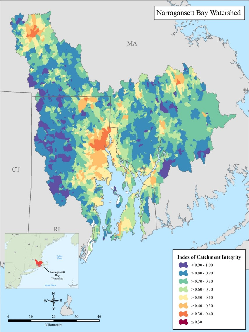
2.1.4. Narragansett Bay Watershed
2.2. Case Study Response Variables
2.2.1. Calapooia River Watershed
2.2.2. Choptank Study Area: Upper Choptank River and Tuckahoe Creek Sub-Basins
2.2.3. East Fork Little Miami River Watershed
2.2.4. Narragansett Bay Watershed
Stream Chemistry
Stable Isotope Ratios of δ15N and δ13C for Periphyton
Stable Isotope Ratios of δ15N and δ13C for Benthic Organic Matter in Lakes
2.3. Explanatory Predictor Variables
2.4. Statistical Analyses
3. Results
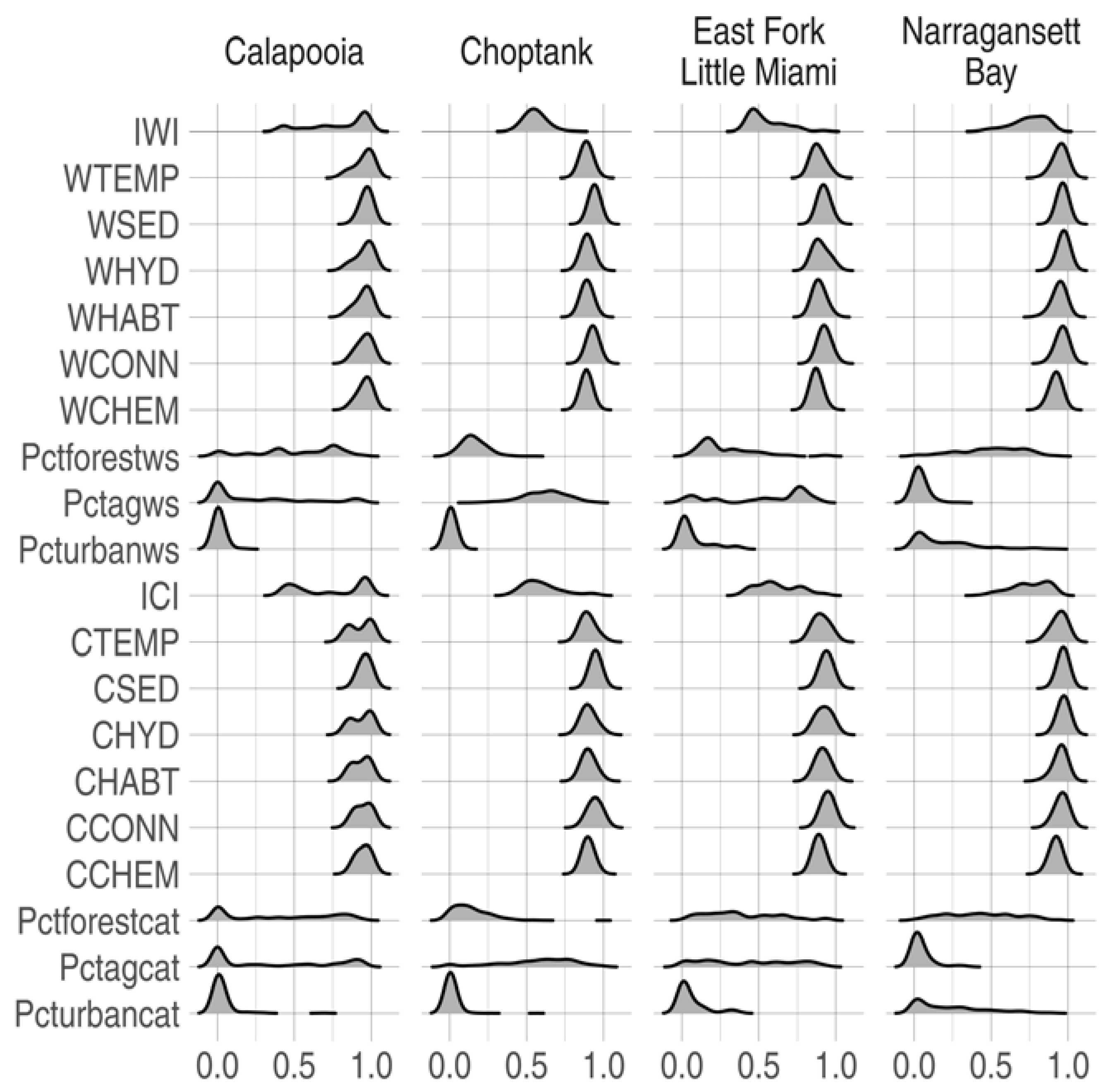
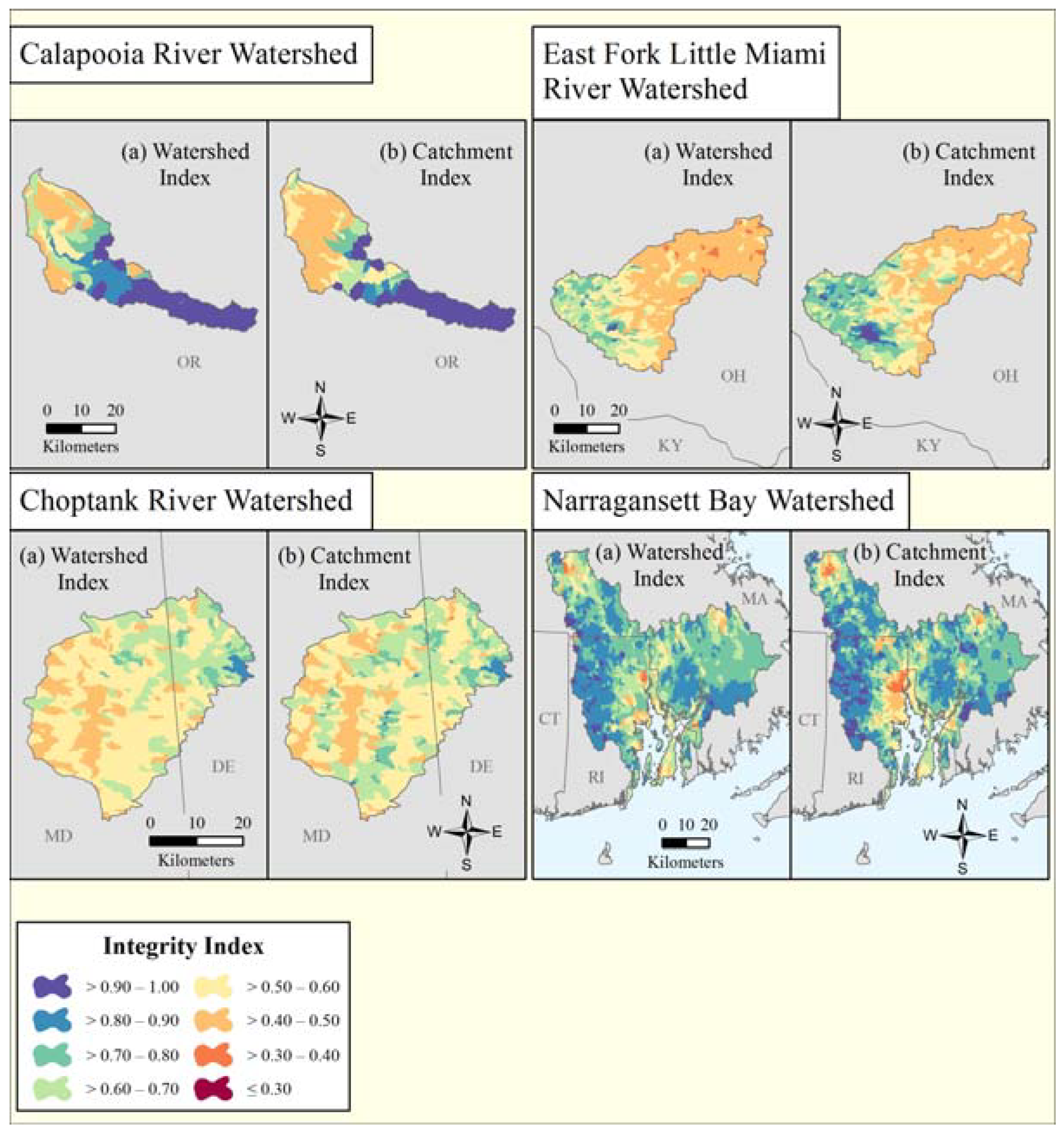
3.1. Indices of Watershed and Catchment Integrity
3.2. Correlations with IWI/ICI Values Across Case Study Watersheds
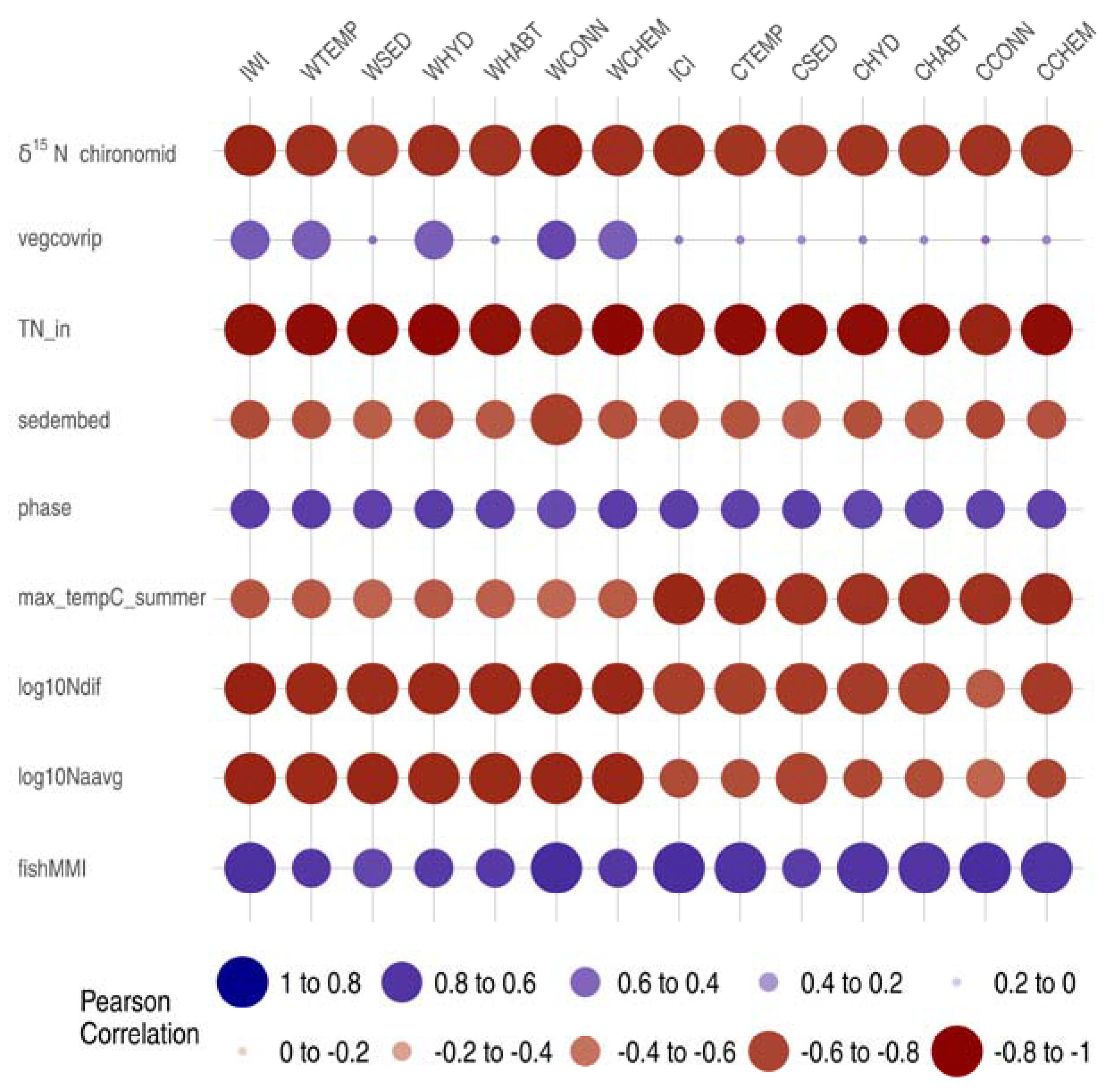
3.2.1. Calapooia River Watershed
3.2.2. Choptank Watershed
3.2.3. East Fork Little Miami River Watershed
3.2.4. Narragansett Bay Watershed
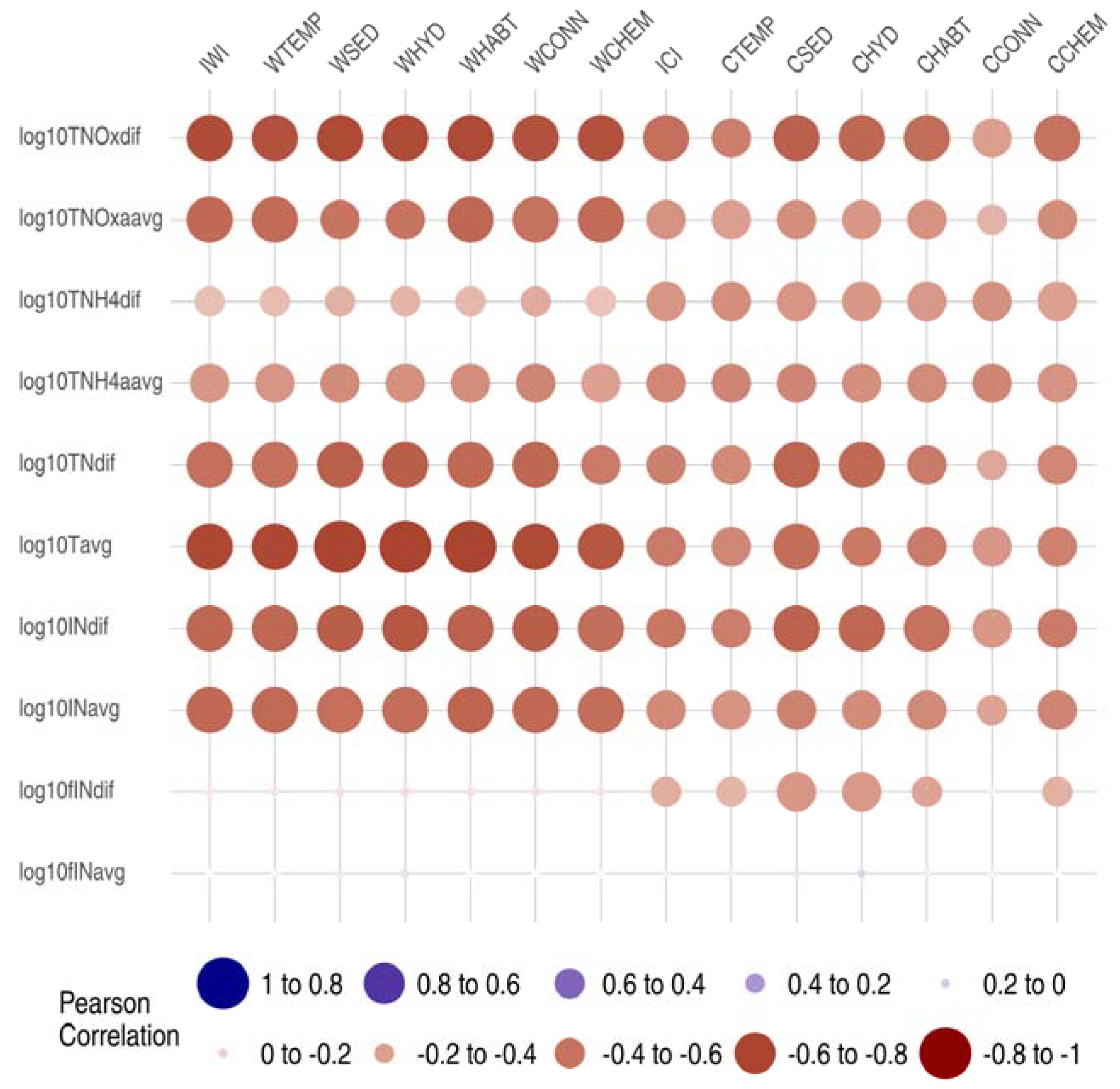
3.3. Correlations with Landscape Explanatory Variables Across Case Study Watersheds
4. Discussion
5. Conclusions
Supplementary Materials
Author Contributions
Acknowledgments
Conflicts of Interest
References
- U.S. Environmental Protection Agency (EPA). Healthy Watersheds Initiative: National Framework and Action Plan; Publication Number: EPA 841-R-11-005; Environmental Protection Agency (EPA): Washington, DC, USA, 2011.
- Flotemersch, J.E.; Leibowitz, S.G.; Hill, R.A.; Stoddard, J.L.; Thoms, M.C.; Tharme, R.E. A Watershed Integrity Definition and Assessment Approach to Support Strategic Management of Watersheds. River Res. Appl. 2016, 32, 1654–1671. [Google Scholar] [CrossRef]
- Millennium Ecosystem Assessment. Ecosystems and Human Well-Being: Synthesis; Island Press: Washington, DC, USA, 2005. [Google Scholar]
- Costanza, R.; d’Arge, R.; De Groot, R.; Faber, S.; Grasso, M.; Hannon, B.; Limburg, K.; Naeem, S.; O’Neill, R.V.; Paruelo, J.; et al. The Value of the World’s Ecosystem Services and Natural Capital. Nature 1997, 387, 253–260. [Google Scholar] [CrossRef]
- Costanza, R.; de Groot, R.; Sutton, P.; van der Ploeg, S.; Anderson, S.J.; Kubiszewski, I.; Farber, S.; Turner, R.K. Changes in the Global Value of Ecosystem Services. Glob. Environ. Chang. 2014, 26, 152–158. [Google Scholar] [CrossRef]
- De Groot, R.S.; Wilson, M.A.; Boumans, R.M.J. A Typology for the Classification, Description and Valuation of Ecosystem Functions, Goods and Services. Ecol. Econ. 2002, 41, 393–408. [Google Scholar] [CrossRef]
- Poff, N.L.; Allan, J.D.; Bain, M.B.; Karr, J.R.; Prestegaard, K.L.; Richter, B.D.; Sparks, R.E.; Stromberg, J.C. The Natural Flow Regime. Bioscience 1997, 47, 769–784. [Google Scholar] [CrossRef]
- Allan, J.D. Landscapes and Riverscapes: The Influence of Land Use on Stream Ecosystems. Annu. Rev. Ecol. Evol. Syst. 2004, 35, 257–284. [Google Scholar] [CrossRef]
- Thoms, M.C.; Parsons, M.E.; Foster, J.M. The Use of Multivariate Statistics to Elucidate Patterns of Floodplain Sedimentation at Different Spatial Scales. Earth Surf. Process. Landf. 2007, 32, 672–686. [Google Scholar] [CrossRef]
- U.S. Environmental Protection Agency (EPA). Safe and Sustainable Water Resources: Strategic Research Action Plan 2012–2016; U.S. Environmental Protection Agency: Washington, DC, USA, 2012.
- U.S. Environmental Protection Agency (EPA). National Rivers and Streams Assessment 2008–2009 Technical Report; U.S. Environmental Protection Agency, Office of Wetlands, Oceans and Watersheds and Office of Research and Development: Washington, DC, USA, 2016. Available online: https://www.epa.gov/sites/production/files/2016-03/documents/nrsa_08_09_technical_appendix_03082016.pdf (accessed on 1 May 2018).
- Flotemersch, J.E.; Stribling, J.B.; Paul, M.J. Concepts and Approaches for the Bioassessment of Non-Wadeable Streams and Rivers; EPA/600/R-06/127; U.S. Environmental Protection Agency: Cincinnati, OH, USA, 2006.
- Hill, R.A.; Weber, M.H.; Leibowitz, S.G.; Olsen, A.R.; Thornbrugh, D.J. The Stream-Catchment (Streamcat) Dataset: A Database of Watershed Metrics for the Conterminous United States. J. Am. Water Resour. Assoc. 2016, 52, 120–128. [Google Scholar] [CrossRef]
- Wang, G.; Mang, S.; Haisheng, C.; Liu, S.; Zhang, Z.; Wang, L.; Innes, J.L. Integrated watershed management: Evolution, development and emerging trends. J. For. Res. 2016, 27, 967–994. [Google Scholar] [CrossRef]
- Megdal, S.B.; Eden, S.; Shamir, E. Water governance, stakeholder engagement, and sustainable water resources management. Water 2017, 9, 190. [Google Scholar] [CrossRef]
- Voulvoulis, N.; Arpon, K.D.; Giakoumis, T. The EU Water Framework Directive: From great expectations to problems with implementation. Sci. Total Environ. 2017, 575, 358–366. [Google Scholar] [CrossRef] [PubMed]
- Karr, J.R. Ecological integrity and ecological health are not the same. In Engineering within Ecological Constraints; Schulze, P., Ed.; National Academy of Science: Washington, DC, USA, 1996; pp. 97–110. ISBN 0-309-05198-3. [Google Scholar]
- Noss, R.F. Some suggestions for keeping national wildlife refuges healthy and whole. Nat. Resour. J. 2004, 44, 1093–1111. [Google Scholar]
- Allan, J.D.; Castillo, M.M. Stream Ecology: Structure and Function of Running Waters; Springer: Dordrecht, The Netherlands, 2007; ISBN 978-1-4020-5582-9. [Google Scholar]
- Kwak, T.J.; Freeman, M.C. Assessment and management of ecological integrity. In Inland Fisheries Management in North America, 3rd ed.; Hubert, W.A., Quist, M.C., Eds.; American Fisheries Society: Bethesda, MD, USA, 2010; pp. 353–394. [Google Scholar]
- Jordan, S.J.; Benson, W.H. Sustainable Watersheds: Integrating ecosystem services and public health. Environ. Health Insights 2015, 9, 1–7. [Google Scholar] [CrossRef] [PubMed]
- Kim, J.Y.; An, K.G. Integrated ecological river health assessments, based on water chemistry, physical habitat quality and biological integrity. Water 2015, 7, 6378–6403. [Google Scholar] [CrossRef]
- Vörösmarty, C.J.; McIntyre, P.B.; Gessner, M.O.; Dudgeon, D.; Prusevich, A.; Green, P.; Glidden, S.; Bunn, S.E.; Sullivan, C.A.; Liermann, C.R.; et al. Global threats to human water security and river biodiversity. Nature 2010, 467, 555–561. [Google Scholar] [CrossRef] [PubMed]
- Thornbrugh, D.J.; Leibowitz, S.G.; Hill, R.A.; Weber, M.H.; Johnson, Z.C.; Olsen, A.R.; Flotemersch, J.E.; Stoddard, J.L.; Peck, D.V. Mapping watershed integrity for the conterminous United States. Ecol. Indic. 2018, 85, 1133–1148. [Google Scholar] [CrossRef] [PubMed]
- U.S. Census Bureau. Decennial Census of Population and Housing. Washington, DC, USA, 2010. Available online: https://www.census.gov/programs-surveys/decennial-census/decade.2010.html (accessed on 18 April 2017).
- Pacific Northwest Ecosystem Research Consortium. Willamette Valley Planning Atlas; Oregon State University Press: Corvallis, OR, USA, 2002. [Google Scholar]
- McCarty, G.W.; McConnell, L.L.; Hapeman, C.J.; Sadeghi, A.; Graff, C.; Hively, W.D.; Lang, M.W.; Fisher, T.R.; Jordan, T.; Rice, C.P.; et al. Water quality and conservation practice effects in the Choptank River watershed. J. Soil Water Conserv. 2008, 63, 461–474. [Google Scholar] [CrossRef]
- Tiner, R.W.; Burke, D.G. Wetlands of Maryland; U.S. Fish and Wildlife Service: Hadley, MA, USA; Maryland Department of Natural Resources (Cooperative Publication): Annapolis, MD, USA, 1995; p. 193.
- Ator, S.; Denver, J.; Krantz, D.; Newell, W.; Martucci, S. A Surficial Hydrogeologic Framework for the Mid-Atlantic Coastal Plain; U.S. Department of Interior: Washington, DC, USA, 2005.
- Lang, M.W.; McDonough, O.; McCarty, G.; Oesterling, R.; Wilen, B. Enhanced Detection of Wetland-Stream Connectivity Using LiDAR. Wetlands 2012, 32, 461–479. [Google Scholar] [CrossRef]
- Beaulieu, J.J.; Smolenski, R.L.; Nietch, C.T.; Townsend-Small, A.; Elovitz, M.S.; Schubauer-Berigan, J.B. Denitrification alternates between a source and sink of nitrous oxide in the hypolimnion of a thermally stratified reservoir. Limnol. Oceanogr. 2014, 59, 495–506. [Google Scholar] [CrossRef]
- Heberling, M.T.; Nietch, C.T.; Thurston, H.W.; Elovitz, M.; Birkenhauer, K.H.; Panguluri, S.; Ramakrishnan, B.; Heiser, E.; Neyer, T. Comparing drinking water treatment costs to source water protection costs using time series analysis. Water Resour. Res. 2015, 51, 8741–8756. [Google Scholar] [CrossRef]
- East Fork Little Miami River Watershed Collaborative. An Innovative Approach to Identifying Key Priorities for Improving Water Quality in the East Fork Little Miami River: A National Demonstration Project for Watershed Management, Final Grant Report; Claremont Office of Environmental Quality: Claremont, OH, USA, 2007. [Google Scholar]
- Narragansett Bay Estuary Program (NBEP). State of Narragansett Bay and Its Watershed—Technical Report. 2017. Available online: http://nbep.org/the-state-of-our-watershed/ (accessed on 1 May 2018).
- Save the Bay. Narragansett Bay Facts. 2017. Available online: http://www.savebay.org/bayfacts (accessed on 1 May 2018).
- Evans, D.M.; Schoenholtz, S.H.; Wigington, P.J., Jr.; Griffith, S.M.; Floyd, W.C. Spatial and temporal patterns of dissolved nitrogen and phosphorus in surface waters of a multi-land use basin. Environ. Monit. Assess. 2014, 186, 873–887. [Google Scholar] [CrossRef] [PubMed]
- Lin, J.; Compton, J.E.; Leibowitz, S.G.; Mueller-Warrant, G.; Matthews, W.; Schoenholtz, S.H.; Evans, D.M. Seasonality of Nitrogen Balances in a Mediterranean Climate Watershed, Oregon, USA. 2018; in submission. [Google Scholar]
- U.S. Environmental Protection Agency (EPA). National Rivers and Streams Assessment 2013–2014: Field Operations Manual-Wadeable; EPA-841-B-12-009b; U.S. Environmental Protection Agency: Washington, DC, USA, 2013.
- Kaufmann, P.R. Physical Habitat Characterization in Environmental Monitoring and Assessment Program—Surface Waters Western Pilot Study: Field Operations Manual for Wadeable Streams; Peck, D.V., Herlihy, A.T., Hill, B.H., Hughes, R.M., Kaufmann, P.R., Klemm, D.J., Lazorchak, J.M., McCormick, F.H., Peterson, S.A., Ringold, P.L., et al., Eds.; EPA/620/R-06/003; U.S. Environmental Protection Agency: Washington, DC, USA, 2006; pp. 111–174.
- Kaufmann, P.R.; Levine, P.; Robison, E.G.; Seeliger, C.; Peck, D.V. Quantifying Physical Habitat in Wadeable Streams; EPA/620/R-99/003; U.S. Environmental Protection Agency: Washington, DC, USA, 1999.
- Dunham, J.; Chandler, G.L.; Rieman, B.; Martin, D. Measuring Stream Temperature with Digital Data Loggers: A User’s Guide; General Technical Report, RMRS-GTR-150WWW; U.S. Department of Agriculture, Forest Service, Rocky Mountain Research Station: Fort Collins, CO, USA, 2005. [Google Scholar]
- Maheu, A.; Poff, N.L.; St-Hilaire, A. A classification of stream water temperature regimes in the conterminous USA. River Res. Appl. 2015, 32, 896–906. [Google Scholar] [CrossRef]
- Peck, D.V.; Herlihy, A.T.; Hill, B.H.; Hughes, R.M.; Kaufmann, P.R.; Klemm, D.J.; Lazorchak, J.M.; McCormick, F.H.; Peterson, S.A.; Ringold, P.L.; et al. (Eds.) Environmental Monitoring and Assessment Program—Surface Waters Western Pilot Study: Field Operations Manual for Wadeable Streams; EPA/620/R-06/003; U.S. Environmental Protection Agency: Washington, DC, USA, 2006.
- Hughes, R.M.; McCormick, F.H. Aquatic Vertebrates. In Environmental Monitoring and Assessment Program--Surface Waters: Western Pilot Study Field Operations Manual for Wadeable Streams; Peck, D.V., Lazorchak, J.M., Klemm, D.J., Eds.; EPA/620/R-06/003; U.S. Environmental Protection Agency: Washington, DC, USA, 2006; pp. 225–250. [Google Scholar]
- Whittier, T.R.; Hughes, R.M.; Stoddard, J.L.; Lomnicky, G.A.; Peck, D.V.; Herlihy, A.T. A structured approach for developing indices of biotic integrity: Three examples from streams and rivers in the western USA. Trans. Am. Fish. Soc. 2007, 136, 718–735. [Google Scholar] [CrossRef]
- Lane, C.R.; D’Amico, E. Identification of Putative Geographically Isolated Wetlands of the Conterminous United States. J. Am. Water Resour. Assoc. 2016, 52, 705–722. [Google Scholar] [CrossRef]
- Sharifi, A.; Lang, M.W.; McCarty, G.W.; Sadeghi, A.M.; Lee, S.; Yen, H.; Rabenhorst, M.C.; Jeong, J.; Yeo, I.Y. Improving model prediction reliability through enhanced representation of wetland soil processes and constrained model auto calibration—A paired watershed study. J. Hydrol. 2016, 541, 1088–1103. [Google Scholar] [CrossRef]
- Leibowitz, S.G. Geographically Isolated Wetlands: Why We Should Keep the Term. Wetlands 2015, 35, 997–1003. [Google Scholar] [CrossRef]
- Leibowitz, S.G.; Wigington, P.J., Jr.; Rains, M.C.; Downing, D.M. Non-navigable streams and adjacent wetlands: Addressing science needs following the Supreme Court’s Rapanos decision. Front. Ecol. Environ. 2008, 6, 366–373. [Google Scholar] [CrossRef]
- Adler, R.W. US Environmental Protection Agency’s New Waters of the United States Rule: Connecting Law and Science. Freshw. Sci. 2015, 34, 1595–1600. [Google Scholar] [CrossRef]
- Frohn, R.; D’Amico, E.; Lane, C.R.; Autrey, B.C.; Rhodus, J.; Liu, H. Multi-Temporal Sub-Pixel Landsat ETM+ Classification of Isolated Wetlands in Cuyahoga County, Ohio, USA. Wetlands 2012, 32, 289–299. [Google Scholar] [CrossRef]
- Lane, C.R.; D’Amico, E.; Autrey, B.C. Isolated Wetlands of the Southeastern United States: Abundance and Expected Condition. Wetlands 2012, 32, 753–767. [Google Scholar] [CrossRef]
- Frohn, R.C.; Reif, M.; Lane, C.R.; Autrey, B.C. Satellite Remote Sensing of Isolated Wetlands Using Object-Oriented Classification of Landsat-7 Data. Wetlands 2009, 29, 931–941. [Google Scholar] [CrossRef]
- Reif, M.; Frohn, R.C.; Lane, C.R.; Autrey, B.C. Mapping Isolated Wetlands in a Karst Landscape: GIS and Remote Sensing Methods. GISci. Remote Sens. 2009, 46, 187–211. [Google Scholar] [CrossRef]
- McKay, L.; Bondelid, T.; Dewald, T.; Johnston, J.; Moore, R.; Reah, A. NHDPlus Version 2: User Guide; U.S. Environmental Protection Agency; Horizon Systems: Herndon, VA, USA, 2012. Available online: ftp://ftp.horizon-systems.com/NHDplus/NHDPlusV21/Documentation/NHDPlusV2_User_Guide.pdf (accessed on 25 May 2017).
- ArcGIS 10.3. ESRI: Redlands, CA, USA, 2017.
- Wendt, K. Determination of Nitrate/Nitrite in Surface and Wastewaters by Flow Injection Analysis: QuickChem Method 10-107-04-1-A; Lachat Instruments: Loveland, CO, USA, 1995. [Google Scholar]
- Smith, P. Determination of Ammonia (Phenolate) by Flow Injection Analysis Colorimetry: QuickChem Method 10-107-06-1-B; Lachat Instruments: Loveland, CO, USA, 2001. [Google Scholar]
- American Public Health Association (APHA). Standard Methods for the Examination of Water and Wastewater, 20th ed.; United Book: Baltimore, MD, USA, 2001. [Google Scholar]
- Smucker, N.J.; Kuhn, A.; Charpentier, M.A.; Cruz-Quinones, C.J.; Elonen, C.M.; Whorley, S.B.; Jicha, T.M.; Serbst, J.R.; Hill, B.H.; Wehr, J.D. Quantifying Urban Watershed Stressor Gradients and Evaluating How Different Land Cover Datasets Affect Stream Management. Environ. Manag. 2016, 57, 683–695. [Google Scholar] [CrossRef] [PubMed]
- U.S. Environmental Protection Agency (EPA). Approved Clean Water Act Chemical Test Methods; U.S. Environmental Protection Agency: Washington, DC, USA, 2017. Available online: https://www.epa.gov/cwa-methods/approved-cwa-chemical-test-methods (accessed on 1 May 2018).
- Smucker, N.J.; Kuhn, A.; Cruz-Quinones, C.J.; Serbst, J.R.; Lake, J.L. Stable isotopes of algae and macroinvertebrates in streams respond to watershed urbanization, inform management goals, and indicate food web relationships. Ecol. Indic. 2018, 90, 295–304. [Google Scholar] [CrossRef]
- Lake, J.L.; Serbst, J.R.; Kuhn, A.; Smucker, N.J.; Edwards, P.; Libby, A.; Charpentier, M.A.; Miller, K. Use of Stable Isotopes in Benthic Organic Material to Assess Watershed Impacts and Trophic Positions in Lakes. Can. J. Fish. Aquat. Sci. 2018. under revision for publication. [Google Scholar]
- Moore, R.B.; Dewald, T.G. The Road to NHDPlus—Advancements in Digital Stream Networks and Associated Catchments. J. Am. Water Resour. Assoc. 2016, 52, 890–900. [Google Scholar] [CrossRef]
- R Core Team. R: A Language and Environment for Statistical Computing; R Foundation for Statistical Computing: Vienna, Austria, 2017; Available online: https://www.R-project.org (accessed on 1 May 2018).
- Hollister, J.W.; Kuhn, A. Archive of Figures, Code and Data Used in Kuhn et al. Performance of National Maps of Watershed Integrity at Watershed Scales (Version 1.0); Zenodo: Geneva, Switzerland, 2018. [Google Scholar] [CrossRef]
- Morrissey, C.A.; Boldt, A.; Mapstone, A.; Newton, J.; Ormerod, S.J. Stable isotopes as indicators of wastewater effects on the macroinvertebrates of urban rivers. Hydrobiologia 2013, 700, 231–244. [Google Scholar] [CrossRef]
- Hicks, K.A.; Loomer, H.A.; Fuzzen, M.L.M.; Kleywegt, S.; Tetreault, G.R.; McMaster, M.E.; Servos, M.R. δ15N tracks changes in the assimilation of sewage-derived nutrients into a riverine food web before and after major process alterations at two municipal wastewater treatment plants. Ecol. Indic. 2017, 72, 747–758. [Google Scholar] [CrossRef]
- Aho, K.B.; Flotemersch, J.E.; Leibowitz, S.G.; Johnson, Z.C.; Weber, M.H.; Hill, R.A. Applying the Index of Watershed Integrity to the Western Balkans Region. Int. Water Assoc. Water Sc. Technol. J. 2018. in submission. [Google Scholar]
- Hill, R.A.; Fox, E.W.; Leibowitz, S.G.; Olsen, A.R.; Thornbrugh, D.J.; Weber, M.H. Predictive Mapping of the Biotic Condition of Conterminous-USA Rivers and Streams. Ecol. Appl. 2017, 27, 2397–2415. [Google Scholar] [CrossRef] [PubMed]
- Omernik, J.M.; Griffith, G.E.; Hughes, R.M.; Glover, J.B.; Weber, M.H. How Misapplication of the Hydrologic Unit Framework Diminishes the Meaning of Watersheds. Environ. Manag. 2017, 60, 1–11. [Google Scholar] [CrossRef] [PubMed]


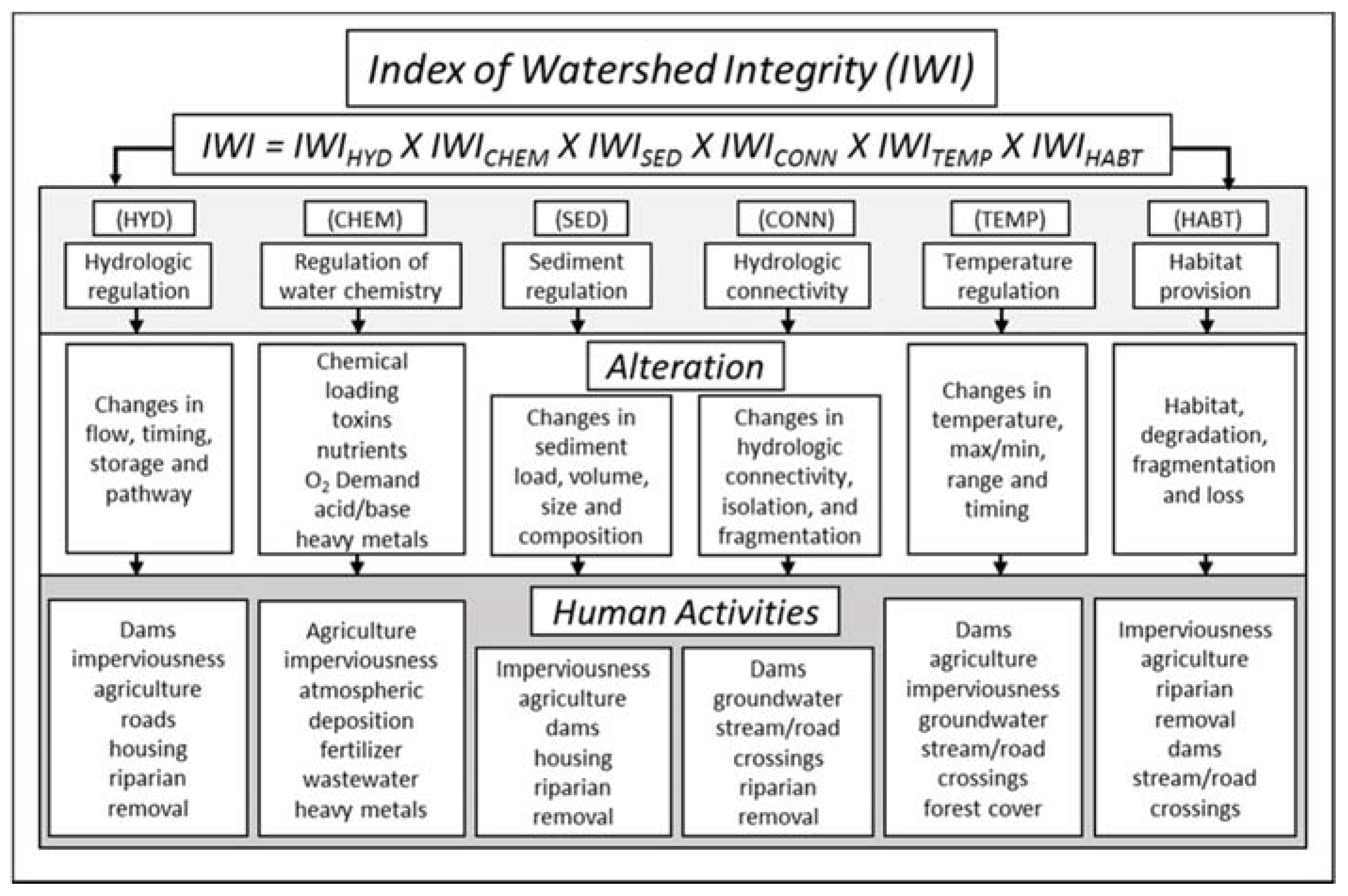
| Key Function | Description | Major Stressors | |
|---|---|---|---|
| Within Channel | Outside Channel | ||
| HYD | Maintenance of the natural timing, pattern, supply, and storage of water that flows through the watershed | Presence and volumes of reservoirs (NABD) Stream channelization and levee construction (NA) | Percent of the watershed comprising agricultural land use (NLCD) Total length and density of canals/ditches (NHD) Percent imperviousness of human-related landscapes (NLCD) Alteration to and spatial arrangement of riparian vegetation (LANDFIRE) Boundaries, depths, and flows of aquifers (NA) Groundwater use (NA) * |
| CHEM | Maintenance of the natural timing, supply, and storage of the major chemical constituents of freshwaters: nutrients (nitrogen and phosphorus), salinity or conductivity, total dissolved solids, hydrogen ions (pH), and naturally occurring minor constituents (e.g., heavy metals). Human-related alterations can include deviations from naturally occurring concentrations of these constituents or the inclusion of non-naturally occurring constituents, such as pesticides and industrial chemicals. | Presence and volumes of reservoirs (NABD) Stream channelization and levee construction (NA) | Atmospheric deposition of anthropogenic sources of nitrogen and acid rain (NADP) Percent of watershed composed of urban and agricultural land uses (NLCD) Fertilizer application rates (FERT) Presence and density of wastewater treatment facilities (NPDES), industrial facilities (TRI), superfund sites (SUPERFUND), and mines (MINES) Cattle density (NA) * Alteration to and spatial arrangement of riparian vegetation (LANDFIRE) Chemical constituents of groundwater (NA) |
| SED | Maintenance of the volume and size composition of inorganic particles that are stored or transported through the stream or within lakes, wetlands, or estuaries. | Presence and volumes of reservoirs (NABD) Stream channelization and levee construction (NA) | Alteration to and spatial arrangement of riparian vegetation (LANDFIRE) Presence and density of mines (MINES), forest cover loss (GFC), and roads (TIGER) Agriculture (NLCD) weighted by soil erodibility (CONUS-SOIL) |
| CONN | Presence of hydrologic pathways for the transfer of matter, energy, genes, and organisms within watersheds. Systems can vary naturally in their hydrologic isolation (e.g., desert springs) or connectedness (e.g., the Everglades). | Presence and volumes of reservoirs (NABD) Stream channelization and levee construction (NA) Road/stream intersections (TIGER/NHD) weighted by stream reach slope (NHD) | Alteration to and spatial arrangement of riparian vegetation (LANDFIRE) Density of ditches/canals (NHD) Groundwater use (NA) * Presence and density of wastewater discharge sites (NPDES) Percent of riparian zone composed of urban and agricultural land uses (NLCD) |
| TEMP | Maintenance of the full range of natural landscape features (both aquatic and terrestrial) required to maintain temperatures that support the aquatic chemistry and biota. | Presence and volumes of reservoirs (NABD) | Alteration to and spatial arrangement of riparian vegetation (LANDFIRE) Percent of watershed composed of agricultural land uses (NLCD) Percent of watershed composed of urban land uses in the riparian zone (NLCD) Groundwater use (NA) * Presence and density of wastewater discharge sites (NPDES) |
| HABT | Presence and maintenance of the full range of natural landscape features (both aquatic and terrestrial) that represent the complete set of conditions that are needed to maintain the natural diversity and abundances of aquatic biota. | Presence and volumes of reservoirs (NABD) | Alteration to and spatial arrangement of riparian vegetation (LANDFIRE) Density of housing unit developments within riparian zones (TIGER) Percent of watershed composed of agricultural land uses (NLCD) Density of road/stream intersections (TIGER/NHD) Density of roads within riparian zones (TIGER) |
| Variable | HYD | CHEM | SED | CONN | TEMP | HABT |
|---|---|---|---|---|---|---|
| PctUrb2006Ws | X | |||||
| PctAg2006Ws | X | X | X | X | ||
| PctImp2006Ws | X | |||||
| RdDensWs | X | |||||
| RdCrsWs | X | |||||
| NABD_DensWs | X | X | X | X | X | X |
| NABD_NrmStorWs | X | X | X | X | X | X |
| AgKffactWs | X | |||||
| MineDensWs | X | X | ||||
| CoalMineDensWs | X | X | ||||
| CanalDensWs | X | X | ||||
| RdCrsSlpWtdWs | X | |||||
| InorgNWetDepWs | X | |||||
| FertWs | X | |||||
| NPDESDensWs | X | X | X | |||
| TRIDensWs | X | |||||
| SuperfundDensWs | X | |||||
| PctUrb2006WsRp100 | X | X | ||||
| PctAg2006WsRp100 | X | |||||
| PctNonAgIntrodManagVegWsRp100 | X | X | X | X | X | X |
| PctFrstLoss2006Ws | X | |||||
| RdDensWsRp100 | X | |||||
| HUDens2010WsRp100 | X |
| Variable Name | Description |
|---|---|
| PctUrb2006Ws | % of watershed area classified as developed, high, medium, and low-intensity land use (NLCD 2006 class 22, 23, 24) |
| PctAg2006Ws | % of watershed area classified as crop and hay land use (NLCD 2006 class 81 and 82) |
| PctImp2006Ws | % imperviousness of anthropogenic surfaces within watershed |
| RdDensWs | Density of roads (2010 Census Tiger Lines) within watershed (km/km2) |
| RdCrsWs | Density of roads-stream intersections (2010 Census Tiger Lines-NHD stream lines) within watershed (crossings/km2) |
| NABD_DensWs | Density of georeferenced dams within watershed (dams/km2) |
| NABD_NrmStorWs | Volume all reservoirs (NORM_STORA in NID) per unit area of watershed (cubic meters/km2) |
| AgKffactWs | The Kffact is used in the Universal Soil Loss Equation (USLE) and represents a relative index of susceptibility of bare, cultivated soil to particle detachment and transport by rainfall within watershed |
| MineDensWs | Density of mines sites within watershed (mines/km2) |
| CoalMineDensWs | Density of coal mines within the watershed (mines/km2) |
| CanalDensWs | Density of NHDPlus line features classified as canal, ditch, or pipeline within the upstream watershed (km/km2) |
| RdCrsSlpWtdWs | Mean stream slope (NHD stream slope) of roads-stream intersections (2010 Census Tiger Lines-NHD stream lines) within watershed (crossings/km2) |
| InorgNWetDepWs | Annual gradient map of precipitation-weighted mean deposition for inorganic nitrogen wet deposition from nitrate and ammonium for 2008 in kg of NH4+ ha/year, within watershed |
| FertWs | Mean rate of synthetic nitrogen fertilizer application to agricultural land in kg N/ha/year, within watershed |
| NPDESDensWs | Density of permitted NPDES (National Pollutant Discharge Elimination System) sites within watershed (sites/km2) |
| TRIDensWs | Density of TRI (Toxic Release Inventory) sites within watershed (sites/km2) |
| SuperfundDensWs | Density of Superfund sites within watershed and within 100-m buffer of NHD stream lines (sites/km2) |
| PctUrb2006WsRp100 | % of watershed area classified as developed, high, medium, and low -intensity land use (NLCD 2006 class 22, 23, 24) within a 100-m buffer of NHD streams |
| PctAg2006WsRp100 | % of watershed area classified as crop and hay land use (NLCD 2006 class 81 and 82) within a 100-m buffer of NHD streams |
| PctFrstLoss2006Ws | % Forest cover loss (Tree canopy cover change) for 2006 within watershed |
| PctNonAgIntrodManag VegWsRp100 | % Non-agriculture non-native introduced or managed vegetation landcover type reclassed from LANDFIRE Existing Vegetation Type (EVT), within watershed and within 100-m buffer of NHD stream lines |
| RdDensWsRp100 | Density of roads (2010 Census Tiger Lines) within watershed and within 100-m buffer of NHD stream lines (km/km2) |
| HUDen2010WsRp100 | Mean housing unit density (housing units/km2) within watershed and within a 100-m buffer of NHD stream lines |
| Watershed | Calapooia River | Choptank Study Area | East Fork Little Miami River | Narragansett Bay |
|---|---|---|---|---|
| Size (km2) | 945 | 1070 | 1293 | 4421 |
| Elevation range (m) | 57–1562 | 0–36 | 149–365 | 0–423 |
| Land Use Classification a | ||||
| % Agriculture | 52.6 | 59.5 | 55 | 6.3 |
| % Forest | 28.7 | 11.7 | 32 | 38.9 |
| % Brushland | 11.8 | 1.2 | 0.27 | 0.98 |
| % Urban/Developed | 5.11 | 6.4 | 11.4 | 34.7 |
| % Wetland | 1.6 | 20.4 | 0.16 | 14.9 |
| % Open Water | 0.07 | 0.8 | 1.1 | 3.4 |
| % Impervious Surface | 1.82 | 0.85 | 2.51 | 14.96 |
| Population b (2010) | 28,959 | 37,164 | 129,670 | 1,962,003 |
| Population Density (Persons/km2) | 30 | 35 | 100 | 442 |
| Annual Average Precipitation c (cm) | 145 | 111 | 108 | 125 |
| River Kilometer (km) | 619 | 812 | 1251 | 2489 |
| Type | Response Variable | Response Variable Description | Sample Sites (n) |
|---|---|---|---|
| CRW | |||
| S | δ15N chironomid | Chironomid nitrogen isotopic composition (δ15N ‰) collected from 2013–2015 | 22 |
| S | log10Naavg | Log10 of the average NO3 concentrations of each month over the entire sampling period were calculated at each site. | 53 |
| S | log10Ndif | Ndif, calculated as the difference between the highest and lowest monthly values of log10 NO3 concentrations at each site. | 53 |
| S | TN_in (kg N/ha/year) | Annual total nitrogen (TN) input from all anthropogenic and natural sources. Indices were calculated in the Calapooia River Watershed N budget project [37] see Supplementary Materials. | 13 |
| S | TN_out (kg N/ha/year) | Annual total nitrogen (TN) export using LOADEST model (U.S. Geological Survey, Reston, VA, USA). Indices were calculated in the Calapooia River Watershed N budget project [37] see Supplementary Materials. | 13 |
| S | ag_frt (kg N/ha/year) | Annual TN input from fertilization. Indices were calculated in the Calapooia River Watershed N budget project [37] see Supplementary Materials. | 13 |
| S | winter_frt (kg N/ha) | Fertilizer N input in winter. Indices were calculated in the Calapooia River Watershed N budget project [37] see Supplementary Materials. | 13 |
| S | harvest (kg N/ha/year) | Annual N removal via crop harvest. Indices were calculated in the Calapooia River Watershed N budget project [37] see Supplementary Materials. | 13 |
| S | resN (kg N/ha/year) | Retention N—difference between annual TN input and annual TN export. Indices were calculated in the Calapooia River Watershed N budget project [37] see Supplementary Materials. | 13 |
| S | fishMMI | Fish MMIs were calculated following methods set by Whittier et al. [45]. Seven metrics for the Western Mountains Ecoregion were selected and consisted of an assemblage tolerance index estimating overall resilience to disturbance [45]. Scores were generated for each unique sampling event and a mean inter-annual score was attributed to sites receiving multiple visits over the course of the study. Final scores were rescaled to values between 0 and 100 for comparison with the IWI, with increasing scores indicating higher overall ecological condition. Sampling occurred throughout the year but for consistency only NRSA index period data were used for this analysis (summer low-flow conditions). | 36 |
| S | max_tempC_summer | Maximum summer temperature metric derived from a database containing seven years (2009–2015) of 30-min time series temperature logger data from 87 established sites the Calapooia basin. Maximum summer temperature was defined as the absolute maximum observation during the warmest period of the year in western Oregon, July–August. The maximum temperature value across all years considered was assigned to each site as a final representative maximum summer temperature metric. | 36 |
| S | amplitude | Amplitude and phase metrics for stream temperatures were calculated following the methods of Maheu et al. [42] to fit a sine curve to continuous time series data for each sample site and examine the magnitude and timing of temperature change throughout the year. This method provides a generalizable index of thermal regime magnitude (amplitude). | 64 |
| S | phase | Amplitude and phase metrics for stream temperatures were calculated following the methods of Maheu et al. [42] to fit a sine curve to continuous time series data for each sample site and examine the magnitude and timing of temperature change throughout the year. This method provides a generalizable index of thermal regime timing (phase). | 64 |
| S | v1w_msq | Large wood volumetric density (m3/m2), a measure of channel complexity and roughness. The physical habitat of stream segments was characterized using the methods of Kaufmann [39]. Data were collected 2013–2015 during the summer low-flow season. | 19 |
| S | sedembed | Sediment embeddedness (%), a measure of the degree to which substrate cobbles and gravels are encompassed by finer sediments. The physical habitat of stream segments was characterized using the methods of Kaufmann [39]. Data were collected 2013–2015 during the summer low-flow season. | 20 |
| S | sddepth | Morphology, using an index of variation in longitudinal variation in channel depth; a measure of pool/riffle ratio. The physical habitat of stream segments was characterized using the methods of Kaufmann [39]. Data were collected 2013–2015 during the summer low-flow season. | 20 |
| S | xfc_nat | In-channel cover (%), an index of channel complexity relevant to fish. The physical habitat of stream segments was characterized using the methods of Kaufmann [39]. Data were collected 2013–2015 during the summer low-flow season. | 20 |
| S | vegcovrip | Riparian vegetation cover (%), an index of riparian vegetation density and complexity. The physical habitat of stream segments was characterized using the methods of Kaufmann [39]. Data were collected 2013–2015 during the summer low-flow season. | 20 |
| CHOP | |||
| W | wetareasqm | Area of wetland polygons intersecting stream channels in a catchment in sq meters calculated using GIS tool ‘Tabulate by Intersection’ using NWI V2 and NHD v2 (and LiDAR) stream networks to quantify stream-wetland connectivity metrics. | 523 |
| W | wetpercentage | Percentage of areal coverage for wetland polygons intersecting stream channels in a catchment using GIS tool ‘Tabulate by Intersection’ using NWI V2 and NHD v2 (and LiDAR) stream networks to quantify stream-wetland connectivity metrics. | 523 |
| W | wetcntwhole | Count of whole wetland polygons in catchment calculated using GIS ‘Summarize FEATUREID on Spatial Join’ using NWI V2 and NHD v2 (and LiDAR) stream networks to quantify stream-wetland connectivity metrics. | 523 |
| W | wetcntpartial | Count of partial wetland polygons in catchment calculated using GIS ‘Summarize FEATUREID on Intersect’ using NWI V2 and NHD v2 (and LiDAR) stream networks to quantify stream-wetland connectivity metrics. | 523 |
| W | wetcntall | Count of total wetland polygons calculated as: Sum of wetcntwhole + wetcntpartial using NWI V2 and NHD v2 (and LiDAR) stream networks to quantify stream-wetland connectivity metrics. | 523 |
| EFLMR | |||
| S | log10Tavg | Log10 of the annual Total-N: Data collected between 2005 and 2015; Multiple site-analysis measurements within a day were averaged. Total Inorganic-N values greater than Total N values were removed from the analysis. Data were then organized by month between 2005–2015 and monthly average values were calculated for each site-analysis pairing. | 43 |
| S | log10TNH4aavg | Log10 of the annual total ammonium: Data collected between 2005 and 2015; Multiple site-analysis measurements within a day were averaged. Data were then organized by month between 2005–2015 and monthly average values were calculated for each site-analysis pairing. | 43 |
| S | log10TNOxaavg | Log10 of the annual total nitrate/nitrite: Data collected between 2005 and 2015; Multiple site-analysis measurements within a day were averaged. Data were then organized by month between 2005–2015 and monthly average values were calculated for each site-analysis pairing. | 44 |
| S | log10INavg | Data collected between 2005 and 2015; Multiple site-analysis measurements within a day were averaged. Data were then organized by month between 2005–2015 and monthly log10 of the average values were calculated for each site-analysis pairing. | 44 |
| S | log10fINavg | Fraction of Total-N as Inorganic-N: Data collected between 2005 and 2015; Multiple site-analysis measurements within a day were averaged. Data were then organized by month between 2005–2015 and monthly log10 of the average values were calculated for each site-analysis pairing. | 38 |
| S | log10TNdif | Annual range in Total-N: Monthly average values were used to compute the annual concentration fluctuation—Ndif, calculated as the difference between the highest and lowest monthly values of log10 Total-N concentrations. | 43 |
| S | log10TNH4dif | Annual range in total ammonium: Monthly average values were used to compute the annual concentration fluctuation—NH4dif, calculated as the difference between the highest and lowest monthly values of log10 total-ammonium concentrations. | 43 |
| S | log10TNOxdif | Annual range in total nitrate/nitrite: Monthly average values were used to compute the annual concentration fluctuation—NOxdif, calculated as the difference between the highest and lowest monthly values of log10 total nitrate/nitrite concentrations. | 44 |
| S | log10INdif | Annual range in Inorganic-N: Monthly average values were used to compute the annual concentration fluctuation—INdif, calculated as the difference between the highest and lowest monthly values of log10 Inorganic-N concentrations. | 44 |
| S | log10fINdif | Annual range in fraction of Total-N as Inorganic-N: Monthly average values were used to compute the annual concentration fluctuation—fINdif, calculated as the difference between the highest and lowest monthly values of fraction of log10 Total-N as Inorganic-N concentrations. | 38 |
| NBW | |||
| S | δ15N periphyton | Nitrogen isotopic composition (δ15N ‰) of periphyton collected from six randomly selected rocks (composite sample) at stream sites within Narragansett Bay Watershed in 2012 | 69 |
| S | log10tn | Total nitrogen log 10 transformed-water sample collected from stream sites in 2012 | 71 |
| S | log10no3 | NO3 concentration log 10 transformed-water sample collected from stream sites in 2012 | 71 |
| S | log10nh4 | NH4 concentration log 10 transformed-water sample collected from stream sites in 2012 | 71 |
| S | log10chloride | Chloride concentration log 10 transformed- water sample collected from stream sites in 2012 | 71 |
| L | δ15N BOM | Nitrogen isotopic composition (δ15N ‰) of benthic organic matter (BOM) collected from surficial sediments in littoral zone of lakes | 51 |
| Case Study Watershed | Index of Watershed Integrity | Index of Catchment Integrity | ||||||||||||
|---|---|---|---|---|---|---|---|---|---|---|---|---|---|---|
| min | 25% | mean | median | 75% | max | SD | min | 25% | mean | median | 75% | max | SD | |
| CRW | 0.418 | 0.642 | 0.789 | 0.876 | 0.962 | 0.982 | 0.195 | 0.423 | 0.495 | 0.732 | 0.75 | 0.959 | 0.983 | 0.225 |
| CHOP | 0.403 | 0.511 | 0.556 | 0.55 | 0.594 | 0.822 | 0.069 | 0.386 | 0.509 | 0.601 | 0.578 | 0.662 | 0.957 | 0.128 |
| EFLMR | 0.409 | 0.456 | 0.546 | 0.494 | 0.638 | 0.918 | 0.117 | 0.403 | 0.513 | 0.62 | 0.592 | 0.754 | 0.923 | 0.138 |
| NBW | 0.427 | 0.674 | 0.746 | 0.764 | 0.837 | 0.923 | 0.113 | 0.418 | 0.675 | 0.75 | 0.754 | 0.865 | 0.925 | 0.122 |
| Watersheds Combined Sampled Sites | 0.403 | 0.52 | 0.641 | 0.588 | 0.747 | 0.982 | 0.162 | 0.386 | 0.518 | 0.659 | 0.614 | 0.793 | 0.983 | 0.171 |
| Watersheds Combined All Sites a | 0.19 | 0.562 | 0.68 | 0.691 | 0.796 | 1 | 0.146 | 0.125 | 0.571 | 0.7 | 0.71 | 0.831 | 1 | 0.157 |
| Index | Vegcovrip | TN_in | Sedembed | Phase | Max_tempC_Summer | log10Ndif | log10NAavg | Fish MMI | δ15N Chironomid |
|---|---|---|---|---|---|---|---|---|---|
| IWI | 0.65 | −0.97 | −0.77 | 0.77 | −0.73 | −0.93 | −0.92 | 0.82 | −0.92 |
| ICI | 0.52 | −0.96 | −0.75 | 0.76 | −0.91 | −0.82 | −0.77 | 0.83 | −0.89 |
| WCHEM | 0.63 | −0.99 | −0.74 | 0.77 | −0.70 | −0.91 | −0.91 | 0.79 | −0.88 |
| CCHEM | 0.49 | −0.98 | −0.74 | 0.74 | −0.89 | −0.84 | −0.79 | 0.81 | −0.87 |
| WHABT | 0.59 | −0.97 | −0.71 | 0.75 | −0.68 | −0.90 | −0.90 | 0.78 | −0.87 |
| CHABT | 0.48 | −0.97 | −0.72 | 0.75 | −0.88 | −0.82 | −0.76 | 0.80 | −0.86 |
| WSED | 0.57 | −0.98 | −0.69 | 0.75 | −0.67 | −0.89 | −0.91 | 0.73 | −0.82 |
| CSED | 0.45 | −0.98 | −0.68 | 0.76 | −0.87 | −0.84 | −0.80 | 0.77 | −0.83 |
| WHYD | 0.63 | −0.99 | −0.74 | 0.77 | −0.71 | −0.90 | −0.90 | 0.78 | −0.88 |
| CHYD | 0.49 | −0.98 | −0.75 | 0.73 | −0.87 | −0.83 | −0.78 | 0.80 | −0.86 |
| WTEMP | 0.63 | −0.98 | −0.74 | 0.77 | −0.71 | −0.90 | −0.90 | 0.79 | −0.88 |
| CTEMP | 0.48 | −0.98 | −0.73 | 0.75 | −0.90 | −0.82 | −0.76 | 0.81 | −0.86 |
| WCONN | 0.72 | −0.94 | −0.82 | 0.71 | −0.65 | −0.92 | −0.91 | 0.84 | −0.93 |
| CCONN | 0.58 | −0.92 | −0.78 | 0.74 | −0.87 | −0.70 | −0.66 | 0.83 | −0.87 |
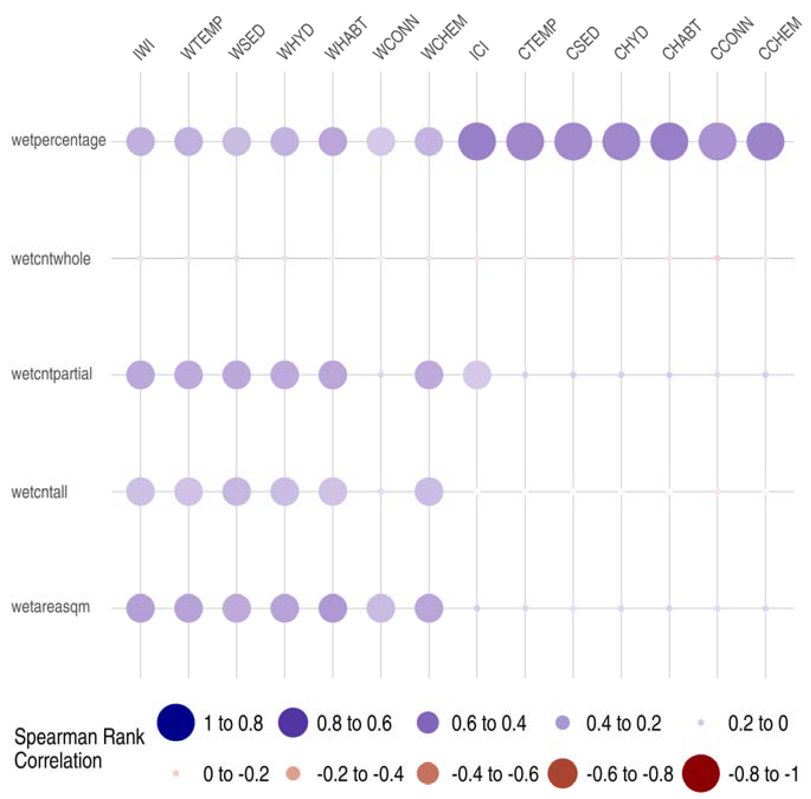
| Index | Wetareasqm | Wetpercentage | Wetcntall | Wetcntwhole | Wetcntpartial |
|---|---|---|---|---|---|
| IWI | 0.36 *** | 0.30 *** | 0.24 *** | 0.10 * | 0.33 *** |
| ICI | 0.19 *** | 0.49 *** | 0.01 - | −0.11 ** | 0.20 *** |
| WHYD | 0.35 *** | 0.29 *** | 0.25 *** | 0.11 * | 0.32 *** |
| CHYD | 0.16 ** | 0.46 *** | 0.03- | −0.07- | 0.19 *** |
| WCHEM | 0.34 *** | 0.28 *** | 0.25 *** | 0.10 * | 0.32 *** |
| CCHEM | 0.16 ** | 0.47 *** | 0.02- | −0.09- | 0.19 *** |
| WSED | 0.32 *** | 0.26 *** | 0.27 *** | 0.13 ** | 0.33 *** |
| CSED | 0.13 ** | 0.45 *** | 0.01- | −0.12 * | 0.19 *** |
| WCONN | 0.26 *** | 0.21 *** | 0.13 ** | 0.06- | 0.16 ** |
| CCONN | 0.14 ** | 0.41 *** | −0.10 * | −0.19 *** | 0.14 ** |
| WTEMP | 0.35 *** | 0.30 *** | 0.23 *** | 0.09- | 0.32 *** |
| CTEMP | 0.16 ** | 0.46 *** | 0.01- | −0.09- | 0.18 *** |
| WHABT | 0.39 *** | 0.34 *** | 0.23 *** | 0.07- | 0.34 *** |
| CHABT | 0.18 *** | 0.49 *** | 0.01- | −0.11 * | 0.19 *** |
| Index | log10T avg | log10TNH4aavg | log10TNOxaavg | log10INavg | log10fINavg | log10TNdif | log10TNH4dif | log10TNOxdif | log10INdif | log10fINdif |
|---|---|---|---|---|---|---|---|---|---|---|
| IWI | −0.78 *** | −0.44 *** | −0.64 *** | −0.64 *** | 0.01 | −0.61 *** | −0.27 *** | −0.76 *** | −0.65 *** | −0.1 |
| ICI | −0.56 *** | −0.51 *** | −0.46 *** | −0.5 *** | 0.05 | −0.54 *** | −0.45 *** | −0.61 *** | −0.58 *** | −0.34 *** |
| WCHEM | −0.72 *** | −0.4 *** | −0.63 *** | −0.62 *** | −0.03 | −0.56 *** | −0.25 *** | −0.74 *** | −0.62 *** | −0.11 ** |
| CCHEM | −0.53 *** | −0.46 *** | −0.49 *** | −0.52 *** | −0.03 | −0.51 *** | −0.4 *** | −0.6 *** | −0.56 *** | −0.33 *** |
| WHABT | −0.8 *** | −0.48 *** | −0.65 *** | −0.66 *** | 0.01 | −0.64 *** | −0.3 *** | −0.77 *** | −0.67 *** | −0.13 ** |
| CHABT | −0.56 *** | −0.49 *** | −0.46 *** | −0.5 *** | 0.06 | −0.56 *** | −0.43 *** | −0.62 *** | −0.6 *** | −0.39 *** |
| WSED | −0.8 *** | −0.49 *** | −0.59 *** | −0.61 *** | 0.08 | −0.68 *** | −0.33 *** | −0.77 *** | −0.69 *** | −0.13 ** |
| CSED | −0.62 *** | −0.52 *** | −0.48 *** | −0.53 *** | 0.09 | −0.66 *** | −0.45 *** | −0.68 *** | −0.67 *** | −0.44 *** |
| WHYD | −0.8 *** | −0.47 *** | −0.59 *** | −0.62 *** | 0.11 | −0.69 *** | −0.31 *** | −0.77 *** | −0.72 *** | −0.14 ** |
| CHYD | −0.57 *** | −0.48 *** | −0.44 *** | −0.49 *** | 0.16 | −0.64 *** | −0.44 *** | −0.65 *** | −0.65 *** | −0.43 *** |
| WTEMP | −0.78 *** | −0.45 *** | −0.63 *** | −0.64 *** | 0.03 | −0.61 *** | −0.28 *** | −0.74 *** | −0.65 *** | −0.1 ** |
| CTEMP | −0.51 *** | −0.52 *** | −0.41 *** | −0.46 *** | 0.06 | −0.5 *** | −0.48 *** | −0.55 *** | −0.55 *** | −0.31 *** |
| WCONN | −0.77 *** | −0.52 *** | −0.6 *** | −0.64 *** | 0.02 | −0.65 *** | −0.36 *** | −0.74 *** | −0.69 *** | −0.13 ** |
| CCONN | −0.45 *** | −0.52 *** | −0.32 *** | −0.39 *** | 0.05 | −0.37 *** | −0.47 *** | −0.41 *** | −0.44 *** | −0.06 − |
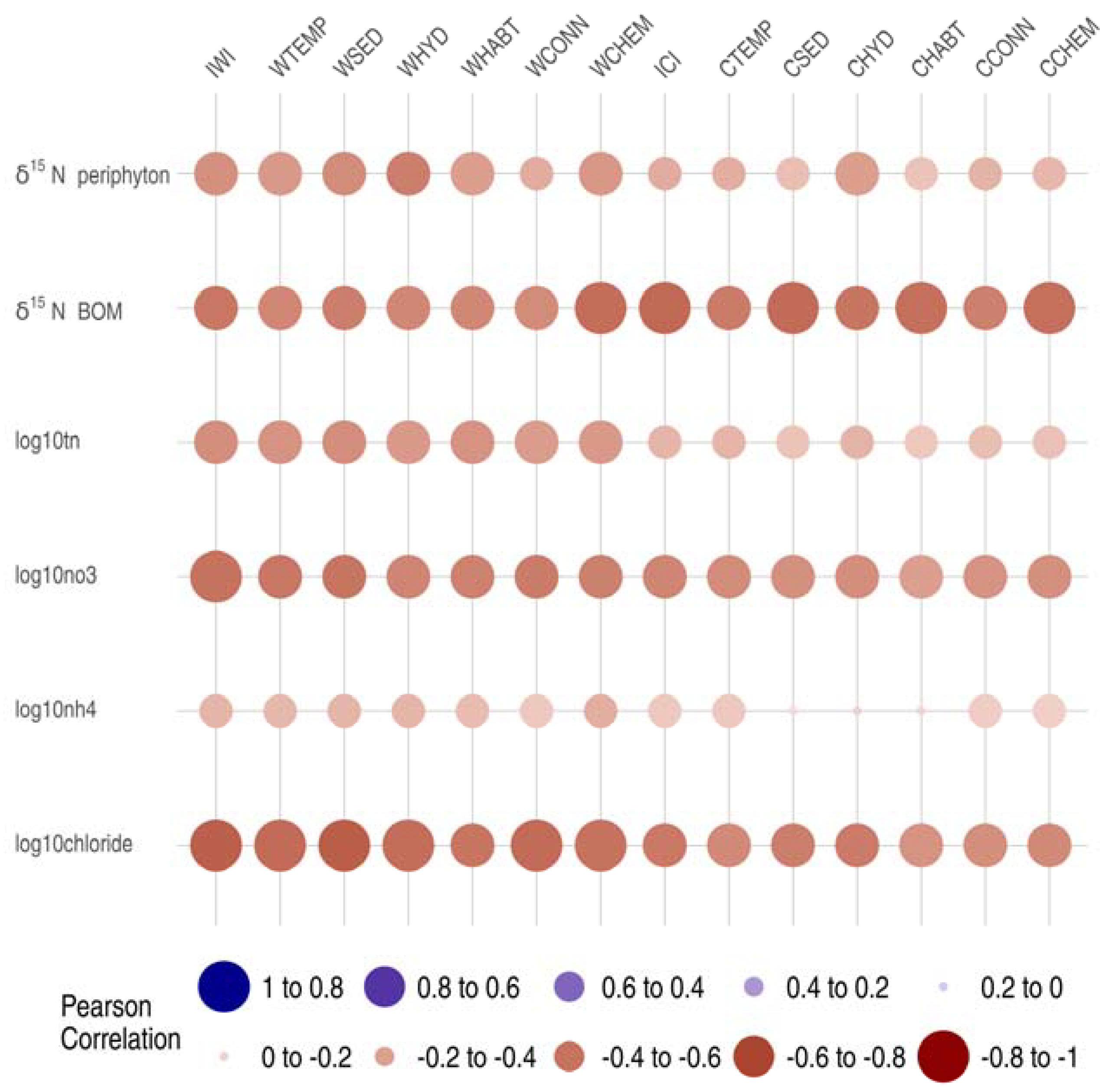
| Index | δ15N Periphyton | Log10tn | Log10no3 | Log10nh4 | Log10chloride | δ15N BOM |
|---|---|---|---|---|---|---|
| IWI | −0.47 *** | −0.48 *** | −0.6 *** | −0.31 *** | −0.68 *** | −0.58 *** |
| ICI | −0.35 *** | −0.31 *** | −0.52 *** | −0.23 *** | −0.57 *** | −0.64 *** |
| WCHEM | −0.44 *** | −0.43 *** | −0.54 *** | −0.34 *** | −0.6 *** | −0.62 *** |
| CCHEM | −0.3 *** | −0.26 *** | −0.47 *** | −0.2 *** | −0.5 *** | −0.61 *** |
| WHABT | −0.41 *** | −0.46 *** | −0.53 *** | −0.28 *** | −0.59 *** | −0.51 *** |
| CHABT | −0.25 *** | −0.23 *** | −0.41 *** | −0.18 *** | −0.46 *** | −0.61 *** |
| WSED | −0.49 *** | −0.48 *** | −0.59 *** | −0.31 *** | −0.69 *** | −0.55 *** |
| CSED | −0.27 *** | −0.25 *** | −0.47 *** | −0.15 ** | −0.55 *** | −0.63 *** |
| WHYD | −0.55 *** | −0.43 *** | −0.52 *** | −0.31 *** | −0.62 *** | −0.51 *** |
| CHYD | −0.41 *** | −0.32 *** | −0.48 *** | −0.19 *** | −0.56 *** | −0.59 *** |
| WTEMP | −0.43 *** | −0.46 *** | −0.58 *** | −0.3 *** | −0.63 *** | −0.51 *** |
| CTEMP | −0.34 *** | −0.31 *** | −0.49 *** | −0.23 *** | −0.5 *** | −0.56 *** |
| WCONN | −0.35 *** | −0.42 *** | −0.56 *** | −0.23 *** | −0.63 *** | −0.49 *** |
| CCONN | −0.32 *** | −0.27 *** | −0.46 *** | −0.21 *** | −0.48 *** | −0.54 *** |
| Response Variable | WATERSHED SCALE | CATCHMENT SCALE | ||||||||||||
|---|---|---|---|---|---|---|---|---|---|---|---|---|---|---|
| % Urb | % For | % Agr | IWI | % Max | Rank | # Exceed | % Urb | % For | % Agr | ICI | % Max | Rank | #Exceed | |
| CRW | ||||||||||||||
| δ15N chironomid | 0.45 | −0.79 | 0.83 | −0.92 | 100.0 | 1 | 3 | 0.12 | −0.86 | 0.83 | −0.89 | 100.0 | 1 | 3 |
| total_in | 0.92 | −0.87 | 0.98 | −0.97 | 99.0 | 2 | 2 | 0.85 | −0.86 | 0.98 | −0.96 | 98.0 | 2 | 2 |
| log10Ndif | 0.59 | −0.9 | 0.9 | −0.93 | 100.0 | 1 | 3 | 0.3 | −0.78 | 0.8 | −0.82 | 100.0 | 1 | 3 |
| EFLMR | ||||||||||||||
| log10Tavg | −0.56 | −0.72 | 0.8 | −0.78 | 97.5 | 2 | 2 | 0 | −0.57 | 0.54 | −0.56 | 98.2 | 2 | 2 |
| log10TNH4aavg | −0.39 | −0.39 | 0.49 | −0.44 | 89.8 | 2 | 2 | −0.07 | −0.43 | 0.47 | −0.51 | 100.0 | 1 | 3 |
| log10TNOxaavg | −0.28 | −0.63 | 0.57 | −0.64 | 100.0 | 1 | 3 | 0.14 | −0.53 | 0.4 | −0.46 | 86.8 | 2 | 2 |
| log10DIavg | −0.37 | −0.61 | 0.61 | −0.64 | 100.0 | 1 | 3 | 0.12 | −0.55 | 0.44 | −0.5 | 90.9 | 2 | 2 |
| log10fDIavg | 0.3 | −0.06 | −0.17 | 0.01 | 3.3 | 4 | 0 | 0.43 | −0.06 | −0.22 | 0.05 | 11.6 | 4 | 0 |
| log10TNdif | −0.61 | −0.53 | 0.72 | −0.61 | 84.7 | 2.5 | 1 | −0.29 | −0.49 | 0.65 | −0.54 | 83.1 | 2 | 2 |
| log10TNH4dif | −0.31 | −0.24 | 0.35 | −0.27 | 77.1 | 3 | 1 | −0.18 | −0.34 | 0.45 | −0.45 | 100.0 | 1.5 | 2 |
| log10TNOxdif | −0.49 | −0.72 | 0.76 | −0.76 | 100.0 | 1.5 | 2 | −0.1 | −0.62 | 0.63 | −0.61 | 96.8 | 3 | 1 |
| log10DINdif | −0.59 | −0.59 | 0.74 | −0.65 | 87.8 | 2 | 2 | −0.18 | −0.56 | 0.64 | −0.58 | 90.6 | 2 | 2 |
| log10fDINdif | −0.15 | −0.11 | 0.16 | −0.1 | 62.5 | 4 | 0 | −0.28 | −0.26 | 0.45 | −0.34 | 75.6 | 2 | 2 |
| NBW | ||||||||||||||
| δ15N periphyton | 0.45 | −0.5 | 0.11 | −0.47 | 94.0 | 2 | 2 | 0.39 | −0.48 | 0.07 | −0.35 | 72.9 | 3 | 1 |
| log10tn | 0.49 | −0.52 | −0.02 | −0.48 | 92.3 | 3 | 1 | 0.33 | −0.43 | 0.02 | −0.31 | 72.1 | 3 | 1 |
| log10NO3 | 0.55 | −0.47 | −0.07 | −0.6 | 100.0 | 1 | 3 | 0.52 | −0.51 | −0.07 | −0.52 | 100.0 | 1.5 | 2 |
| log10NH4 | 0.27 | −0.37 | −0.08 | −0.31 | 83.8 | 2 | 2 | 0.22 | −0.33 | −0.09 | −0.23 | 69.7 | 2 | 2 |
| log10chloride | 0.59 | −0.63 | −0.04 | −0.68 | 100.0 | 1 | 3 | 0.56 | −0.62 | −0.02 | −0.57 | 91.9 | 2 | 2 |
| δ15N BOM | 0.66 | −0.68 | 0.14 | −0.58 | 85.3 | 3 | 1 | 0.64 | −0.68 | 0.13 | −0.64 | 94.1 | 2.5 | 1 |
| CHOP | ||||||||||||||
| wetpercentage | −0.08 | 0.23 | −0.29 | 0.3 | 100.0 | 1 | 3 | −0.18 | 0.22 | −0.46 | 0.49 | 100.0 | 1 | 3 |
| wetcntall | −0.08 | 0.21 | −0.24 | 0.24 | 100.0 | 1.5 | 2 | 0.3 | 0.35 | −0.04 | 0.01 | 2.9 | 4 | 0 |
| wetcntwhole | −0.02 | 0.07 | −0.1 | 0.1 | 100.0 | 1.5 | 2 | 0.37 | 0.27 | 0.07 | −0.11 | 29.7 | 3 | 1 |
| wetcntpartial | −0.11 | 0.29 | −0.31 | 0.33 | 100.0 | 1 | 3 | 0.06 | 0.29 | −0.19 | 0.2 | 69.0 | 2 | 2 |
© 2018 by the authors. Licensee MDPI, Basel, Switzerland. This article is an open access article distributed under the terms and conditions of the Creative Commons Attribution (CC BY) license (http://creativecommons.org/licenses/by/4.0/).
Share and Cite
Kuhn, A.; Leibowitz, S.G.; Johnson, Z.C.; Lin, J.; Massie, J.A.; Hollister, J.W.; Ebersole, J.L.; Lake, J.L.; Serbst, J.R.; James, J.; et al. Performance of National Maps of Watershed Integrity at Watershed Scales. Water 2018, 10, 604. https://doi.org/10.3390/w10050604
Kuhn A, Leibowitz SG, Johnson ZC, Lin J, Massie JA, Hollister JW, Ebersole JL, Lake JL, Serbst JR, James J, et al. Performance of National Maps of Watershed Integrity at Watershed Scales. Water. 2018; 10(5):604. https://doi.org/10.3390/w10050604
Chicago/Turabian StyleKuhn, Anne, Scott G. Leibowitz, Zachary C. Johnson, Jiajia Lin, Jordan A. Massie, Jeffrey W. Hollister, Joseph L. Ebersole, James L. Lake, Jonathan R. Serbst, Jennifer James, and et al. 2018. "Performance of National Maps of Watershed Integrity at Watershed Scales" Water 10, no. 5: 604. https://doi.org/10.3390/w10050604
APA StyleKuhn, A., Leibowitz, S. G., Johnson, Z. C., Lin, J., Massie, J. A., Hollister, J. W., Ebersole, J. L., Lake, J. L., Serbst, J. R., James, J., Bennett, M. G., Brooks, J. R., Nietch, C. T., Smucker, N. J., Flotemersch, J. E., Alexander, L. C., & Compton, J. E. (2018). Performance of National Maps of Watershed Integrity at Watershed Scales. Water, 10(5), 604. https://doi.org/10.3390/w10050604