Modeling Hydroclimatic Change in Southwest Louisiana Rivers

 ,
,
Abstract
1. Introduction
2. Method
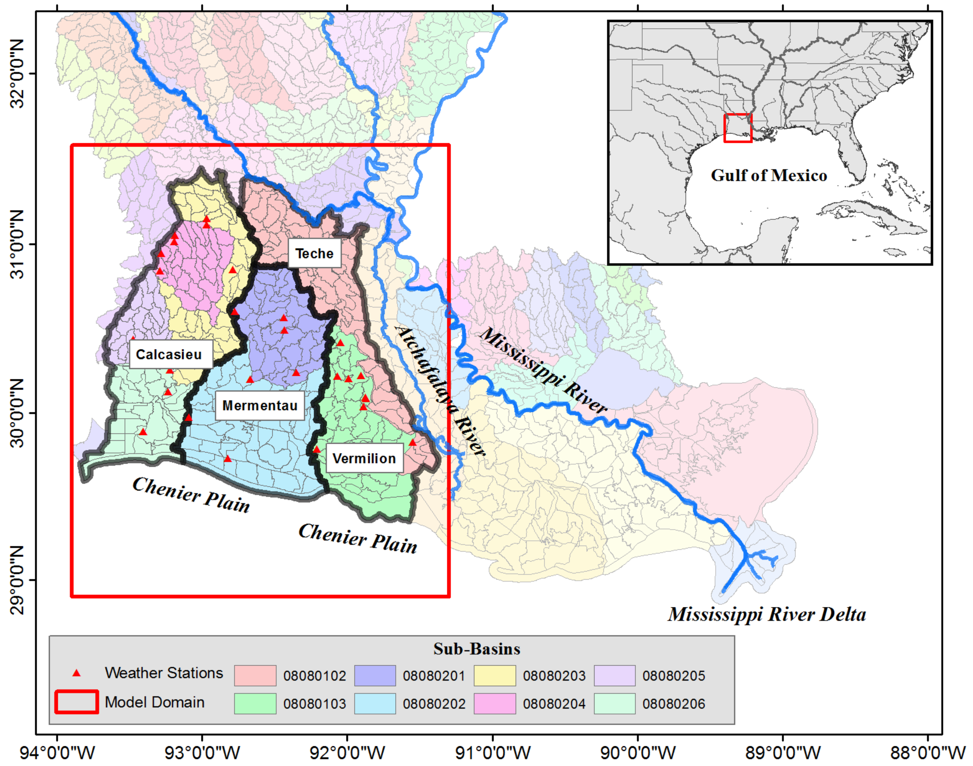
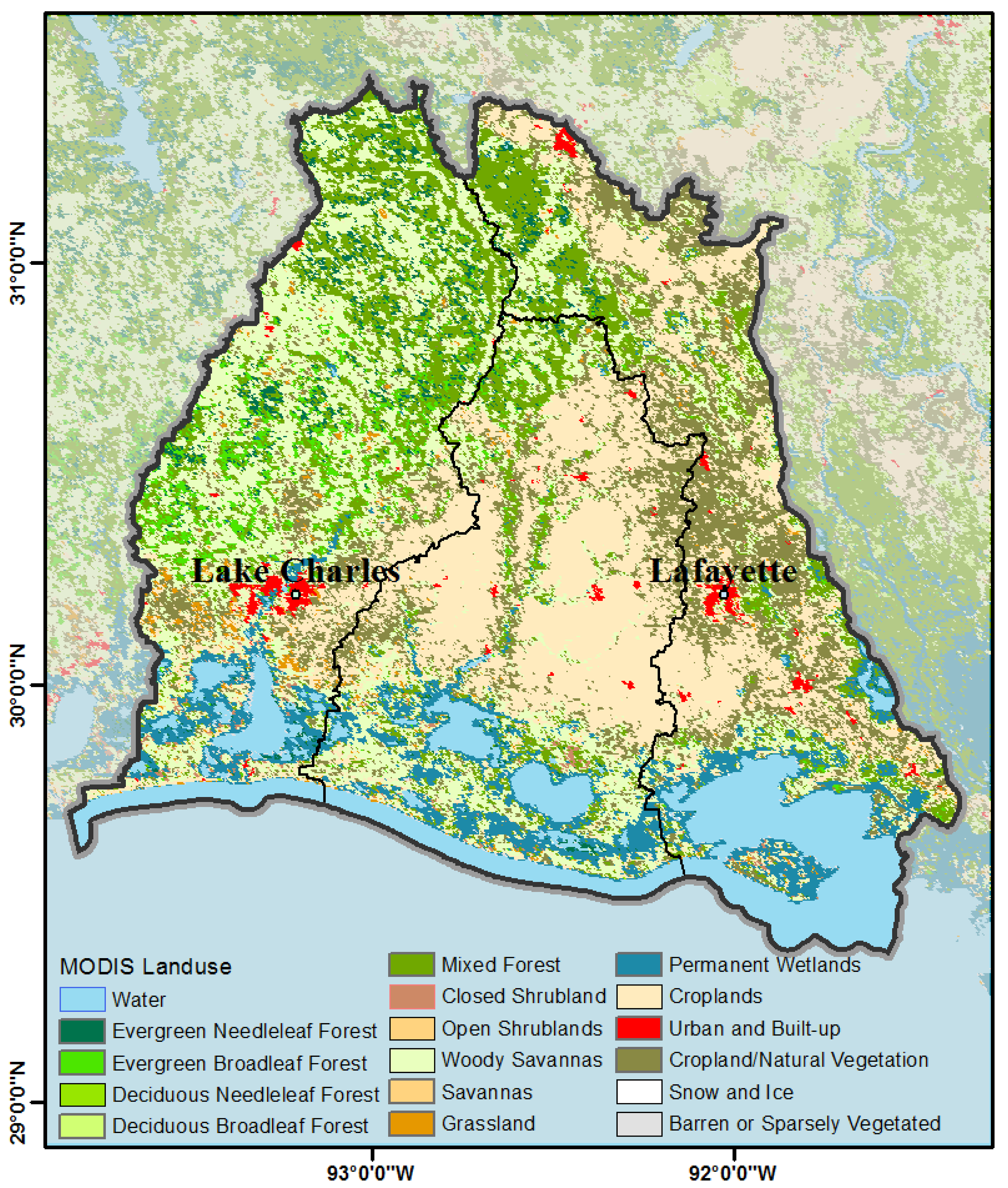
2.1. Study Area
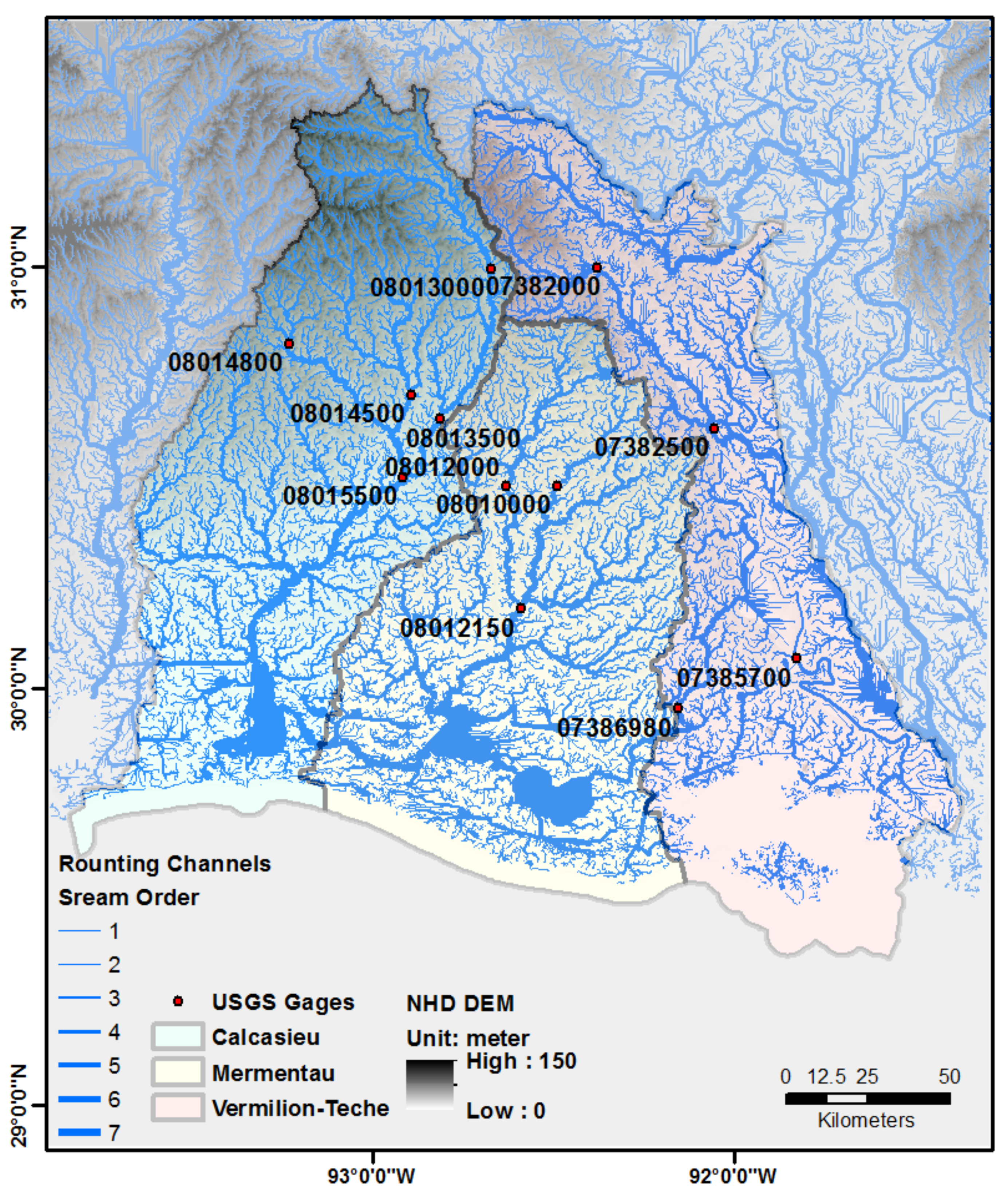
2.2. Model Setup
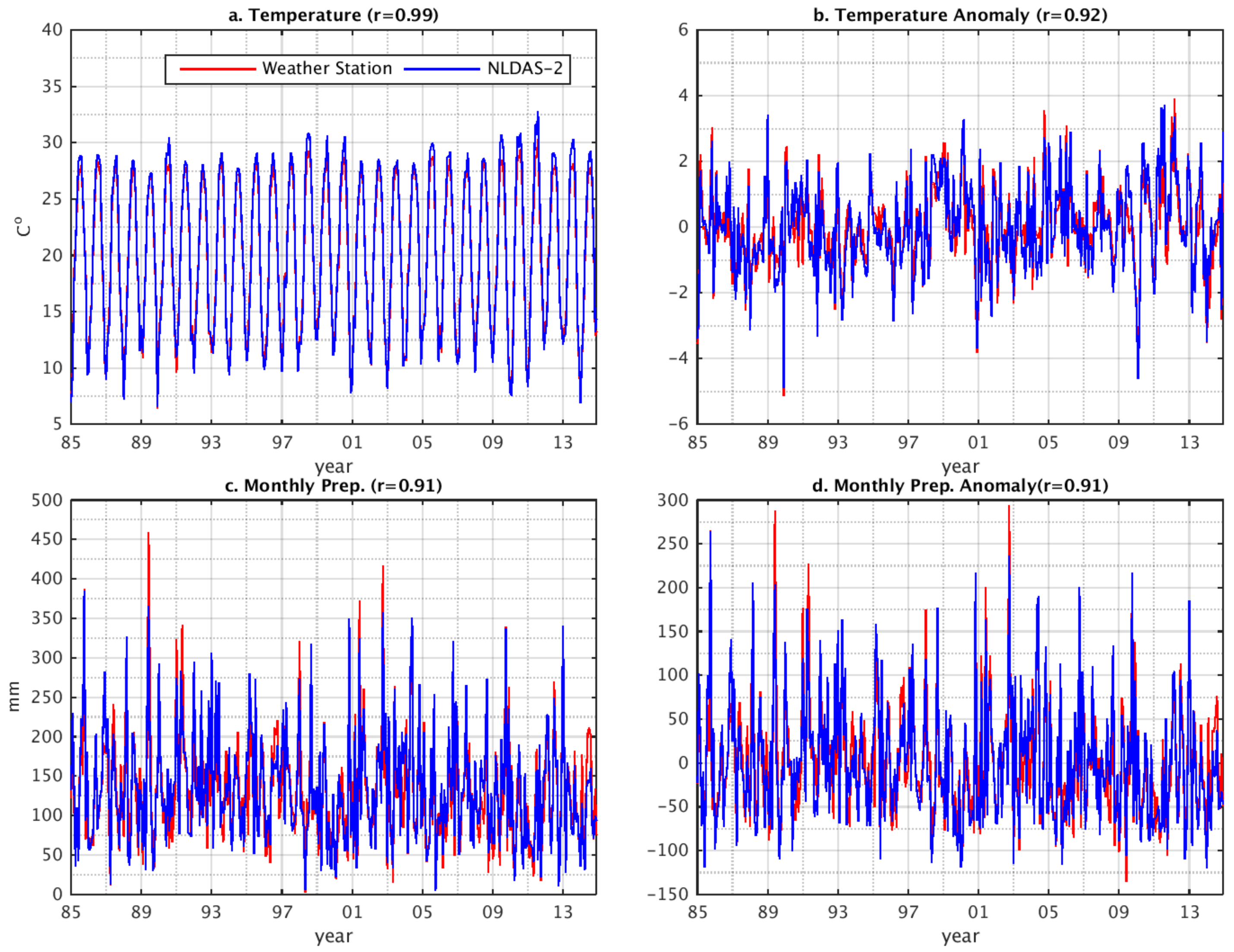
2.3. Evaluation of NLDAS-2 Data and WRF-Hydro
2.4. Trend and Wavelet Analysis
3. Results
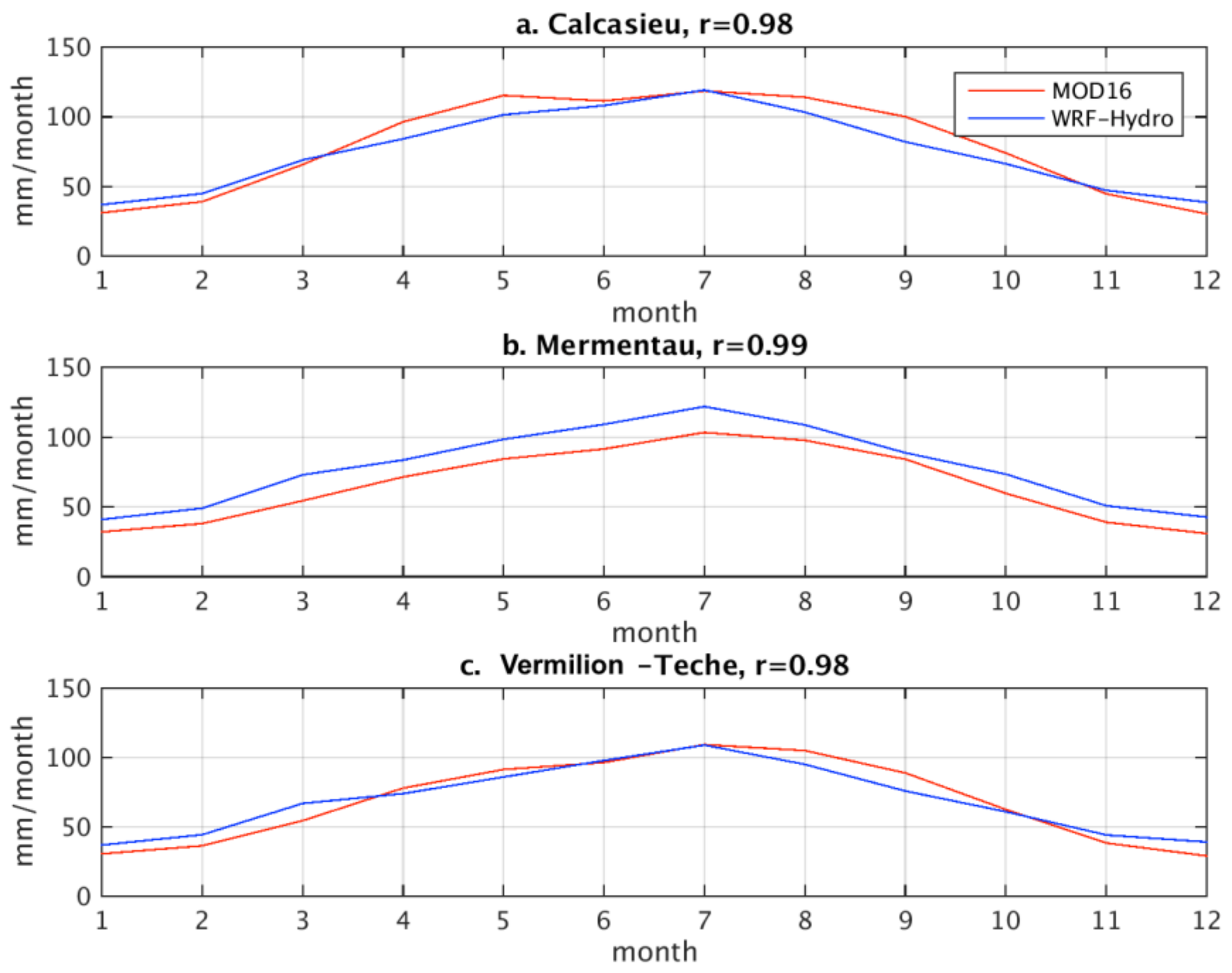
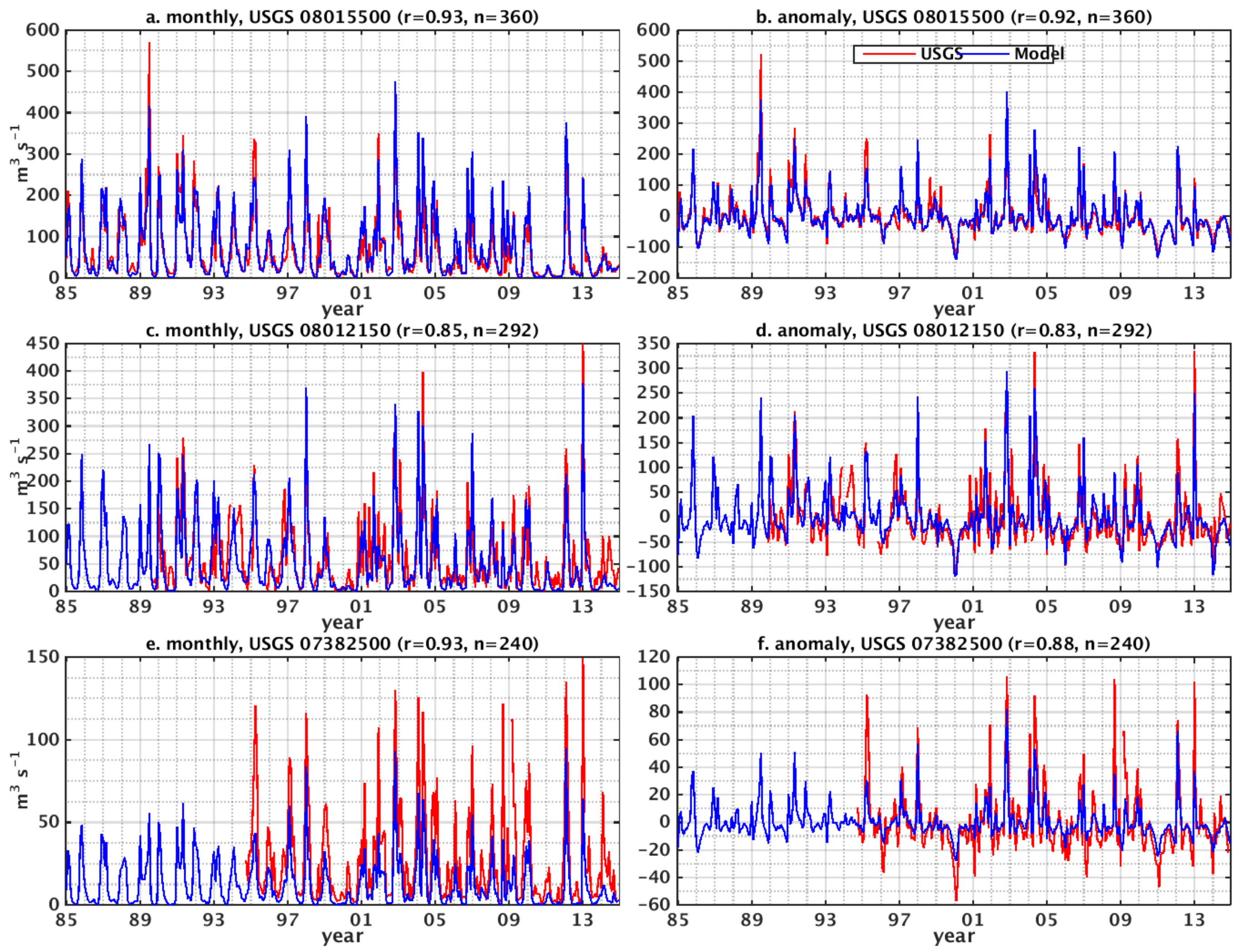
3.1. Model-Data Comparison
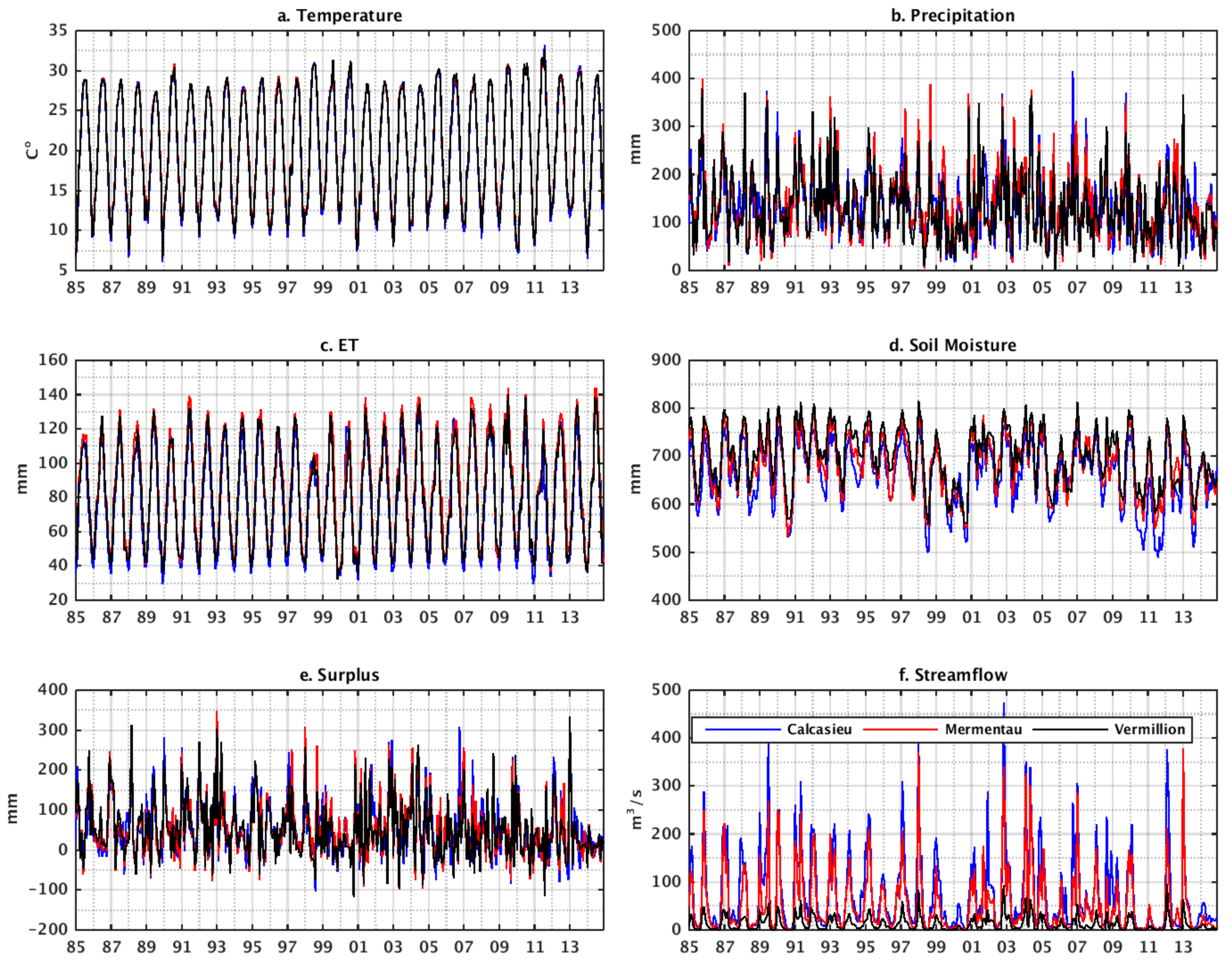
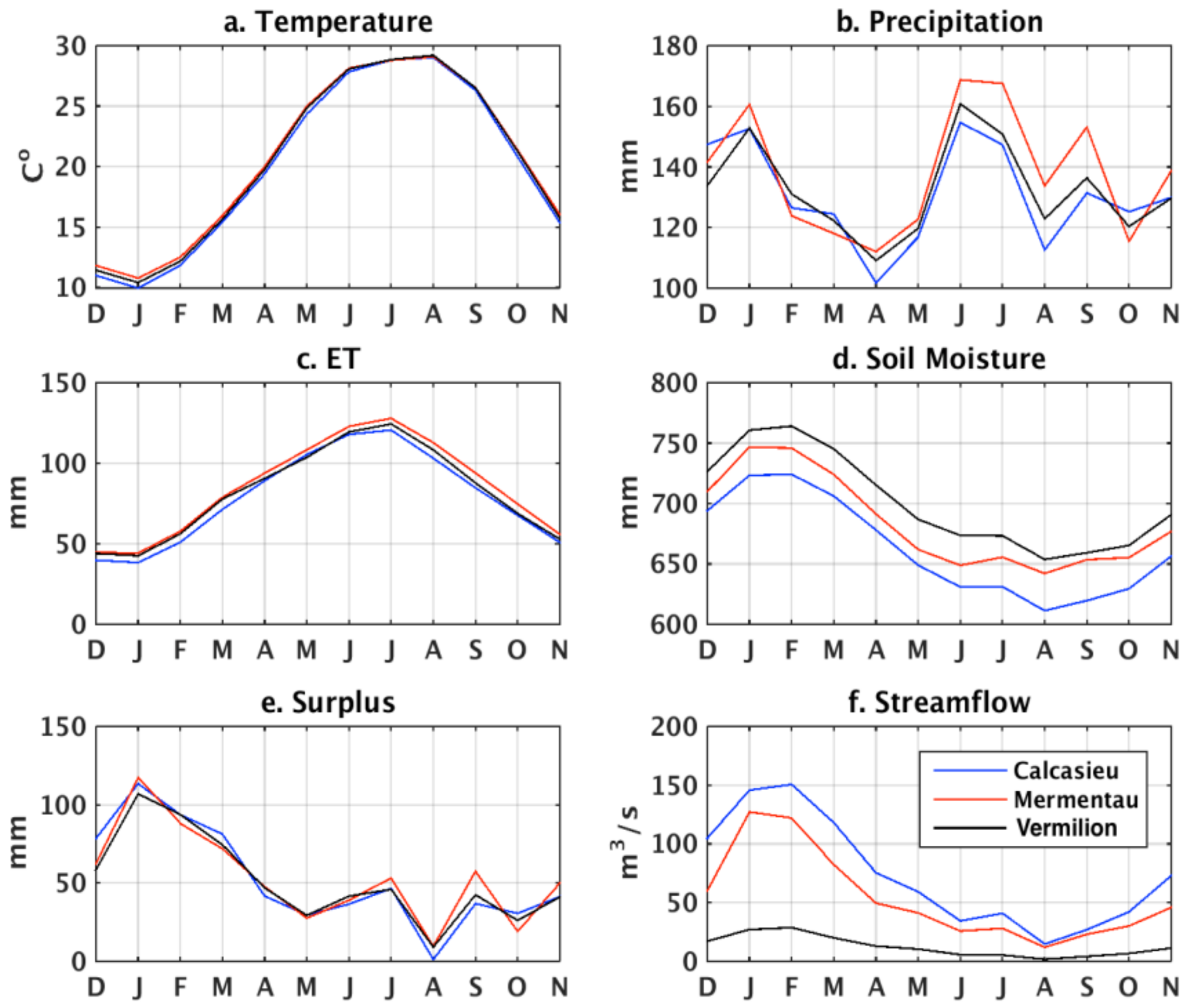
3.2. Temporal Variation
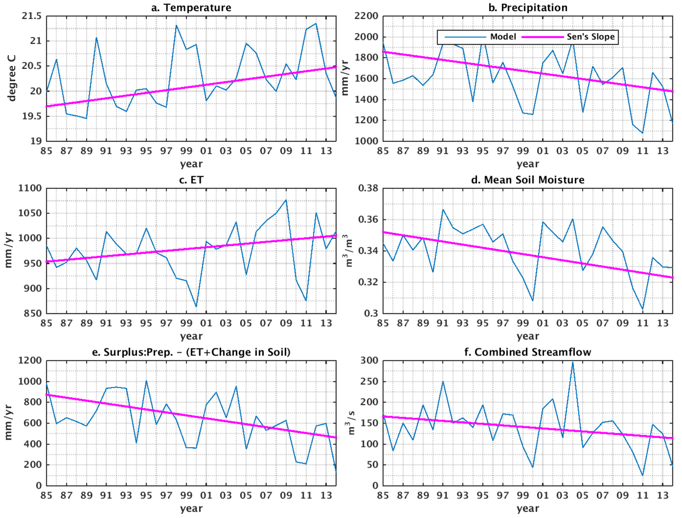
3.3. Trend Analysis
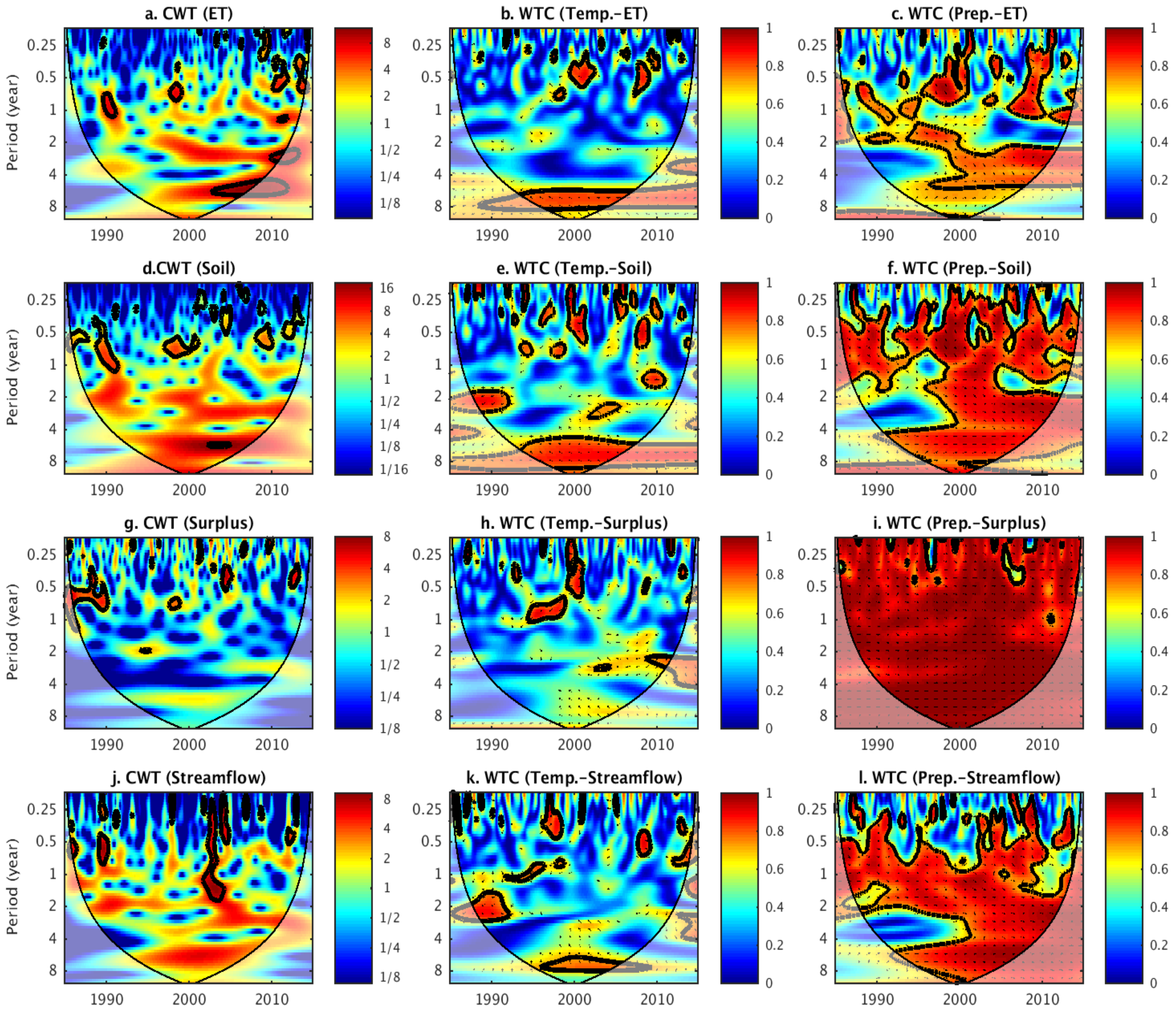
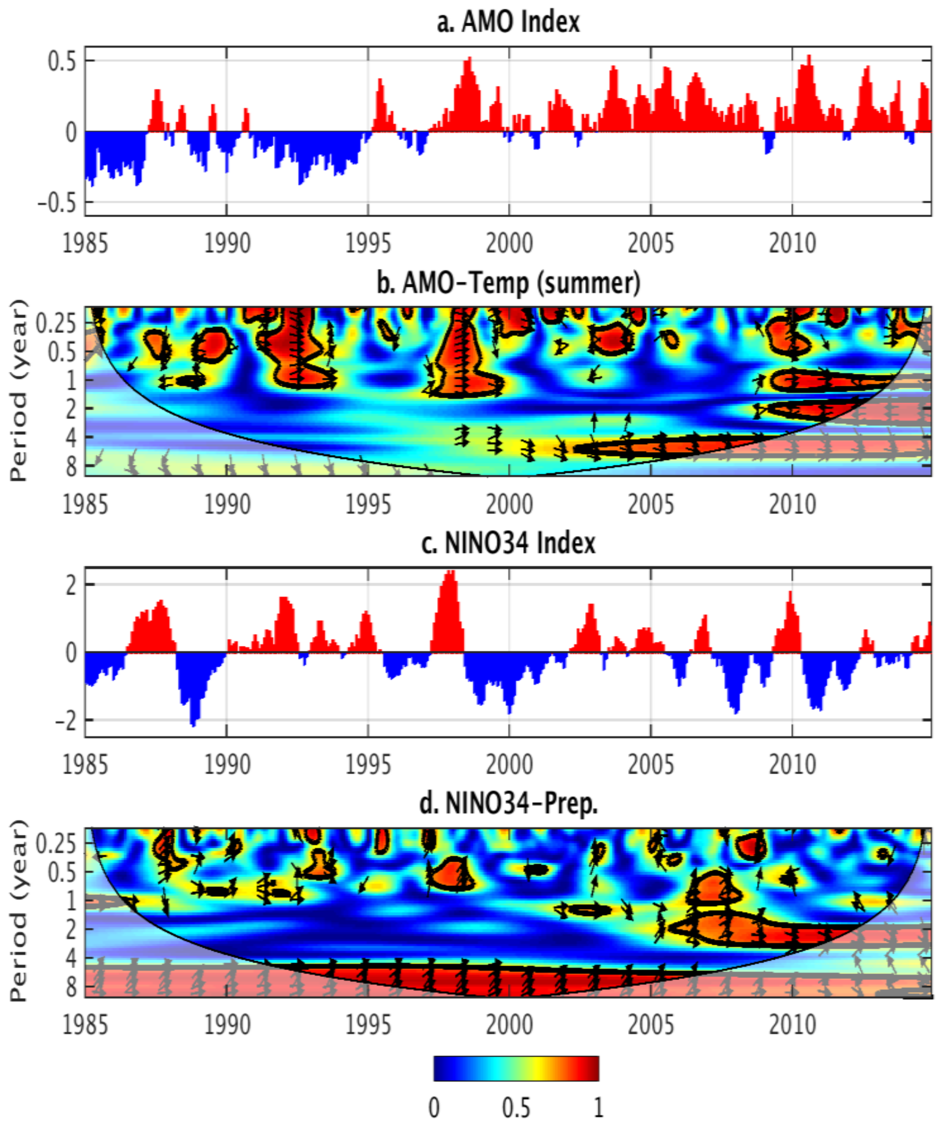
3.4. Wavelet Analysis
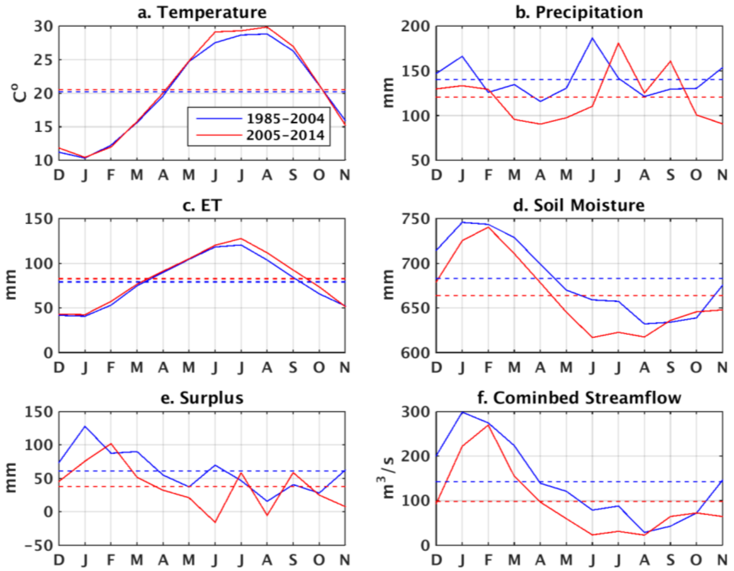
4. Discussion
5. Conclusions
Supplementary Materials
Author Contributions
Funding
Acknowledgments
Conflicts of Interest
References
- Vörösmarty, C.J.; Green, P.; Salisbury, J.; Lammers, R.B. Global water resources: Vulnerability from climate change and population growth. Science 2000, 289, 284–288. [Google Scholar] [CrossRef] [PubMed]
- McGranahan, G.; Balk, D.; Anderson, B. The rising tide: Assessing the risks of climate change and human settlements in low elevation coastal zones. Environ. Urban. 2007, 19, 17–37. [Google Scholar] [CrossRef]
- Nicholls, R.J.; Cazenave, A. Sea-level rise and its impact on coastal zones. Science 2010, 328, 1517–1520. [Google Scholar] [CrossRef] [PubMed]
- Ferguson, G.; Gleeson, T. Vulnerability of coastal aquifers to groundwater use and climate change. Nat. Clim. Chang. 2012, 2, 342–345. [Google Scholar] [CrossRef]
- Knutson, T.R.; McBride, J.L.; Chan, J.; Emanuel, K.; Holland, G.; Landsea, C.; Held, I.; Kossin, J.P.; Srivastava, A.K.; Sugi, M. Tropical cyclones and climate change. Nat. Geosci. 2010, 3, 157–163. [Google Scholar] [CrossRef]
- Powell, E.J.; Keim, B.D. Trends in daily temperature and precipitation extremes for the Southeastern United States: 1948–2012. J. Clim. 2015, 28, 1592–1612. [Google Scholar] [CrossRef]
- Keim, B.D.; Faiers, G.E.; Muller, R.A.; Grymes, J.M.; Rohli, R.V. Long-term trends of precipitation and runoff in Louisiana, USA. Int. J. Climatol. 1995, 15, 531–541. [Google Scholar] [CrossRef]
- Keim, B.D.; Fontenot, R.; Tebaldi, C.; Shankman, D. Hydroclimatology of the US Gulf Coast under global climate change scenarios. Phys. Geogr. 2011, 32, 561–582. [Google Scholar] [CrossRef]
- Enfield, D.B.; Mestas-Nuñez, A.M.; Trimble, P.J. The Atlantic Multidecadal Oscillation and its relation to rainfall and river flows in the continental US. Geophys. Res. Lett. 2001, 28, 2077–2080. [Google Scholar] [CrossRef]
- McCabe, G.J.; Palecki, M.A.; Betancourt, J.L. Pacific and Atlantic Ocean influences on multidecadal drought frequency in the United States. Proc. Natl. Acad. Sci. USA 2004, 101, 4136–4141. [Google Scholar] [CrossRef] [PubMed]
- Knight, J.R.; Folland, C.K.; Scaife, A.A. Climate impacts of the Atlantic multidecadal oscillation. Geophys. Res. Lett. 2006, 33, L17706. [Google Scholar] [CrossRef]
- Sanchez-Rubio, G.; Perry, H.M.; Biesiot, P.M.; Johnson, D.R.; Lipcius, R.N. Oceanic–atmospheric modes of variability and their influence on riverine input to coastal Louisiana and Mississippi. J. Hydrol. 2011, 396, 72–81. [Google Scholar] [CrossRef]
- Nohara, D.; Kitoh, A.; Hosaka, M.; Oki, T. Impact of climate change on river discharge projected by multimodel ensemble. J. Hydrometeorol. 2006, 7, 1076–1089. [Google Scholar] [CrossRef]
- Rosen, T.; Xu, Y. Riverine sediment inflow to Louisiana Chenier Plain in the Northern Gulf of Mexico. Estuar. Coast. Shelf Sci. 2011, 95, 279–288. [Google Scholar] [CrossRef]
- Xia, Y.; Mitchell, K.; Ek, M.; Sheffield, J.; Cosgrove, B.; Wood, E.; Luo, L.; Alonge, C.; Wei, H.; Meng, J.; et al. Continental-scale water and energy flux analysis and validation for the North American Land Data Assimilation System project phase 2 (NLDAS-2): 1. Intercomparison and application of model products. J. Geophy. Res. Atmos. 2012, 117. [Google Scholar] [CrossRef]
- Gochis, D.J.; Yu, W.; Yates, D.N. The WRF-Hydro Model Technical Description and User’s Guide, Version 3.0. NCAR Technical Document. 2015, p. 120. Available online: http://www.ral.ucar.edu/projects/wrf_hydro/ (accessed on 1 May 2018).
- Gochis, D.; Schumacher, R.; Friedrich, K.; Doesken, N.; Kelsch, M.; Sun, J.; Ikeda, K.; Lindsey, D.; Wood, A.; Dolan, B.; et al. The great Colorado flood of September 2013. Bull. Am. Meteorol. Soc. 2015, 96, 1461–1487. [Google Scholar] [CrossRef]
- Turner, R.E. Wetland loss in the northern Gulf of Mexico: Multiple working hypotheses. Estuaries 1997, 20, 1–13. [Google Scholar] [CrossRef]
- Coastal Protection and Restoration Authority of Louisiana. Fiscal Year 2011 Annual Plan: Integrated Ecosystem Restoration and Hurricane Protection in Coastal Louisiana; Coastal Protection and Restoration Authority of Louisiana: Baton Rouge, LA, USA, 2010.
- Baker, N.T. Hydrologic Features and Processes of the Vermilion River, Louisiana. In Water-Resources Investigations Report 88-4019; United States Geological Survey: Reston, VA, USA, 1988. [Google Scholar]
- Niu, G.-Y.; Yang, Z.L.; Mitchell, K.E.; Chen, F.; Ek, M.B.; Barlage, M.; Kumar, A.; Manning, K.; Niyogi, D.; Rosero, E.; et al. The community Noah land surface model with multiparameterization options (Noah-MP): 1. Model description and evaluation with local-scale measurements. J. Geophys. Res. Atmos. 2011, 116. [Google Scholar] [CrossRef]
- Chen, F.; Manning, K.W.; LeMone, M.A.; Trier, S.B.; Alfieri, J.G.; Roberts, R.; Tewari, M.; Niyogi, D.; Horst, T.W.; Oncley, S.P.; et al. Description and evaluation of the characteristics of the NCAR high-resolution land data assimilation system. J. Appl. Meteorol. Climatol. 2007, 46, 694–713. [Google Scholar] [CrossRef]
- Sampson, K.; Gochis, D.J. WRF Hydro GIS Pre-Processing Tools; Version 2.2; National Center for Atmospheric Research, Research Application Laboratory: Boulder, CO, USA, 2015. [Google Scholar]
- McKay, L.; Bondelid, T.; Dewald, T.; Johnston, J.; Moore, R.; Rea, A. NHDPlus Version 2: User Guide; National Operational Hydrologic Remote Sensing Center: Washington, DC, USA, 2012.
- Wigmosta, M.S.; Vail, L.W.; Lettenmaier, D.P. A distributed hydrology-vegetation model for complex terrain. Water Resour. Res. 1994, 30, 1665–1679. [Google Scholar] [CrossRef]
- Wigmosta, M.S.; Lettenmaier, D.P. A comparison of simplified methods for routing topographically driven subsurface flow. Water Resour. Res. 1999, 35, 255–264. [Google Scholar] [CrossRef]
- Julien, P.Y.; Saghafian, B.; Ogden, F.L. Raster-based hydrologic modeling of spatially–varied surface runoff. J. Am. Water Resour. Assoc. 1995, 31, 523–536. [Google Scholar] [CrossRef]
- Ogden, F.; Sharif, H.O.; Senarath, S.U.S.; Smith, J.A.; Baeck, M.L.; Richardson, J.R. Hydrologic analysis of the Fort Collins, Colorado, flash flood of 1997. J. Hydrol. 2000, 228, 82–100. [Google Scholar] [CrossRef]
- Nash, J.E.; Sutcliffe, J.V. River flow forecasting through conceptual models part I—A discussion of principles. J. Hydrol. 1970, 10, 282–290. [Google Scholar] [CrossRef]
- Gupta, H.V.; Sorooshian, S.; Yapo, P.O. Status of automatic calibration for hydrologic models: Comparison with multilevel expert calibration. J. Hydrol. Eng. 1999, 4, 135–143. [Google Scholar] [CrossRef]
- Singh, J.; Knapp, H.V.; Arnold, J.; Demissie, M. Hydrological modeling of the Iroquois River watershed using HSPF and SWAT. J. Am. Water Resour. Assoc. 2005, 41, 343–360. [Google Scholar] [CrossRef]
- Moriasi, D.N.; Arnold, J.G.; Van Liew, M.W.; Bingner, R.L.; Harmel, R.D.; Veith, T.L. Model evaluation guidelines for systematic quantification of accuracy in watershed simulations. Trans. ASABE 2007, 50, 885–900. [Google Scholar] [CrossRef]
- Cai, X.; Yang, Z.-L.; David, C.H.; Niu, G.-Y.; Rodell, M. Hydrological evaluation of the Noah-MP land surface model for the Mississippi River Basin. J. Geophys. Res. Atmos. 2014, 119, 23–38. [Google Scholar] [CrossRef]
- Chen, F.; Mitchell, K.; Schaake, J.; Xue, Y.; Pan, H.; Koren, V.; Duan, Q.Y.; Ek, M.; Betts, A. Modeling of land surface evaporation by four schemes and comparison with FIFE observations. J. Geophys. Res. Atmos. 1996, 101, 7251–7268. [Google Scholar] [CrossRef]
- Mu, Q.; Zhao, M.; Running, S.W. Improvements to a MODIS global terrestrial evapotranspiration algorithm. Remote Sens. Environ. 2011, 115, 1781–1800. [Google Scholar] [CrossRef]
- Hipel, K.W.; McLeod, A.I. Time Series Modelling of Water Resources and Environmental Systems; Elsevier: London, UK, 1994. [Google Scholar]
- Libiseller, C.; Grimvall, A. Performance of partial Mann–Kendall tests for trend detection in the presence of covariates. Environmetrics 2002, 13, 71–84. [Google Scholar] [CrossRef]
- Sen, P.K. Estimates of the regression coefficient based on Kendall’s tau. J. Am. Stat. Assoc. 1968, 63, 1379–1389. [Google Scholar] [CrossRef]
- Pettitt, A. A non-parametric approach to the change-point problem. Appl. Stat. 1979, 28, 126–135. [Google Scholar] [CrossRef]
- Pohlert, T. Non-Parametric Trend Tests and Change-Point Detection, CC BY-ND 4.0. 2016.
- Grinsted, A.; Moore, J.C.; Jevrejeva, S. Application of the cross wavelet transform and wavelet coherence to geophysical time series. Nonlinear Process. Geophys. 2004, 11, 561–566. [Google Scholar] [CrossRef]
- Carey, S.K.; Tetzlaff, D.; Buttle, J.; Laudon, H.; McDonnell, J.; McGuire, K.; Seibert, J.; Soulsby, C.; Shanley, J. Use of color maps and wavelet coherence to discern seasonal and interannual climate influences on streamflow variability in northern catchments. Water Resour. Res. 2013, 49, 6194–6207. [Google Scholar] [CrossRef]
- Thornthwaite, C.W. An approach toward a rational classification of climate. Geogr. Rev. 1948, 38, 55–94. [Google Scholar] [CrossRef]
- Mather, J.R. The Climatic Water Budget in Environmental Analysis; Free Press: Glencoe, IL, USA, 1978. [Google Scholar]
- Subudhi, P.K.; Parami, N.; Materne, M.; Harrison, S. Genetic diversity in smooth cordgrass from brown marsh areas of Louisiana. J. Aquat. Plant Manag. 2008, 46, 60–67. [Google Scholar]
- Van der Wiel, K.; Kapnick, S.B.; Jan van Oldenborgh, G.; Whan, K.; Philip, S.; Vecchi, G.A.; Singh, R.K.; Arrighi, J.; Cullen, H. Rapid attribution of the August 2016 flood-inducing extreme precipitation in south Louisiana to climate change. Hydrol. Earth Syst. Sci. 2017, 21, 897. [Google Scholar] [CrossRef]


| Basin | Area (km2) | Land Use (%) | |||||
|---|---|---|---|---|---|---|---|
| Forest | Shrub/Savanna/Grass | Wetland | Cropland | Urban | Water | ||
| Calcasieu | 15,423 | 41 | 39 | 5 | 11 | 1 | 3 |
| Mermentau | 13,785 | 8 | 28 | 8 | 48 | <1 | 5 |
| Vermilion-Teche | 14,696 | 19 | 18 | 6 | 43 | 1 | 12 |
| Total | 43,904 | 23 | 29 | 6 | 34 | 1 | 6 |
| Basins | Number of Stations | Temperature (Monthly Mean, Unit: °C) | Precipitation (Monthly, Unit: mm) | ||||||||
|---|---|---|---|---|---|---|---|---|---|---|---|
| Station | NDLAS-2 | RSR | NSE | PBIAS | Station | NDLAS | RSR | NSE | PBIAS | ||
| Calcasieu | 12 | 19.79 | 20.01 | 0.11 | 0.99 | −1% | 128.86 | 131.97 | 0.47 | 0.78 | −2% |
| Mermentau | 8 | 20.08 | 20.50 | 0.18 | 0.98 | −2% | 131.78 | 139.15 | 0.54 | 0.71 | −5% |
| Vermilion-Teche | 9 | 20.10 | 20.33 | 0.16 | 0.97 | −1% | 132.58 | 133.56 | 0.54 | 0.71 | −1% |
| Entire Region | 29 | 19.99 | 20.27 | 0.12 | 0.98 | −1% | 131.07 | 134.77 | 0.44 | 0.81 | −3% |
| Basin | Station id | Lon | Lat | Covered Period * | # of Month | Monthly Mean Runoff (m3·s−1) | r | r (for Anomaly) | RSR | NSE | PBIAS |
|---|---|---|---|---|---|---|---|---|---|---|---|
| Calcasieu | 08013000 | −92.673 | 30.996 | 01/85–12/14 | 360 | 21.40 | 0.91 | 0.89 | 0.41 | 0.83 | 3% |
| 08013500 | −92.814 | 30.641 | 01/85–12/14 | 348 | 28.63 | 0.95 | 0.94 | 0.33 | 0.89 | −12% | |
| 08014500 | −92.893 | 30.699 | 01/85–12/14 | 360 | 20.82 | 0.90 | 0.88 | 0.53 | 0.72 | −10% | |
| 08014800 | −93.231 | 30.819 | 09/07–12/14 | 87 | 3.06 | 0.85 | 0.76 | 0.76 | 0.43 | −39% | |
| 08015500 | −92.915 | 30.503 | 01/85–12/14 | 360 | 68.42 | 0.93 | 0.92 | 0.38 | 0.86 | −8% | |
| Mermentau | 08010000 | −92.491 | 30.483 | 01/85–12/14 | 360 | 7.85 | 0.83 | 0.81 | 0.60 | 0.65 | 24% |
| 08012000 | −92.632 | 30.481 | 01/85–12/14 | 360 | 22.66 | 0.89 | 0.87 | 0.47 | 0.78 | 11% | |
| 08012150 | −92.591 | 30.190 | 10/89–12/14 | 292 | 62.28 | 0.85 | 0.83 | 0.56 | 0.68 | 15% | |
| Vermilion-Teche | 07382000 | −92.380 | 31.000 | 01/85–12/14 | 336 | 11.13 | 0.90 | 0.89 | 0.51 | 0.74 | 5% |
| 07382500 ** | −92.056 | 30.618 | 01/85–11/14 | 240 | 27.30 | 0.93 | 0.88 | 0.74 | 0.45 | 56% | |
| 07385700 ** | −91.829 | 30.071 | 01/85–12/14 | 360 | 13.12 | 0.88 | 0.80 | 1.98 | −2.92 | 91% | |
| 07386980 ** | −92.156 | 29.952 | 01/85–12/14 | 339 | 33.55 | 0.72 | 0.63 | 0.96 | 0.07 | 42% |
| River | Variables | Seasonal Mann-Kendall (n = 360 months) | Mann-Kendall (n = 30 year) | Sen’s Slope (n = 30 year) | Pettitt’s Change-Point (n = 30 year) | ||||
|---|---|---|---|---|---|---|---|---|---|
| S Score * | p-Value | S Score * | p-Value | Slope | Intercept | Change Point (Year) | p-Value | ||
| Calcasieu | Ground Temp. | 499 | 0.010 | 123 | 0.029 | 0.025 | 19.469 | 1997 | 0.037 |
| Precipitation | −434 | 0.025 | −59 | 0.301 | −7.344 | 1735.008 | 1997 | 0.762 | |
| ET | 628 | 0.001 | 103 | 0.069 | 1.824 | 913.596 | 2000 | 0.149 | |
| Soil Moisture | −880 | <0.001 | −79 | 0.164 | <−0.001 | 0.342 | 2008 | 0.299 | |
| Surplus | −412 | 0.033 | −109 | 0.054 | −11.028 | 828.732 | 2004 | 0.195 | |
| Streamflow (obs.) | −1178 | <0.001 | −139 | 0.014 | −1.481 | 87.918 | 2004 | 0.042 | |
| Streamflow (model) | −674 | <0.001 | −85 | 0.134 | −1.101 | 87.141 | 2004 | 0.276 | |
| Mermentau | Ground Temp. | 467 | 0.016 | 128 | 0.023 | 0.024 | 19.927 | 1997 | 0.037 |
| Precipitation | −389 | 0.047 | −85 | 0.134 | −10.572 | 1795.056 | 2004 | 0.300 | |
| ET | 392 | 0.043 | 89 | 0.116 | 1.884 | 987.084 | 2000 | 0.111 | |
| Soil Moisture | −788 | <0.001 | −89 | 0.116 | <−0.001 | 0.351 | 2004 | 0.232 | |
| Surplus | −460 | 0.018 | −113 | 0.046 | −12.300 | 836.304 | 2004 | 0.135 | |
| Streamflow (obs) | −498 | 0.010 | −107 | 0.059 | −0.295 | 26.050 | 2004 | 0.090 | |
| Streamflow (model) | −800 | <0.001 | −103 | 0.169 | −0.340 | 25.503 | 2004 | 0.179 | |
| Vermilion-Tech | Ground Temp. | 665 | <0.001 | 154 | 0.006 | 0.030 | 19.685 | 1997 | 0.009 |
| Precipitation | −554 | 0.004 | −143 | 0.113 | −17.604 | 1796.424 | 1995 | 0.056 | |
| ET | 212 | 0.275 | 41 | 0.475 | 0.600 | 972.78 | 2000 | 0.829 | |
| Soil Moisture | −1053 | <0.001 | −131 | 0.020 | <−0.001 | 0.363 | 1997 | 0.062 | |
| Surplus | −580 | 0.003 | −159 | 0.005 | −17.676 | 802.248 | 1995 | 0.045 | |
| Streamflow (obs) | −208 | 0.284 | −35 | 0.544 | −0.044 | 14.124 | 1998 | 0.740 | |
| Streamflow (model) | −604 | 0.002 | −79 | 0.164 | −0.167 | 16.396 | 2004 | 0.214 | |
| 3-basins | Ground Temp. | 567 | 0.003 | 135 | 0.017 | 0.027 | 19.669 | 1997 | 0.023 |
| Precipitation | −464 | 0.017 | −113 | 0.046 | −13.08 | 1870.968 | 2004 | 0.254 | |
| ET | 414 | 0.032 | 93 | 0.101 | 1.788 | 951.96 | 2000 | 0.148 | |
| Soil Moisture | −919 | <0.001 | −93 | 0.101 | <−0.001 | 0.353 | 2004 | 0.233 | |
| Surplus | −476 | 0.014 | −147 | 0.009 | −14.124 | 886.848 | 2004 | 0.047 | |
| Streamflow ** (obs) | −912 | <0.001 | −123 | 0.030 | −1.943 | 126.570 | 2004 | 0.053 | |
| Streamflow (model) | −712 | <0.001 | −91 | 0.108 | −1.425 | 115.498 | 2004 | 0.254 | |
© 2018 by the authors. Licensee MDPI, Basel, Switzerland. This article is an open access article distributed under the terms and conditions of the Creative Commons Attribution (CC BY) license (http://creativecommons.org/licenses/by/4.0/).
Share and Cite
Xue, Z.G.; Gochis, D.J.; Yu, W.; Keim, B.D.; Rohli, R.V.; Zang, Z.; Sampson, K.; Dugger, A.; Sathiaraj, D.; Ge, Q. Modeling Hydroclimatic Change in Southwest Louisiana Rivers. Water 2018, 10, 596. https://doi.org/10.3390/w10050596
Xue ZG, Gochis DJ, Yu W, Keim BD, Rohli RV, Zang Z, Sampson K, Dugger A, Sathiaraj D, Ge Q. Modeling Hydroclimatic Change in Southwest Louisiana Rivers. Water. 2018; 10(5):596. https://doi.org/10.3390/w10050596
Chicago/Turabian StyleXue, Z. George, David J. Gochis, Wei Yu, Barry D. Keim, Robert V. Rohli, Zhengchen Zang, Kevin Sampson, Aubrey Dugger, David Sathiaraj, and Qian Ge. 2018. "Modeling Hydroclimatic Change in Southwest Louisiana Rivers" Water 10, no. 5: 596. https://doi.org/10.3390/w10050596
APA StyleXue, Z. G., Gochis, D. J., Yu, W., Keim, B. D., Rohli, R. V., Zang, Z., Sampson, K., Dugger, A., Sathiaraj, D., & Ge, Q. (2018). Modeling Hydroclimatic Change in Southwest Louisiana Rivers. Water, 10(5), 596. https://doi.org/10.3390/w10050596