Waves and Currents at a River Mouth: The Role of Macrovortices, Sub-Grid Turbulence and Seabed Friction

Abstract

Numerical experiments of wave-current interaction have been performed to investigate the evolution and dissipation of horizontal large-scale vortical structures generated by differential wave breaking and current shearing at river mouths. Specific focus is on the role played by turbulence of scales smaller than the water depth and by seabed friction on the dissipation of the mentioned macrovortices. The analysis reveals two regions of turbulence generation: at the river mouth, and along the curved seaward boundary of the shoal. In the latter zone, macrovortices are formed due to differential wave breaking induced by the sudden variation in water depth and enhanced by opposing currents which favour wave steepening. Such vortices are then advected towards the shore. Among the dissipative mechanisms, dissipation induced by seabed friction is deemed dominant, in particular in the most shallow waters of the shoal. Sub-grid turbulence dissipation, conversely, is more efficient offshore, although exerting some effect also over the shoal when supported by the continuous action of waves.

1. Introduction

At estuaries, river mouths and inlets in a broader sense, waves and outflowing currents give rise to a very wide spectrum of interactions, which, in turn, has effects on the hydrodynamics and morphology of coastal and estuarine environments. Notwithstanding its relevance, though, this strongly nonlinear interplay is still far to be fully understood, and increasing research efforts have been spent over the last decades to study the phenomena connected with wave-current interactions.

A common and easily detectable feature of interacting waves and currents is wave blocking, an occurrence in which the incoming waves are gradually blocked (with part of their energy reflected back to the open sea) by a current flowing in the opposite direction [1,2]. Wave blocking can considerably reduce the energy of sea waves penetrating the river mouth or estuary, since it leads to local wave steepening and breaking and global energy dissipation. The wave frequency spectrum also experiences a downshift, with the high-frequency energy of wind waves being both dissipated by breaking and partially transferred to low-frequency components such as infragravity waves [3]. Currents themselves are also modified by the interaction with waves; experimental investigations have shown that, because of opposing waves, the current velocity profile loses its typical logarithmic shape, with the current strength decreasing near the bottom and slightly increasing near the mean water level [4]. The effects of waves on the current profiles is also highly dependent on the propagation angle of the waves with respect to the current [5]. In the light of the above, it is clear that the coastal areas located at the convergence of marine and riverine forcings are regions of extreme complexity and their study via experimental and observational means is very difficult. The analysis of the dynamics of wave-current interaction at river mouths has seen a notable increase in recent years thanks to the increasing use of numerical models (e.g., [6,7,8,9]).

Coastal environments where waves and currents coexist are also characterized by a high level of turbulence, which promotes water mixing in both vertical and horizontal directions. Turbulence at the mouth of rivers and in the nearby shallow areas is often supported by large-scale, coherent vortical structures with rotation axis perpendicular to the seabed, commonly known as macrovortices [10,11]. Within a shallow-water framework, large eddies are seen to gradually form after the rearrangement of the vorticity field [12], generated because of wave breaking spatial unevenness due to varying topography in both cross-shore and alongshore directions and also because of the mentioned wave-current interaction. Differential wave breaking leads to breakers of finite length and injection of vorticity at the lateral edges of the breaker [10,13]. Finite-length breakers leading to vorticity generation are also likely to occur because of variabilities in the incoming wave field, or in the presence of cross-sea, i.e., several wave trains approaching the shore from different directions [14]. Finite-length breakers are a source of considerable vorticity $\omega$ that is injected into the fluid [15]; assuming, for the sake of simplicity, a bore (shock discontinuity) with a straight and finite front propagating in the x-direction, so that the y-direction is the cross-flow direction, the amount of potential vorticity generated across the jump or bore, $\mathsf{\Delta }\Omega$, may be evaluated as

$$\mathsf{\Delta }\Omega =-{\left[\frac{2d_2}{g{d}_1\left(d_1+d_2\right)}\right]}^{\frac{1}{2}}\frac{\mathrm{d}{E}_d}{\mathrm{d}y},$$

(1)

where $\Omega =\omega /d$ is the potential vorticity, $d_1$ and $d_2$ are the water depths upstream and downstream of the shock, respectively, and $E_d$ is the specific rate of energy dissipation, which is strictly related to the jump in water height across the shock:

$$E_d=\frac{{\left[d_2-d_1\right]}^3}{4d_1{d}_2}.$$

(2)

According to relation (1), potential vorticity is generated wherever there is a large cross-flow gradient in $E_d$ and, hence, an abrupt cross-flow change in $\left(d_2-d_1\right)$ [16,17]. This situation often happens at the edges of finite-length breakers.

Once macrovortices are well-formed thanks to the reorganization of injected vorticity, they are often advected towards the shore by the action of waves and self-advection, this forcing the vortex to move along the isobaths [10].

A number of studies ascertained that macrovortices are a strong agent in several phenomena and processes occurring in the nearshore, such as flow mixing [18,19,20], entrainment and distribution of sediment [21,22] and advection of passive tracers [23]. As a natural consequence, macrovortices are crucial in defining the geomorphological response of many environments, such as barred beaches [15], riverine systems [24,25,26] and compound channels [27,28]. Some recent studies [29,30,31] also highlighted the role both of river jet instability and of macrovortices for the morphological evolution of estuarine and deltaic structures.

Although a complete representation of turbulent motions at all time and space scales requires important computational efforts, a simplified yet suitable description of the underlying structure of macrovortices can be achieved by means of relatively simple numerical models, such as depth-averaged solvers based on the nonlinear shallow water equations (NSWEs). These models neglect the vertical structure of the described flows by integrating the flow quantities over the water depth, but are still efficient tools to catch the relevant features of wave-current interactions and 2-dimensional large-scale vorticity.

Such simplified models can be further complemented by coupling with Large Eddy Simulation (LES) models to improve their capability of describing vortical flows [26,32,33,34]. In a LES approach, only the “large” turbulent motions, i.e., those occurring at a length scale greater than a predefined filter size (usually taken as the computational grid size), is resolved exactly. The dissipative effect of 3D turbulence occurring at length scales smaller than the flow depth, the so-called “sub-grid scale”, is accounted for by suitable Sub-Grid Scale (SGS) closure models that connect the physical properties of small-scale turbulence with those of the mean flow field [35]. LES schemes for the modeling of vorticity and turbulence have received considerable research attention over the last decades (see, as examples, [26,32,34]) and have been successfully applied to simulate vortical and turbulent patterns in fluvial-like flows [24,28,36]. LES has been proven particularly appropriate to model vortical structures that are generated by shear instabilities within the flow [37]. A LES approach has been adopted to describe frictional effects and jet instability in the work of Canestrelli et al. [30], although their study neglected the effects of wind waves.

The purpose of the present work is to investigate the main mechanisms of flow mixing, with focus on macrovortices, in a simplified river mouth environment, and to better understand the role of seabed friction and sub-grid-scale turbulence in draining energy from such macrovortices. This is done through a parametric, numerical analysis of wave-current interactions performed with a depth-averaged shallow water solver. The effect of frictional dissipation is introduced through a classical Chezy-like formulation for bed stresses; dissipation by sub-grid turbulence is accounted for through a simple horizontal LES (HLES) model. The main vortical and turbulent patterns are therefore observed and discussed.

The paper is organized as follows. In Section 2 a brief description of the numerical framework in use is presented. Section 3 is devoted to a description of the numerical simulations, the main findings of which are illustrated and discussed in Section 4. Concluding remarks are finally given in Section 5.

2. Materials and Methods

2.1. The Nonlinear Shallow Water Equations: The Analytics

The nonlinear shallow water equations are a set of depth-averaged, hyperbolic equations which describes the conservation of mass and momentum in shallow waters. For a more complete treatment of the problem, the standard NSWEs are complemented with additional terms accounting for flow dissipation due to bottom friction and small-scale turbulent motions.

The system of the NSWEs in non-conservative form is:

$$\begin{array}{cc}\hfill d_{,t}+{\left(ud\right)}_{,x}+{\left(vd\right)}_{,y}& =0,\hfill \end{array}$$

(3a)

$$\begin{array}{cc}\hfill u_{,t}+u{u}_{,x}+v{u}_{,y}+g{d}_{,x}& =-g{z}_{b,x}-B_x+F_x,\hfill \end{array}$$

(3b)

$$\begin{array}{cc}\hfill v_{,t}+u{v}_{,x}+v{v}_{,y}+g{d}_{,y}& =-g{z}_{b,y}-B_y+F_y,\hfill \end{array}$$

(3c)

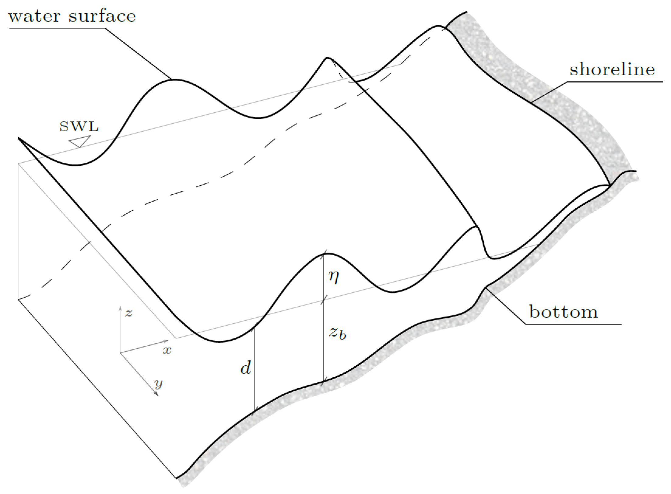
where $\left(x,y,z\right)$ is an orthogonal Cartesian system of spatial coordinates and t represents time. The cross-shore x-coordinate points toward the shore and has its origin at the seaward boundary of the domain of interest (see Figure 1). The datum for the vertical coordinate z is located at the still water level $z=0$. $\mathbf{v}=\left(u,v\right)$ is the vector of the depth-averaged velocities; $d=\eta -z_b$ is the water depth, where $\eta$ is the elevation of the water surface and $z_b$ is the seabed location, both measured from the still water level; g is the acceleration of gravity. Subscripts after commas represent partial differentiation with respect to space or time.

The terms $B_x$ and $B_y$ appearing at the right-hand side of Equations (3b) and (3c) represent the contributions due to seabed friction. When a Chezy-type formulation is used for modelling bed shear stresses, $B_x$ and $B_y$ are defined as follows:

$$B_x=c_{\tau }\frac{\left|\mathbf{v}\right|u}{d}\mathrm{and}{B}_y=c_{\tau }\frac{\left|\mathbf{v}\right|v}{d},$$

(4)

where $c_{\tau }$ is the dimensionless Chezy friction coefficient, usually of order ${10}^{-2}–{10}^{-3}$ [38].

For the purposes of our simulations, $c_{\tau }$ is computed as a function of the initial water depth, using the formulation proposed by van Rijn [39] in case of a hydraulically rough flow:

$$c_{\tau }=\frac{g}{{\left(18log\frac{12d}{k_s}\right)}^2},$$

(5)

where $k_s$ is the bed roughness.

The additional terms $F_x$ and $F_y$ here account for the viscous dissipation due to sub-grid turbulence, i.e., the turbulence that develops at length scales smaller than the water depth and thus not directly resolved. The friction terms $B_x$ and $B_y$ and the viscous dissipation terms $F_x$ and $F_y$ are included among the source terms as they are part of a specific “source” system, as described in the following.

The description of turbulent structures with scales smaller than the water depth is performed by means of a Horizontal Large Eddy Simulation (HLES) model to the likes of those adopted for numerical applications in riverine environments (e.g., [24,28,36,40]). Therefore, only the “large” turbulent motions, i.e., those occurring at a length scale greater than a predefined filter size (in this case the water depth), are directly resolved. The dissipative effect of turbulence at sub-grid scales (SGS) is usually accounted for with appropriate models that link the properties of “small” turbulence to those of the resolved flow. Approaches like this are, in fact, suitable for implementation in depth-averaged solvers, since they lump all the complex mechanisms related to sub-grid turbulence in a simple model in which only mean properties are explicitly used. Of course, a proper physical description of 3D turbulence and all related phenomena is hindered in depth-averaged models, which neglect the essential contibution of vertical velocities and gradients to the development of turbulence. In spite of this, simplified approaches, such as HLES, can still be used satisfactorily to reach a suitable broad description of such complex mechanisms.

An SGS model based on the variable eddy viscosity formulation proposed by Grosso et al. [41] is used in our solver. To implement it, the momentum balance Equations (3b) and (3c) are complemented with terms $F_x$ and $F_y$, representing the dissipative body forces due to the effects of sub-grid turbulence. They are introduced with a typical Laplacian-type formulation as in the following:

$$F_x=\frac{{\left(d{T}_{xx}\right)}_{,x}+{\left(d{T}_{xy}\right)}_{,y}}{d},$$

(6)

$$F_y=\frac{{\left(d{T}_{xy}\right)}_{,x}+{\left(d{T}_{yy}\right)}_{,y}}{d}.$$

(7)

$T_{xx}$, $T_{yy}$ and $T_{xy}$ are the components of the Reynolds stress tensor for turbulent flows, for which a simple closure is considered [24]:

$$T_{xx}=2{\nu }_T{u}_{,x},T_{yy}=2{\nu }_T{v}_{,y},T_{xy}={\nu }_T\left(u_{,y}+v_{,x}\right),$$

(8)

where ${\nu }_T$ is a depth-averaged effective eddy viscosity, defined as a function of the water depth:

$${\nu }_T=\lambda g^{1/2}{d}^{3/2}.$$

(9)

Such eddy viscosity formulation is clearly compatible with the shallow-water approach of the model, as the velocity scale is taken to be the phase speed of waves in shallow waters, i.e., $\sqrt{gd}$ = $g^{1/2}{d}^{1/2}$, and the length scale is the water depth d.

From an operative point of view, Expressions (6) and (7) are included in the source terms along with the bed friction terms $B_x$ and $B_y$, and used to solve the “source” problem (20). Implementing a second-order centered difference scheme to discretize problem (20) over a time step $\mathsf{\Delta }t$, the following expressions for the depth-averaged velocities u and v at mesh node $\left(i,j\right)$ are obtained:

$$u_{i,j}^{n+1}=u_{i,j}^n+{\nu }_T\mathsf{\Delta }t\left[2u_{,xx}+u_{,yy}+v_{,xy}\right]+\frac{{\nu }_T}{d}\mathsf{\Delta }t\left[5d_{,x}{u}_{,x}+\frac{5}{2}{d}_{,y}{u}_{,y}+\frac{5}{2}{d}_{,y}{v}_{,x}\right],$$

(10)

$$v_{i,j}^{n+1}=v_{i,j}^n+{\nu }_T\mathsf{\Delta }t\left[2v_{,yy}+v_{,xx}+u_{,xy}\right]+\frac{{\nu }_T}{d}\mathsf{\Delta }t\left[5d_{,y}{v}_{,y}+\frac{5}{2}{d}_{,x}{u}_{,y}+\frac{5}{2}{d}_{,x}{v}_{,x}\right].$$

(11)

Through Expressions (10) and (11), the values of the depth-averaged velocities $u_{i,j}$ and $v_{i,j}$ are “corrected” by the viscous contributions, to give account of the effect of sub-grid turbulence. The presence and size of such “correction” is determined by the value of the calibration parameter $\lambda$ appearing in the definition of the variable eddy viscosity (9). If $\lambda =0$, the turbulent sub-grid scales are not modeled and the HLES technique is deactivated: the dissipative terms (6) and (7) are not included in the numerical model and the corrective contribution due to viscosity in (10) and (11) is not present, the only corrections being those due to friction. A value of $\lambda \ne 0$ activates the HLES terms and includes their dissipative effects into the numerical solution. When solving Equations (10) and (11), it is assumed that the water depth d is constant, hence the only flow variables that effectively change are the velocities $u_{i,j}$ and $v_{i,j}$. A conservative form of Equations (10) and (11), in line with the use of a conservative formulation for the NSWE system detailed in the following, is therefore not required. The HLES formulation explained above has been successfully tested and validated against experimental evidence in earlier works (e.g., [41,42,43]).

2.1.1. Dimensional Analysis

We now perform a dimensional analysis of the terms of system (3), useful for an introductory assessment of the role of frictional and viscous dissipation forces. By defining a length scale for horizontal distances $L_0$ and a length scale for vertical distances $d_0$, a reference velocity $\sqrt{g{d}_0}$ and a time scale $t_0=L_0/\left(g{d}_0\right)$ can be derived. The dimensionless forms (labeled with a tilde) of the variables appearing in system (3) are then defined as follows:

$$\tilde{x}=\frac{x}{L_0},\tilde{y}=\frac{y}{L_0},\tilde{t}=t\frac{\sqrt{g{d}_0}}{L_0},$$

(12a)

$$\tilde{u}=\frac{u}{\sqrt{g{d}_0}},\tilde{v}=\frac{v}{\sqrt{g{d}_0}},\tilde{d}=\frac{d}{d_0},{\tilde{z}}_b=\frac{z_b}{d_0},{\tilde{\nu }}_T=\frac{{\nu }_T}{\sqrt{g{d}_0}{d}_0},$$

(12b)

$${\tilde{T}}_{xx}=T_{xx}\frac{L_0}{g{d}_0^2},{\tilde{T}}_{yy}=T_{yy}\frac{L_0}{g{d}_0^2},{\tilde{T}}_{xy}=T_{xy}\frac{L_0}{g{d}_0^2}.$$

(12c)

The NSWE system (3), expanded by means of Equations (4), (6) and (7), is thus made dimensionless with scales (12):

$$\begin{array}{cc}{\tilde{d}}_{,\tilde{t}}+{\left(\tilde{u}\tilde{d}\right)}_{,\tilde{x}}+{\left(\tilde{v}\tilde{d}\right)}_{,\tilde{y}}=0,\hfill & \hfill (\mathrm{13a})\\ {\tilde{u}}_{,\tilde{t}}+\tilde{u}{\tilde{u}}_{,\tilde{x}}+\tilde{v}{\tilde{u}}_{,\tilde{y}}+{\tilde{d}}_{,\tilde{x}}=-g{\tilde{z}}_{b,\tilde{x}}-\frac{c_{\tau }}{ϵ}\frac{\left|\tilde{\mathbf{v}}\right|\tilde{u}}{\tilde{d}}+ϵ\frac{{\left(\tilde{d}{\tilde{T}}_{xx}\right)}_{,\tilde{x}}+{\left(\tilde{d}{\tilde{T}}_{xy}\right)}_{,\tilde{y}}}{\tilde{d}},\hfill & \hfill (\mathrm{13b})\\ {\tilde{v}}_{,\tilde{t}}+\tilde{u}{\tilde{v}}_{,\tilde{x}}+\tilde{v}{\tilde{v}}_{,\tilde{y}}+{\tilde{d}}_{,\tilde{y}}=-g{\tilde{z}}_{b,\tilde{y}}-\frac{c_{\tau }}{ϵ}\frac{\left|\tilde{\mathbf{v}}\right|\tilde{v}}{\tilde{d}}+ϵ\frac{{\left(\tilde{d}{\tilde{T}}_{xy}\right)}_{,\tilde{x}}+{\left(\tilde{d}{\tilde{T}}_{yy}\right)}_{,\tilde{y}}}{\tilde{d}},\hfill & \hfill (\mathrm{13c})\end{array}$$

where $ϵ=d_0/L_0$ is a dimensionless parameter defined by the ratio between vertical and horizontal length scales. By inspection of Equations (3b) and (3c), it can be readily seen that $B_x,B_y\propto P_{\tau }=c_{\tau }/ϵ$; the dissipation of flow momentum due to frictional effects is, therefore, more relevant in very shallow waters ($ϵ\ll 1$). On the other hand, the viscous dissipation terms are proportional to $P_{\lambda }=\lambda ϵ$ and are thus dominant over intermediate-to-deep waters, where $ϵ\approx 0.1–1$.

2.2. The Nonlinear Shallow Water Equations: The Numerics

For the NSWE system (3) to be solvable by numerical techniques, it must be cast in a conservative form, which is the most suitable for our purposes since it allows to properly treat flow discontinuities or shocks. Within this numerical framework, in fact, bores and breaking waves can be treated through a synthetic shock-capturing approach by substituting them with jump discontinuities in flow properties. For further details about conservative and non-conservative formulations see [44]. An apt conservative vectorial form of the NSWEs is

$${\mathbf{U}}_{,t}+\mathbf{F}{\left(\mathbf{U}\right)}_{,x}+\mathbf{G}{\left(\mathbf{U}\right)}_{,y}=\mathbf{S}\left(\mathbf{U}\right),$$

(14)

where $\mathbf{U}$ is the vector of conserved variables, which for the chosen conservative form are defined as d, $ud$, and $vd$. $\mathbf{F}\left(\mathbf{U}\right)$ and $\mathbf{G}\left(\mathbf{U}\right)$ are the vectors of fluxes and $\mathbf{S}\left(\mathbf{U}\right)$ is the vector of source terms:

$$\mathbf{U}=\left[\begin{array}{c}d\\ ud\\ vd\end{array}\right],$$

(15)

$$\mathbf{F}\left(\mathbf{U}\right)=\left[\begin{array}{c}ud\\ u^{2}d+\frac{1}{2}g{d}^2\\ uvd\end{array}\right],\mathbf{G}\left(\mathbf{U}\right)=\left[\begin{array}{c}vd\\ uvd\\ v^{2}d+\frac{1}{2}g{d}^2\end{array}\right],$$

(16)

$$\mathbf{S}\left(\mathbf{U}\right)=\left[\begin{array}{c}0\\ -gd{z}_{b,x}-B_{x}d+F_{x}d\\ -gd{z}_{b,y}-B_{y}d+F_{y}d\end{array}\right].$$

(17)

The hyperbolic system of NSWEs (3) is then numerically solved by means of a finite-volume scheme based on the Weighted Averaged Flux (WAF) method developed by Toro [44,45]. The hydrodynamic numerical solver employed in the present work, which is described in detail and validated in [38] as well as through previous experiences with various configurations (e.g., [27,42,43,46,47]), is used to solve the conservative form (14) of the NSWEs and hence update the flow variables $u,v$ and d in a time-marching procedure. The NSWE system (14) is preliminarily split up into two homogeneous, 1-dimensional systems and one “source” system, which are solved separately:

$${\mathbf{U}}_{,t}+\mathbf{F}{\left(\mathbf{U}\right)}_{,x}=0,$$

(18)

$${\mathbf{U}}_{,t}+\mathbf{G}{\left(\mathbf{U}\right)}_{,y}=0,$$

(19)

$${\mathbf{U}}_{,t}=\mathbf{S}\left(\mathbf{U}\right).$$

(20)

The equivalence between the “split” systems and the original one is proven in [44].

Labeling with $H_x$ and $H_y$ the solving schemes for the homogeneous systems (18) and (19), respectively, and with S the scheme for the “source” system (20), the numerical procedure that advances the flow variables from ${\mathbf{U}}^n=\left(u^n,v^n,d^n\right)$ to ${\mathbf{U}}^{n+1}=\left(u^{n+1},v^{n+1},d^{n+1}\right)$, with the bed depth $z_b^n$ remaining constant, is summarised as follows:

$${\mathbf{U}}^{n+1}=\frac{1}{2}\left\{H_{xy}\left[S\left({\mathbf{U}}^n\right)\right]+S\left[H_{xy}\left({\mathbf{U}}^n\right)\right]\right\}$$

(21)

where n is the present integration time and $H_{xy}$ is a numerical operator defined as

$$H_{xy}\left(\mathbf{U}\right)=\frac{1}{2}\left\{H_x\left[H_y\left(\mathbf{U}\right)\right]+H_y\left[H_x\left(\mathbf{U}\right)\right]\right\}.$$

(22)

The arithmetic means figuring in both Equations (21) and (22) are performed to rule out the unavoidable numerical inaccuracies originating from considering 1-dimensional operators separately instead of using a full 2-dimensional approach for the resolution of system (14).

The 1-dimensional schemes $H_x$ and $H_y$ are numerically implemented through a finite-volume discretization. As an example, applying a finite-volume approach to scheme $H_x$, which solves (18), gives the following approximate formula for the unknown averaged vector ${\mathbf{U}}^{n+1}$:

$${\mathbf{U}}_i^{n+1}={\mathbf{U}}_i^n+\frac{\mathsf{\Delta }t}{\mathsf{\Delta }x}\left({\mathbf{F}}_{i-\frac{1}{2}}^{n+\frac{1}{2}}-{\mathbf{F}}_{i+\frac{1}{2}}^{n+\frac{1}{2}}\right)$$

(23)

where i represents the grid point of interest, $\mathsf{\Delta }x$ is the grid size in the x direction, $\mathsf{\Delta }t$ is the time step (automatically determined and adapted according to the mesh size through the CFL condition), and ${\mathbf{F}}_{i\pm \frac{1}{2}}^{n+\frac{1}{2}}$ are unknown numerical flux vectors, to be evaluated via the WAF method.

The “source” system (20) can be easily solved using standard methods for sets of ordinary differential equations. In scheme S the frictional terms $B_x$ and $B_y$ are discretized via a second-order midpoint method. The viscous terms $F_x$ and $F_y$, on the other hand, are second-order discretized and implemented through the HLES model, described in Section 2.1.

2.3. The River Mouth Model

The basic version of the NSWE solver described in the previous section, as presented in [38], accepts a wave input in the form of a time series of both elevation of water surface and water depth-averaged orbital velocity. The input is applied at the grid nodes of the seaward domain boundary. This approach is consistent with the numerical framework, since the forcing of the mentioned quantities is equivalent to imposing the boundary values of the Riemann invariants propagating along the characteristics curves of the NSWEs.

In order to make the solver able to reproduce complex flow configurations typical of estuarine environments, where the incoming waves interact with an outflowing current, the solver is complemented with a simple estuarine model.

A window of “river mouth nodes” or “estuary nodes” can be defined within the landward edge of the computational domain, through which the input river current can enter the domain. The estuary window is defined by the longshore y-coordinate of its center, $y_{m,e}$ (the estuary center x-coordinate, $x_{m,e}$, being automatically assumed as the x-coordinate of the landward domain boundary), and its width $L_e$. The spatial limits of the estuary window are, therefore

$$y_{min,e}=y_{m,e}-\frac{L_e}{2},y_{max,e}=y_{m,e}+\frac{L_e}{2}.$$

(24)

The mesh nodes at the landward domain boundary falling between $y_{min,e}$ and $y_{max,e}$ are labelled as “estuary nodes”. At these nodes, similarly to what happens at the seaward boundary, a time history of current velocity and/or water level elevation is prescribed to simulate the entrance of river discharges into the basin.

The estuarine input is given as a time history for the depth-averaged water velocity ${\mathbf{U}}_b=\left(u_b,v_b\right)$ and water elevation ${\eta }_b$. The values of the time history are equally spaced in time by a constant interval $\mathsf{\Delta }{t}_b$, which does not need to be equal to the time step determined by the solver, as the computation is automatically adapted to satisfy the CFL stability condition, which is varying at each step. To encompass different real-world situations, the estuarine input is allowed to enter at different angles with respect to the basin. To allow for the propagation of the estuary input at a variable angle of incidence, a simple numerical procedure for the evaluation of the boundary condition values to be imposed at estuary nodes has been developed, which is briefly explained in the following.

Two distinct cases may occur: the input may enter the domain perpendicularly to the boundary edge (at an angle $\theta =0$ with respect to the outer-pointing normal to the edge), or obliquely (at an angle $\theta \ne 0$). Although the numerical treatment for the first scenario can be seen as a special case of the procedure used for the second scenario, we treat the two cases separately for clarity.

• Case I: estuary input perpendicular to the boundary ($\theta =0$). All the estuary nodes “read” the same boundary conditions from the time history simultaneously since they are “touched” by the input signal at the same time. Moreover, since the estuary input is perpendicular to the normal of the domain edge, the estuary input velocity ${\mathbf{U}}_b$ is already oriented in the x-direction and has no y-component, so that ${\mathbf{U}}_b=\left(u_b,0\right)$.
  As said previously, the estuarine boundary conditions (in terms of imposed fluid velocity $u_b$ and water elevation ${\eta }_b$) are sampled at a constant interval $\mathsf{\Delta }{t}_b$ that a priori is not the same as the solver-defined, variable time interval $\mathsf{\Delta }t$; therefore, it is likely that the current solution time level t falls between two consecutive time instants $t_m$ and $t_{m+1}$ in the estuary input time series, so that $t_m\le t\le t_{m+1}$. Then the exact values of fluid elevation ${\widehat{\eta }}_b$ and velocity ${\widehat{u}}_b$ to impose at all estuary nodes at the solution level t are then obtained through linear interpolation between the boundary condition values at times $t_m$ and $t_{m+1}$:

  $${\widehat{\eta }}_b={\eta }_{b,m}+\left({\eta }_{b,m+1}-{\eta }_{b,m}\right)\frac{t-t_m}{t_{m+1}-t_m}$$

  (25)

  and

  $${\widehat{u}}_b=u_{b,m}+\left(u_{b,m+1}-u_{b,m}\right)\frac{t-t_m}{t_{m+1}-t_m},$$

  (26)

  where ${\eta }_{b,m}$ and $u_{b,m}$ are the prescribed boundary values for fluid elevation and velocity at time $t_m$ of the input time series, and ${\eta }_{b,m+1}$ and $u_{b,m+1}$ are the same boundary values at time $t_{m+1}$ of the input time series. The extrapolated values ${\widehat{\eta }}_b$ and ${\widehat{u}}_b$, finally, are imposed at all estuary nodes by adding them to the existing values of water depth $d_n$ and velocity $u_n$. The updated values are then carried on to the next solution step, $t_{n+1}=t_n+\mathsf{\Delta }t$. Hence, for the generic estuary node,

  $$d_{n+1}=d_n+{\widehat{\eta }}_b\mathrm{and}{u}_{n+1}=u_n+{\widehat{u}}_b.$$

  (27)
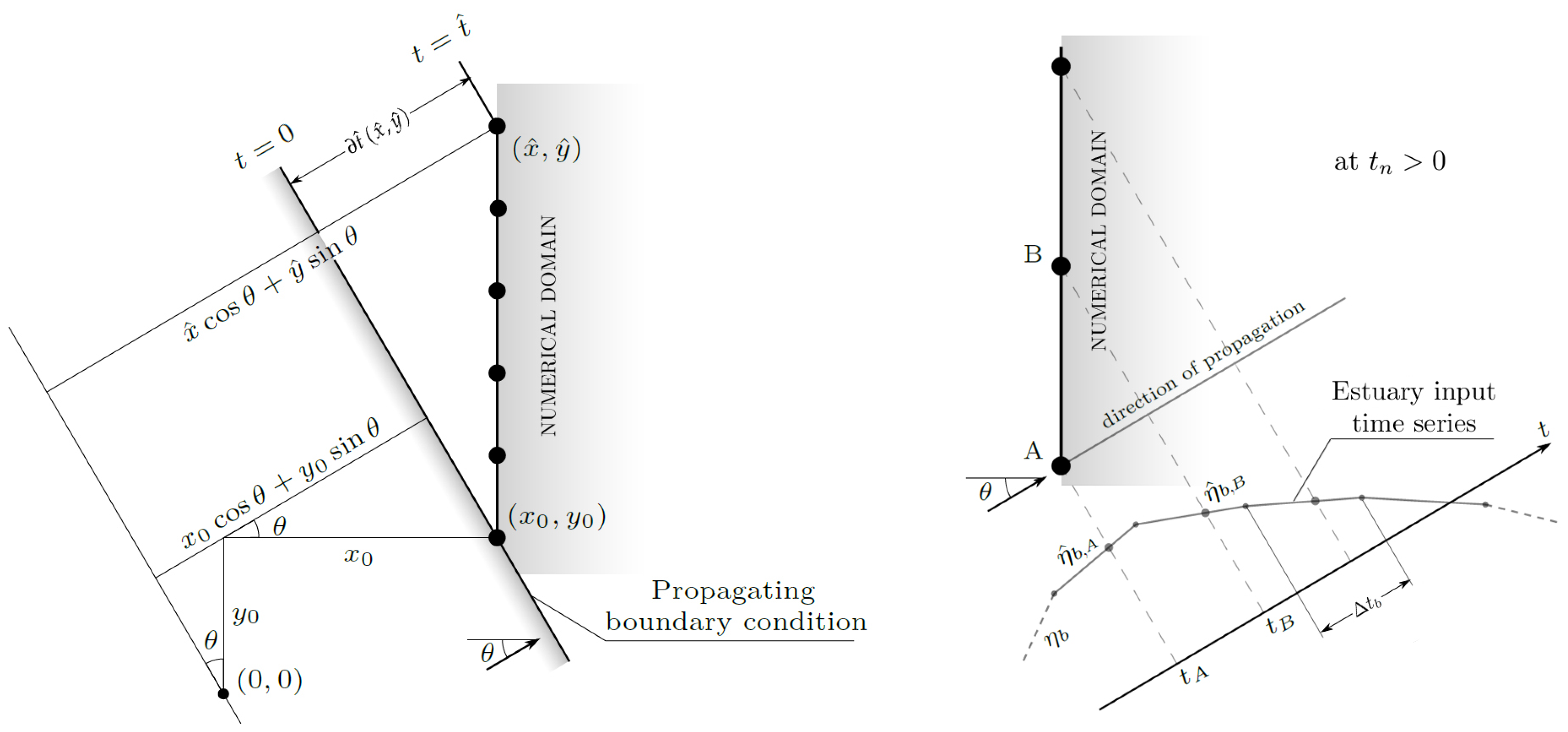
• Case II: estuary input oblique to the boundary ($\theta \ne 0$). Since the fronts of the estuarine input are propagating obliquely, the estuary nodes are “touched” by a single boundary condition value at different times according to the signal propagation velocity (in other terms, at a fixed solution time $t_n$, different estuary nodes “read” different boundary values from the input time history). Moreover, the estuary input fluid velocity ${\mathbf{U}}_b$ is now oriented at an angle with respect to the x-direction, and thus can be decomposed into an x-component, $u_b$, and a y-component, $y_b$. Each component alters the corresponding nodal velocity as effect of the estuarine boundary condition.
  Since each estuary node “reads” different boundary values of water elevation ${\eta }_b$ and velocity ${\mathbf{U}}_b$ at the same solution time, a key problem is to understand which boundary values each node “read”, and how to compute them from the input time history. This is done by assuming that the estuarine input propagates according to the characteristic propagation speed or celerity $\sqrt{gd}$.
  Refer to the left panel in Figure 2. Let $\left(x_0,y_0\right)$ be the coordinates of the first estuary node interested by the estuary input (the “first contact” node hereinafter), and $\left(\widehat{x},\widehat{y}\right)$ the coordinates of another estuary node different from the first. At the start of the numerical simulation ($t_n=0$), the estuary input interests only the “first contact” node. At the following times (solution time levels $t_{n+1}$, $t_{n+2}$…), the input value that only interested the “first contact” node has travelled into the domain (along the direction defined by the angle $\theta$) and perhaps has interested other nodes $\left(\widehat{x},\widehat{y}\right)$ of the estuary window. The time $\partial \widehat{t}$ that a boundary condition value would take to travel from the “first contact” node $\left(x_0,y_0\right)$ to any other estuary node $\left(\widehat{x},\widehat{y}\right)$ along the direction defined by $\theta$ is evaluated with the following formula:

  $$\partial \widehat{t}\left(\widehat{x},\widehat{y}\right)=\frac{\left(\widehat{x}cos\theta +\widehat{y}sin\theta \right)-\left(x_{0}cos\theta +y_{0}sin\theta \right)}{\sqrt{g{d}_0}}.$$

  (28)
  The quantity appearing at the numerator in (28) represents the linear distance between the generic estuary node $\left(\widehat{x},\widehat{y}\right)$ and the “first contact” node $\left(x_0,y_0\right)$, evaluated along the direction defined by $\theta$, i.e., the direction of propagation of the estuary input; this is the “space” covered by the traveling boundary condition. The denominator in (28) is the celerity of the estuary input signal, approximately evaluated using $d_0$, the water depth at the "first contact" node.
  We can now find, for a specific solution time level, which boundary conditions $\left({\widehat{\eta }}_b,{\widehat{\mathbf{U}}}_b\right)$ each estuary node “reads” from the time history. Reference to the right panel in Figure 2 is made in the following. Suppose that at a generic solution time $t_n>0$, node A reads the boundary conditions for the water elevation $\left({\widehat{\eta }}_{b,A},{\widehat{\mathbf{U}}}_{b,A}\right)$. At the same time, $t_n$, node B, which is temporally ahead of A by a time $\partial t_{AB}$ which is evaluated by means of Equation (28) with $\left(\widehat{x},\widehat{y}\right)=\left(x_B,y_B\right)$, reads boundary conditions $\left({\widehat{\eta }}_{b,B},{\widehat{\mathbf{U}}}_{b,B}\right)$. If $t_A$ is the “reference” time instant at which the boundary conditions for node A are evaluated from the input time history, the evaluation time $t_B$ for node B is:

  $$t_B=t_A-\partial t_{AB}=t_A-\frac{\left(x_{B}cos\theta +y_{B}sin\theta \right)-\left(x_{A}cos\theta +y_{A}sin\theta \right)}{\sqrt{g{d}_0}},$$

  (29)
  As for Case I, since the evaluation times $t_A$ and $t_B$ most likely fall between two consecutive user-defined time levels in the time history (identified by the little gray dots in the input time history in the right panel of Figure 2), the exact values to be imposed at each node can be obtained by linear interpolation between the two adjacent boundary condition values, by use of relations like (25) and (26). Once each estuary node has read the proper (interpolated) boundary conditions for both water level ${\widehat{\eta }}_b$ and fluid velocity ${\widehat{\mathbf{U}}}_b=\left({\widehat{u}}_b,{\widehat{v}}_b\right)$, these values alter the water depth, x-velocity and y-velocity for the respective estuary nodes, and the altered values are carried on to the next solution step:

  $$d_{n+1}=d_n+{\widehat{\eta }}_b,u_{n+1}=u_n+{\widehat{u}}_b,\mathrm{and}{v}_{n+1}=v_n+{\widehat{v}}_b,$$

  (30)

  where $d_n$, $u_n$ and $v_n$ are the water depth, the x-directed and the y-directed components of the depth-averaged fluid velocity of the specific estuary node at solution time level n.
  Through simple mathematical arguments it can be seen that Case II is a generalization of Case I. The numerical procedure above explained for a slanted estuary input, therefore, can be also applied to a perpendicular input without loss of generality.

3. Numerical Tests

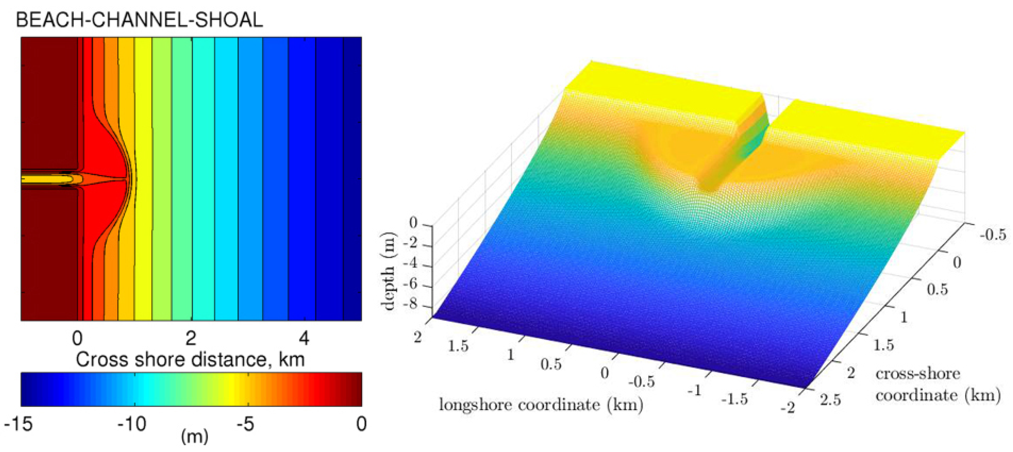
The inlet configuration chosen for the simulations presented in our study has been reproduced in strict resemblance with the one conceived by Olabarrieta et al. [9] (left panel of Figure 3) for the analysis of wave-current interactions at a tidal inlet. The study by Olabarrieta et al. (OL14 hereinafter) aimed at assessing the physical processes involved in the interaction between currents, gravity waves, and bathymetry at inlets. We here use the same configuration for three main scopes: (i) to assess the validity of the river mouth modelling described in the previous section; (ii) to illustrate how macrovortices are generated by differential breaking at the mouth and shoal edges; (iii) to perform a parametric analysis of the role of sub-grid turbulence and seabed friction on the evolution and dissipation of the macrovortices. The results of these analyses are reported, in the same sequence, in the next section.

The inlet area is characterized by a main channel about 300 m wide and 5 m deep at the central axis, which opens to a semicircular, symmetric ebb shoal zone of minimum depth 2 m, extending 1 km offshore of the inlet mouth. The main channel also crosses the shoal and connects the inlet to the offshore area. The beach exhibits a Dean equilibrium profile given by the expression $d=A{x}^{\frac{2}{3}}$, where d is the water depth, x is the cross-shore distance, measured offshore from the mouth, and the profile scale factor A is set equal to $0.05$ in agreement with the numerical setup by OL14. The computational domain generated for our simulations is 3 km long in the cross-shore direction and 4 km long in the alongshore direction, and has been discretized into a computational mesh with node spacings $\mathsf{\Delta }x=10$ m and $\mathsf{\Delta }y=25$ m in the x and y direction respectively. The resulting mesh can be seen in the right panel of Figure 3 and allows to describe the chosen waves (see below) with at least 15 nodes per wavelength.

The bed roughness $k_s$ for the evaluation of the Chezy seabed friction coefficient $c_{\tau }$ (see (5)) is set equal to $2\times {10}^{-4}\mathrm{m}$, in agreement with OL14. For all tests, the increase in apparent bed roughness and friction coefficient due to waves has not been considered.

To evaluate the capability of the solver to reproduce the hydrodynamics typical of a river mouth aim (i) above, benchmarking tests have been performed beforehand and a comparison with the results of the study by OL14 has been made. Our NSWE solver is depth-averaged and wave-resolving; OL14, conversely, applied the wave-averaged COAWST solver [48] for their numerical simulations. The data set used for the benchmarking coincides with that used by OL14 for their wave-current interaction tests in condition of strong outflow, and differs from that used for the analyses aimed at scopes (ii) and (iii) of above. In particular, for the benchmark tests an outflowing current of 1.1 m/s has been opposed to three distinct wave conditions: no waves, a spectral wave of significant height $H_s=0.5$ m, and a spectral wave of significant height $H_s=1.5$ m. These two wave regimes have been generated by means of a JONSWAP spectrum with a peak period $T_p$ set to 10 s. In all our benchmarking tests a value of the eddy viscosity parameter $\lambda =0$ is used. The results of the benchmarking analysis are presented in Section 4.1.

Moreover, a simple sensitivity test has been executed to inspect the influence of the mesh size over the definition and evolution of the numerical solution, with specific focus on the vorticity which, being defined by velocity derivatives, is the variable most sensitive to mesh refinement. To this end, test TW1, with waves interacting with the river current and no dissipation mechanism activated, has been performed with two different mesh resolutions. In addition to the “reference” mesh size (10 m × 25 m), a mesh with tighter node spacings $\mathsf{\Delta }x=7.5$ m and $\mathsf{\Delta }y=15$ m in the x and y direction have been chosen for the new test TW1.M2. The results of such comparison are given in Section 4.2.1.

To assess the role of waves, frictional and viscous dissipative forces on the global hydrodynamics and vorticity patterns, a parametric analysis with different wave conditions, bed friction coefficient $c_{\tau }$, and eddy viscosity parameter $\lambda$ has been performed. Two wave conditions have been used: no waves, and a representative monochromatic sinusoidal wave of height $1.5$ m and period 15 s. As for frictional effects, some tests have been undertaken disregarding the seabed friction, whereas others include a friction coefficient $c_{\tau }$ evaluated according to Equation (5). Finally, the tests used to assess the role of sub-grid turbulence have been run using a calibration parameter $\lambda =0.1$. This value has been chosen in agreement with the eddy viscosity model (9), to match the average real-case field conditions and obtain an average horizontal eddy viscosity in the order of 1 m²/s over the shoal zone, where the water depth is (2–3) m. A value of 1 m²/s has been also used for the tests in OL14, based on [49].

In all tests, a current of speed 1.1 m/s flowing out of the river mouth is used. This value corresponds to the current velocity for the tests with strong outflow conditions proposed in the work by OL14.

Table 1. Summary of the performed numerical tests.

Test	Current	Wave	Wave Direction	Friction	Viscosity	Mesh
TC1	1.1 m/s	—	—	—	—	10 m × 25 m
TC2	1.1 m/s	—	—	$k_s=2\times {10}^{-4}$	—	10 m × 25 m
TC3	1.1 m/s	—	—	—	$\lambda =0.1$	10 m × 25 m
TC4	1.1 m/s	—	—	$k_s=2\times {10}^{-4}$	$\lambda =0.1$	10 m × 25 m
TW1	1.1 m/s	$H=1.5$ m; $T=15$ s	0°	—	—	10 m × 25 m
TW2	1.1 m/s	$H=1.5$ m; $T=15$ s	0°	$k_s=2\times {10}^{-4}$	—	10 m × 25 m
TW3	1.1 m/s	$H=1.5$ m; $T=15$ s	0°	—	$\lambda =0.1$	10 m × 25 m
TW4	1.1 m/s	$H=1.5$ m; $T=15$ s	0°	$k_s=2\times {10}^{-4}$	$\lambda =0.1$	10 m × 25 m
TW1.1	1.1 m/s	$H=1.5$ m; $T=15$ s	0°	—	—	10 m × 25 m
TW1.2	1.1 m/s	$H=1.5$ m; $T=15$ s	10°	—	—	10 m × 25 m
TW1.3	1.1 m/s	$H=1.5$ m; $T=15$ s	20°	—	—	10 m × 25 m
TW1.4	1.1 m/s	$H=1.5$ m; $T=15$ s	30°	—	—	10 m × 25 m
TW4.1	1.1 m/s	$H=1.5$ m; $T=15$ s	0°	$k_s=2\times {10}^{-4}$	$\lambda =0.1$	10 m × 25 m
TW4.2	1.1 m/s	$H=1.5$ m; $T=15$ s	0°	$k_s={10}^{-3}$	$\lambda =0.1$	10 m × 25 m
TW4.3	1.1 m/s	$H=1.5$ m; $T=15$ s	0°	$k_s=2\times {10}^{-4}$	$\lambda =0.5$	10 m × 25 m
TW4.4	1.1 m/s	$H=1.5$ m; $T=15$ s	0°	$k_s={10}^{-3}$	$\lambda =0.5$	10 m × 25 m
TW1.M1	1.1 m/s	$H=1.5$ m; $T=15$ s	0°	—	—	10 m × 25 m
TW1.M2	1.1 m/s	$H=1.5$ m; $T=15$ s	0°	—	—	7.5 m × 15 m

shows a summary of the tests made for the parametric analysis and the dissipative contributions (friction, viscosity, both, or none) activated in each of them; the results are presented in Section 4.2.2 and Section 4.2.3. All simulations have been run for a time long enough to achieve some sort of steady state in terms of rotational flow energy.

To better inspect the possible changes of vorticity patterns with wave direction, test TW1 (featuring interacting current and waves, with neither friction nor viscosity dissipation; see Table 1) has been repeated four times, with four different angles of wave approach: 0°, 10°, 20°, and 30°, respectively. The resulting vorticity maps are presented and discussed in Section 4.2.4.

To evaluate the effect of the magnitude of friction and sub-grid turbulence dissipation mechanisms into the development of vortical patterns, test TW4 (waves interacting with current, both friction and viscosity dissipation activated) has been repeated four times. In each test the intensity of frictional effects and viscous dissipation have been altered, respectively by changing the bed roughness $k_s$ and the viscosity calibration parameter $\lambda$, giving rise to four different combinations of friction and viscosity. The results of this analysis is given in Section 4.2.5.

Finally, we propose some simple considerations on the global amount of large-scale vorticity present in the basins. To do this, use is made of the Okubo-Weiss (OW) parameter for 2-dimensional vortical flows [50,51] which is defined as follows:

$$OW=s_n^2+s_s^2-{\omega }^2,$$

(31)

where $s_n$ and $s_s$ are the normal and shear components of strain, respectively, and $\omega$ is the vorticity for 2-dimensional flows:

$$s_n=\frac{\partial u}{\partial x}-\frac{\partial v}{\partial y},s_s=\frac{\partial v}{\partial x}+\frac{\partial u}{\partial y}\mathrm{and}\omega =\frac{\partial v}{\partial x}-\frac{\partial u}{\partial y}.$$

(32)

According to the OW criterion the vortical flow can be roughly divided into two types of regions. Where $OW>0$, $s_n^2+s_s^2>{\omega }^2$ and the flow is dominated by fluid straining more than vorticity. Conversely, where $OW<0$, $s_n^2+s_s^2<{\omega }^2$ and the rotational effects dominate over deformation, giving birth to vortices [23].

An integral Okubo-Weiss parameter ${\mathsf{\Psi }}_{xy}$, furthermore, is defined as follows:

$${\mathsf{\Psi }}_{xy}={\int }_y{\int }_{x}O{W}^{\prime }\mathrm{d}x\mathrm{d}y$$

(33)

where

$$O{W}^{\prime }=\left\{\begin{array}{c}OW\mathrm{when}OW\le 0,\hfill \\ 0\mathrm{when}OW>0.\hfill \end{array}\right.$$

(34)

For each of the tests discussed in Section 4.2.1, Section 4.2.2, and Section 4.2.3, a numerical integration of only the negative OW over the computational domain is performed via application of the trapezoidal method. The obtained “integral OW parameter” (33) is, thus, used as a proxy to evaluate the overall amount of large-scale vortical energy in the flow, as a function of time. Small oscillations in the time series may indicate the organization and rapid dissipation of moderate-sized vortices, which account for only a modest increase of vortical energy over the whole domain. A steady and consistent increase in the time series over a time interval, conversely, is caused by the development of one or more macrovortices increasing their intensity and size.

4. Results and Discussion

From here onwards and whenever reasonable, the involved variables and figures are made dimensionless by setting the vertical length scale $d_0$ of Equations (12) equal to the still water depth at the offshore boundary of the domain, the horizontal length scale $L_0$ equal to the cross-shore extension of the shoal region from the channel mouth, and using the derived time scale $t_0=L_0/\sqrt{g{d}_0}$. In addition to the already defined dimensionless quantities (12), dimensionless forms for vorticity $\omega$ and the integral Okubo-Weiss parameter ${\mathsf{\Psi }}_{xy}$ (33) are as follows:

$$\tilde{\omega }=\omega t_0,{\tilde{\mathsf{\Psi }}}_{xy}={\mathsf{\Psi }}_{xy}\frac{t_0^2}{L_0^2}=\frac{{\mathsf{\Psi }}_{xy}}{g{d}_0}.$$

(35)

Some considerations on the magnitude of friction-based and viscosity-based dissipation are also proposed by means of the parameters $P_{\tau }$ and $P_{\lambda }$ (see Section 2.1.1), where the length scaling parameter $ϵ\approx {10}^{-3}$ over the shoal and $ϵ\approx {10}^{-2}$ offshore of the shoal, where depths are larger.

4.1. Evaluation of the Model for the River Mouth

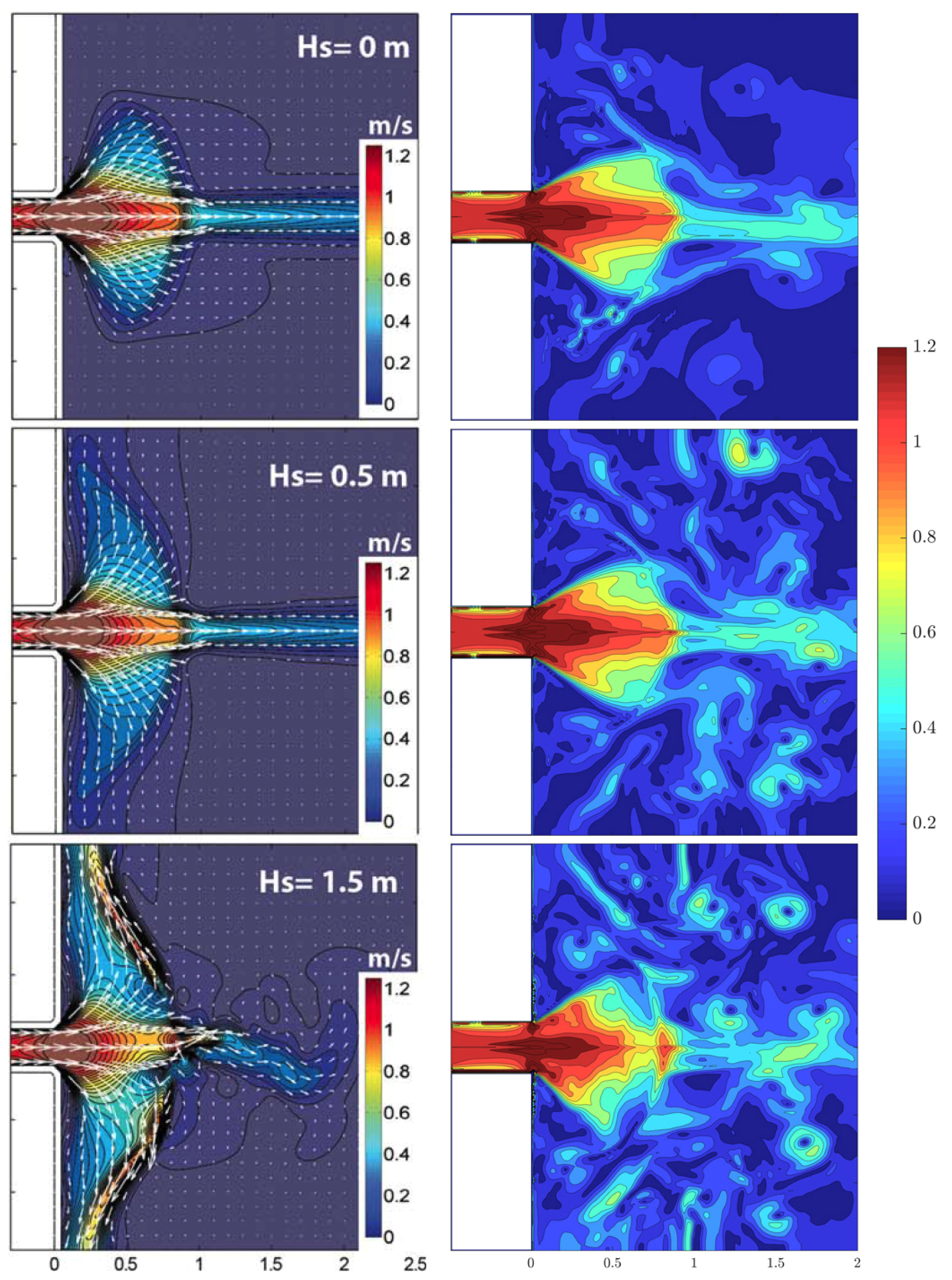
For the sake of evaluating the performance of our estuarine model, a comparison of velocity contour fields is presented in Figure 4, where the results of the tests of OL14 are shown in the left column, while the results from the corresponding benchmarking simulations, averaged over 100 s (10 wave periods), are shown in the right column.

Our depth-averaged, wave-resolving model manages to represent the main hydrodynamical features of the wave-current interaction displayed in the solution by OL14, such as the current speed increase at the mouth due to the gradual reduction of water depth, the jet current spreading over the shoal, and the seaward jet extension and thinning. The numerical tests by OL14 highlight a significant spreading of the river jet with medium-to-strong alongshore currents at the edge of the shoal (see middle and bottom left panels). On the other hand, our simulations show that the current jet undergoes a weaker longshore spreading and a significant generation of large-scale eddies (see middle and bottom right panels). Both differences suggest that our NSWE, wave-resolving solver produces a stronger breaking-induced dissipation of the incoming waves, which: (a) are less effective in pushing the river jet back to the coast and spread it in the alongshore, and (b) transfer, via differential breaking, a significant amount of energy to macrovortices.

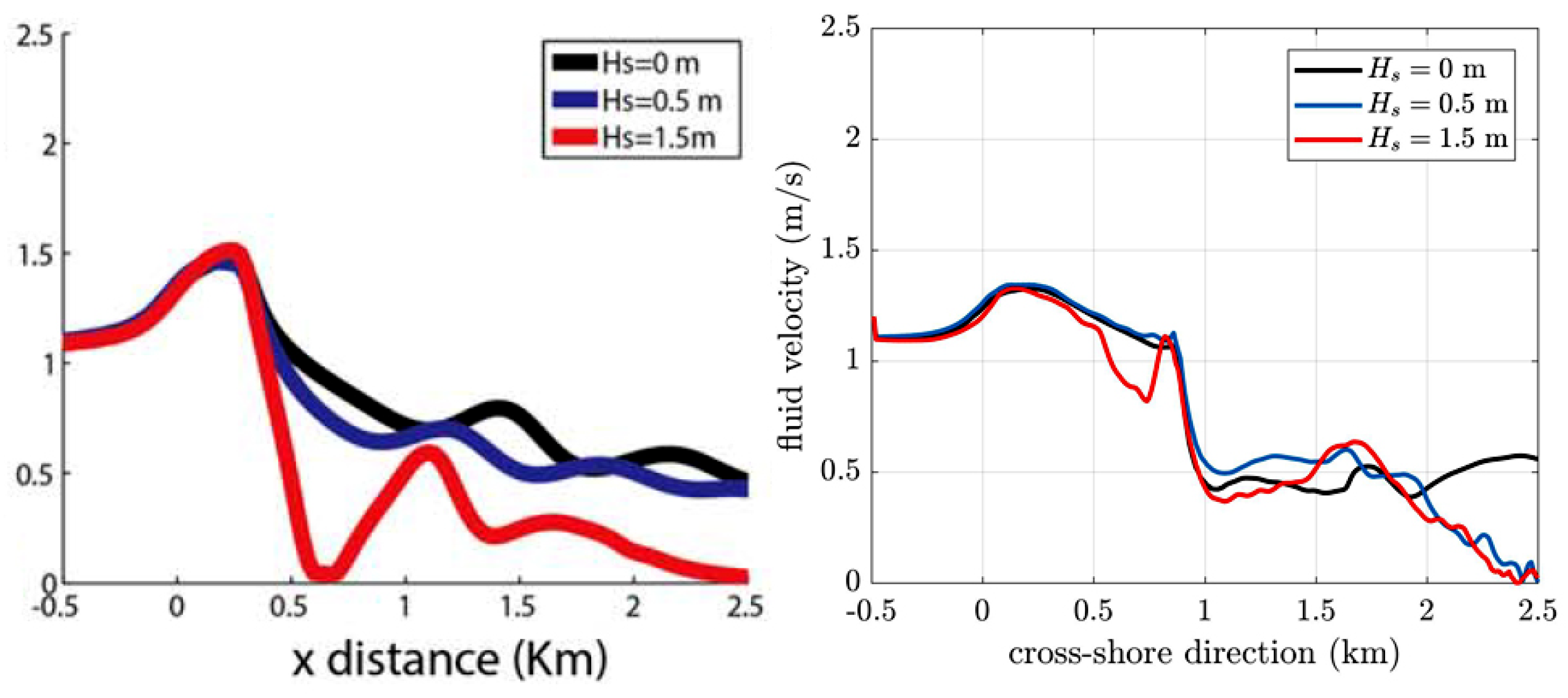
Figure 5 shows a comparison of the velocity computed along the main central axis. Results from the numerical simulations by OL14 are shown in the left panel, while the corresponding results from our benchmarking NSWE simulations are shown in the right panel. Both test campaigns show a similar global behavior, with the current gaining speed outside the mouth due to a gradual reduction of water depth and strong wave-breaking-induced undertow ($x\approx$ 0–0.3 km), then decreasing over the shoal mainly because of momentum loss and the action of bottom friction ($x\approx$ 0.2–0.9 km), and finally experiencing a decay at the transition between the ebb shoal and the beach profile. The latter decay, which is gentle except for the case with $H_s=1.5$ m in the test by OL14, is rather sharp in all NSWE simulations.

Notwithstanding some differences, mainly to be credited to the different nature of the two numerical solvers, our flow circulation model well represents the hydrodynamics of a simplified river mouth environment. Moreover, it also suggests a significant role of macrovortices in the energy redistribution of the wave-current interaction.

4.2. Vorticity Patterns and Global Vorticity

4.2.1. Sensitivity to Mesh Size

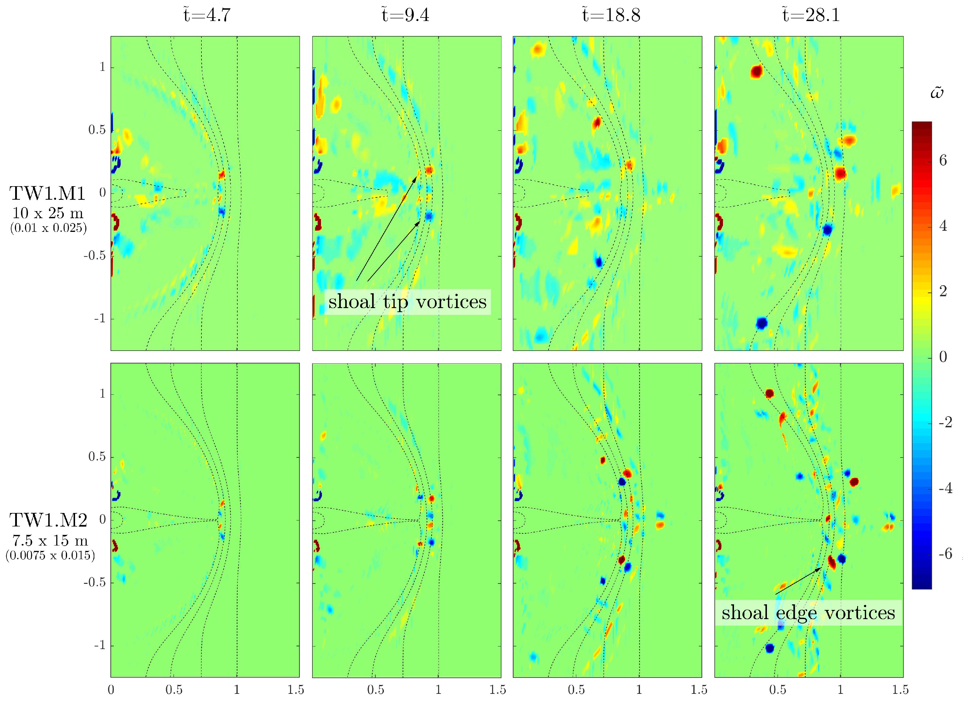
Figure 6 shows a preliminary comparison of vorticity maps for assessing the role of the mesh size on the simulated vorticity patterns that are thoroughly discussed in the next sections. Results from test TW1.M1, featuring a coarse mesh of 10 m × 25 m (0.01 × 0.025 in dimensionless units), are shown in the top panels. The bottom panels are relative to the test TW1.M2, performed with a finer mesh (7.5 m × 15 m, or 0.0075 × 0.015 in dimensionless units). Both tests feature a setup that corresponds to test TW1 (interacting waves and currents with no friction nor viscosity). The vorticity maps for the present tests, as well as for those in the next sections, have been extrapolated at four different time instants to show in a compact way the evolution of large-scale vortical structures.

The comparison reveals that vorticity generation patterns are qualitatively quite similar, with the bulk of vorticity injection focused along the border of the shoal in a symmetrical way. Well-formed macrovortices arise at the shoal tip, as a product of the interactions between breaking waves and outflowing currents, and gradually migrate outwards following the shoal curvature. In both tests mouth vortices, i.e., vortical structures developing at the corners of the channel mouth due to lateral spreading of the outflowing current, are absent. The increased spatial resolution in test TW1.M2, however, allows for more macrovortices to arise along the shoal edge; comparatively, test TW1.M1, which features a coarser mesh, presents wider zones of non-organized vorticity that has not yet rearranged into vortical structures. This is particularly visible in the inner parts of the shoal (top panels in Figure 6).

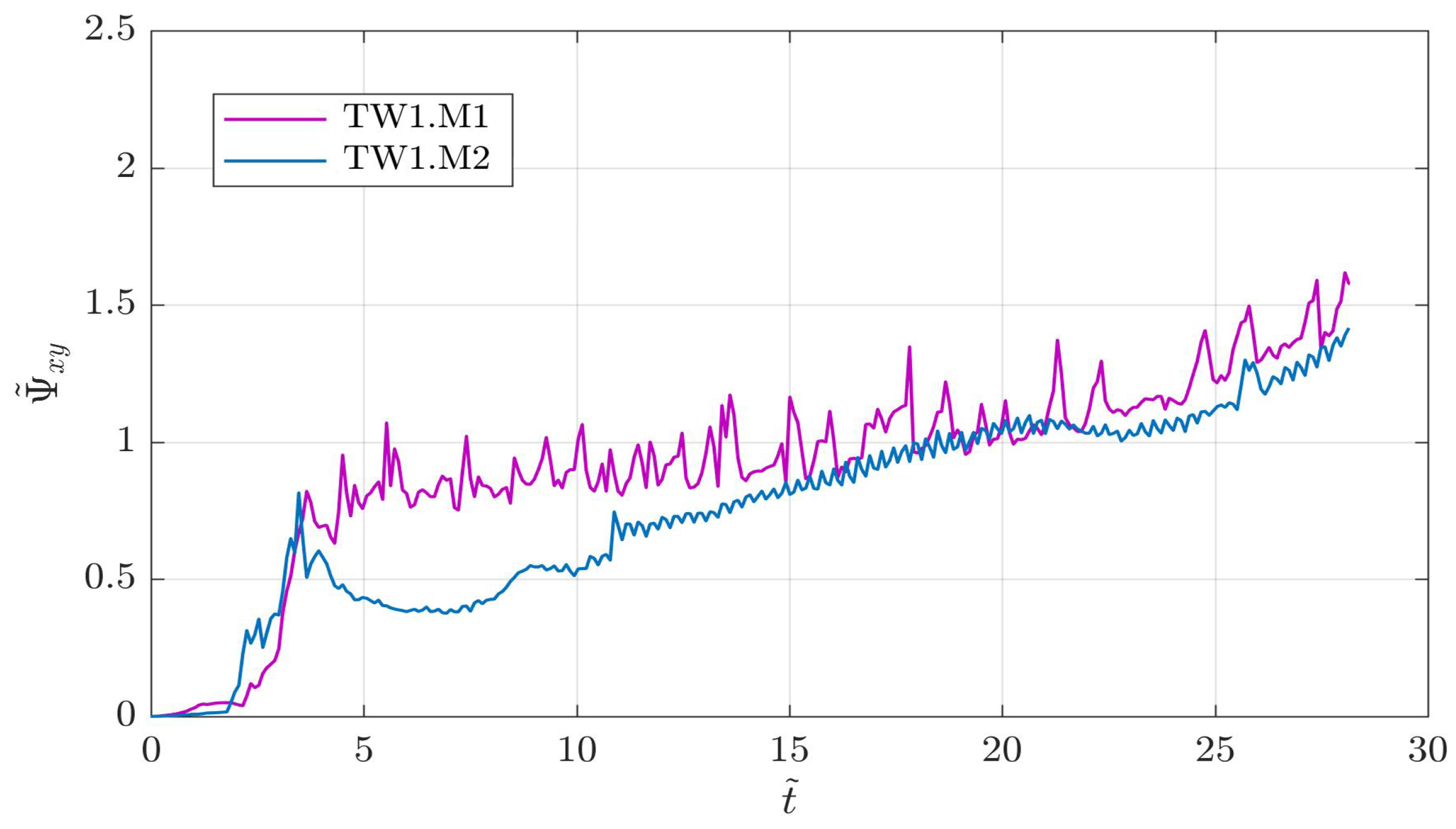
Figure 7 shows the time series of the (dimensionless) integral OW parameter ${\tilde{\mathsf{\Psi }}}_{xy}$ for preliminary tests TW1.M1 and TW1.M2.

Different mesh sizes inevitably have an impact on the numerical evaluation of vorticity, since the values of the space derivatives of velocities are different when different discretization lengths are assumed (see (32)). This presumably reflects into the different amplitudes and periods of the oscillations in ${\tilde{\mathsf{\Psi }}}_{xy}$. A discrepancy between the two time series can also be seen at the earlier times of the simulations, approximately at $\tilde{t}=4-11$. This is mainly due to the fine mesh test TW1.M2 giving less vorticity in the inner parts of the shoal than the coarse mesh test TW1.M1. Notwithstanding this, the similar values and long-term overall growth of ${\tilde{\mathsf{\Psi }}}_{xy}$ suggest that the amount of vortical energy injected into the basin by flow processes is roughly the same for both tests, regardless of the chosen mesh size.

4.2.2. Vorticity Patterns with No Waves

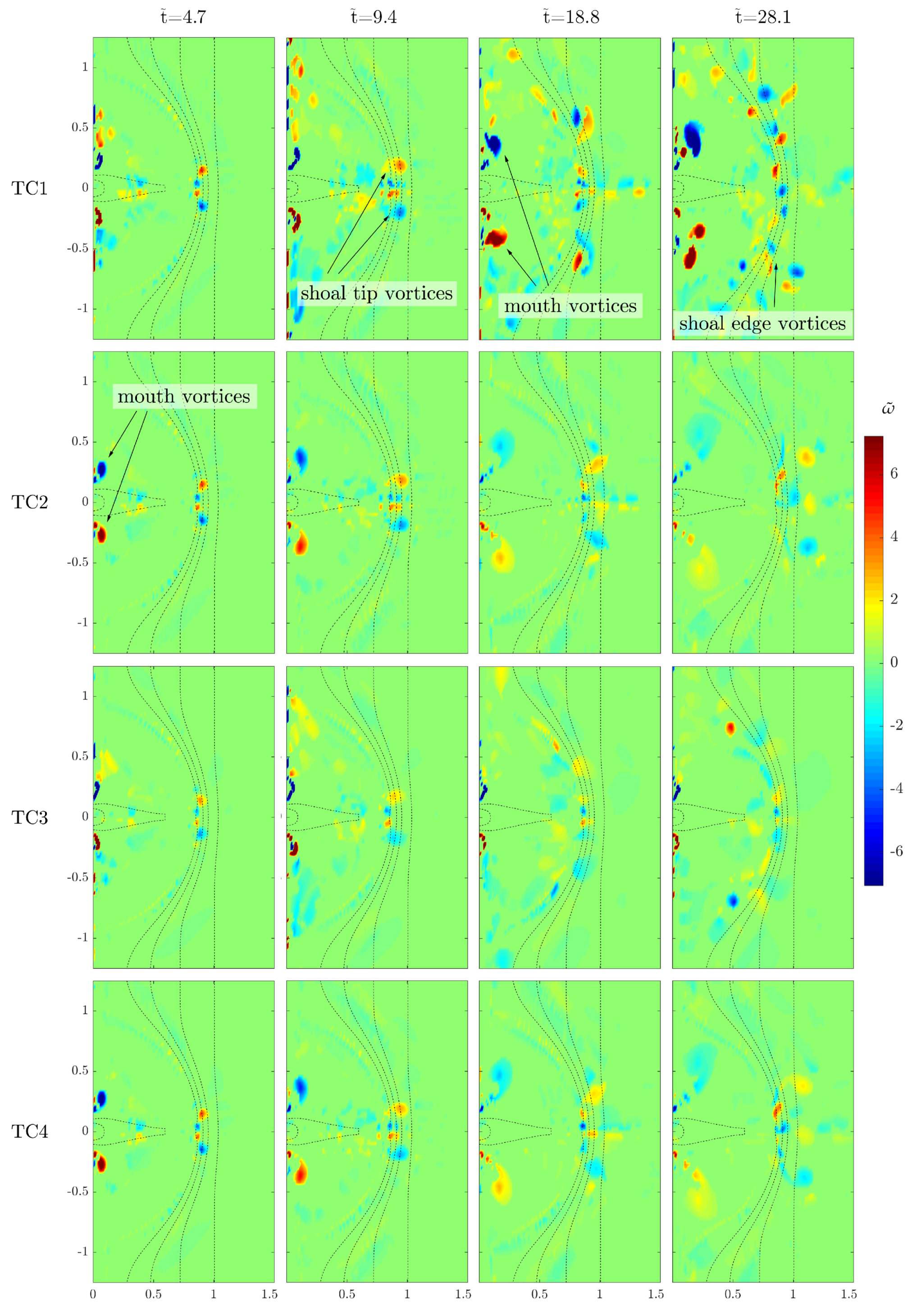
Figure 8 gives vorticity maps for the four numerical simulations carried out with only an outflowing current spreading over the shoal and no opposing waves. In each of these tests, labeled TC1 to TC4 (see Table 1), a unique combination of dissipative mechanisms has been activated, to better inspect the influence of both frictional and sub-grid turbulence effects.

All tests show a relevant generation of vorticity in two regions of the domain of interest: at the river mouth edges, where the river current exits the channel ($\tilde{x}\approx 0–0.1$), and at the shoal edge, where the shoal connects to the beach through a steep bottom gradient ($\tilde{x}\approx 1–1.2$). Although the global structure of the vortical flows originating at these regions is rather similar throughout the tests, the intensity and temporal evolution of vorticity, as well as its alongshore distribution to some extent, are highly dependent on the dissipation mechanisms at work.

In test TC1, the reference case (first row in Figure 8), no dissipation mechanism is active and a great amount of vorticity is seen near the river mouth since the earlier times of the simulation, due to the lateral spreading of the river current in the longshore direction. At later times ($\tilde{t}>10$) two intense macrovortices, approximately 100 m in diameter, develop in correspondence of the mouth corners and are gradually advected towards the inner parts of the shoal, as the current spreads (see the arrows in the third panel of the first row). Further, a pair of oppositely-signed macrovortices initially develops at the shoal tip ($\tilde{x}\approx 0.8–1$; see the arrows in the second panel of the first row), mainly due to lateral velocity gradients occurring at the boundaries between the main channel and the shoal plains, and are gradually advected laterally. Time passing, further turbulence develops along the boundary of the shoal (see the arrow in the fourth panel of the first row), organizes into vortices and grows unimpeded to values of about $\tilde{\omega }=4.5–5$ in absolute value, since the dissipative effects of both sub-grid turbulence and bed friction are neglected.

Since the bed friction coefficient is inversely proportional to the water depth (see Equations (4) and (5)), the contribution of seabed friction to the global dissipation of vorticity is expected to be more important in shallow waters, i.e., over the shoal and along the shoreline. This is confirmed in test TC2, where only the frictional dissipative effects are accounted for (second row in Figure 8). In fact, the mouth corner macrovortices generated at the start of the simulation are soon dissipated as their size increases and the wavenumber of the related turbulent motion decreases. The shoal tip macrovortices are also dissipated, albeit to a lesser extent, due to the effect of friction being less intense seaward of the shoal ($\tilde{x}>1$), where the water depth is larger. On the other hand, the vorticity at the shoal boundary, which is rather intense in test TC1, is absent here, indicating that the dissipative effect of seabed friction is noticeable also at the transition between the shoal and the beach, characterized by a steep bottom gradient.

For test TC3 (third row in Figure 8) the HLES routine described in Section 2.1 is activated, modeling the dissipation due to the sub-grid turbulence, while the seabed friction is neglected. The impact of the sub-grid turbulence dissipation on the vorticity patterns is evident at the most seaward parts of the shoal, where it is effective in limiting (although not suppressing altogether) the evolution and reorganization of macrovortices with respect to the reference case (test TC1). Sub-grid turbulence dissipation is effective also within the shoal, reducing size and intensity of the macrovortices at the river mouth corners. This is likely due to the considerable transversal velocity gradients occurring right outside of the mouth, where the rapidly spreading current interacts with the quiescent water on the shoal. This leads to large values of the velocity gradients in the inner shoal, which, in turn, induce an appreciable dissipation of flow energy and momentum (see Equations (10) and (11)).

Finally, for test TC4 (fourth row in Figure 8) both frictional effects and sub-grid turbulence contributions concur to dissipate the large-scale turbulence of the macrovortices. The vorticity patterns are similar to those of test TC2, where only friction-based dissipation is present: this suggests that, when both dissipation sources are present, large-scale dissipation by friction tends to dominate over the small-scale dissipation by sub-grid turbulence. Moreover, with respect to test TC2, the additional presence of sub-grid turbulence is effective in further restraining the formation of the shoal edge macrovortices.

4.2.3. Vorticity Patterns with Waves

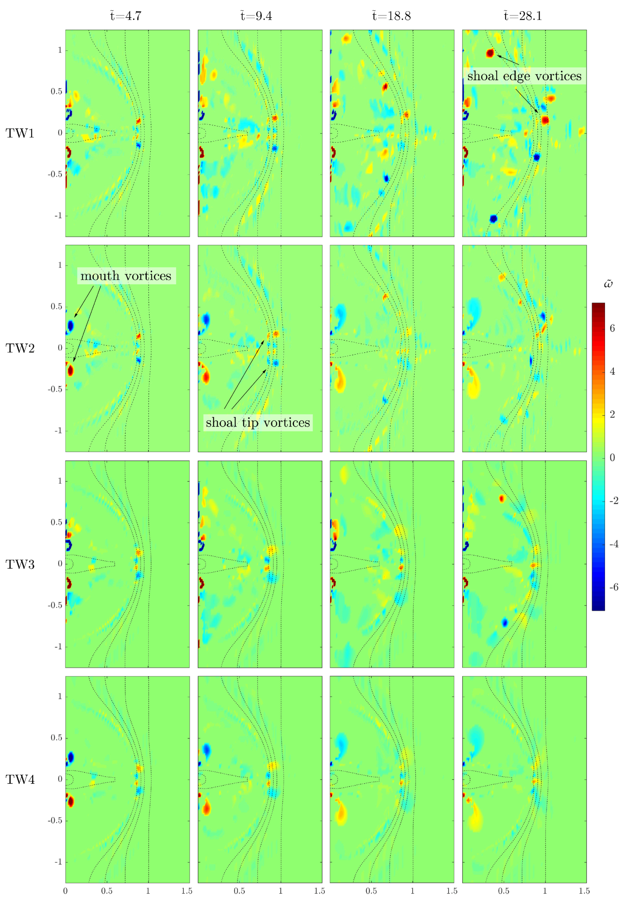
Figure 9 shows vorticity maps for the same test cases illustrated above, but for each simulation the river current is now opposed by a monochromatic sinusoidal wave. These tests are labelled TW1 to TW4 (see Table 1).

The dissipation-free test TW1 (first row in Figure 9) shows the presence of organized turbulence developing at the tip of the shoal, similarly to what occurs for test TC1. This may imply that in this zone the process of vortex generation is mainly dominated by current-related dynamics, with the effect of incoming waves being toned down in comparison. The maximum values for dimensionless vorticity in this test are around $\tilde{\omega }$ = 5.5–6 in absolute value. The vorticity structure of the wave-current interaction in this test is also characterized by a distinctive pattern which is roughly symmetrical with respect to the domain central axis. When waves are present, symmetrical vortices are formed, because of differential wave breaking, over the shoal edge and are advected diagonally towards the shore by the action of waves and interaction with the bathymetry, following the curvature of the shoal boundary itself. Such vortices are clearly visible in the last two panels of the first row in Figure 9. This behavior is in contrast to the essentially lateral advection experimented by the large eddies of test TC1 (see the last two panels in the first row in Figure 8). Vortex generation is mainly due to the previously cited depth-induced differential breaking experimented by the waves when they reach the shoal boundary. The portions of the wave fronts entering the shoal abruptly steepen and break because of the reduction of water depth, the steepening process being further enhanced by the effect of the opposing current. At the same time, the most lateral parts of the wave fronts are not yet broken since they are traveling over milder slopes. At the breaker lateral edges vorticity is injected into the flow and reorganizes into coherent vortices over time due to continuous and localized wave breaking. Once generated, these macrovortices migrate towards the shore in response to their interaction with the bathymetry, as illustrated by Brocchini and co-workers [10,11]. Furthermore, broken waves are also effective within the shoal, as they prevent the formation of the river mouth eddies.

For test TW2 (second row in Figure 9), only dissipation through bed friction is accounted for. The simulation notably shows the development of mouth vortices that are gradually dissipated, still being rather visible by the end of the test (last panel of the second row in Figure 9). The shoal boundary eddies are also similarly generated, albeit they are rapidly dampened as they travel inside the shoal due to friction.

Shoal boundary vortices are the main feature also in test TW3, in which only the sub-grid turbulence dissipation is active (third row in Figure 9). The small-scale turbulence dissipation of test TW3, however, is effective in reducing the size of the generated macrovortices when compared to the reference case TW1. Sub-grid viscosity-based turbulence has a greater effect when waves are present with respect to the no-wave condition (see test TC3), since waves generate strong, sign-changing velocity gradient in the alongshore direction that are continuous in time. This activates considerable and repeated dissipation by viscosity since such dissipation is dependent on the velocity gradients (see (10) and (11)).

Injection and reorganization of turbulence along the shoal boundary, as an effect of wave breaking, is also noticeable in test TW4 (fourth row in Figure 9), albeit the presence of both frictional and small-scale viscous dissipation strongly hinders the size and shoreward advection of generated macrovortices. Mouth vortices are very weak.

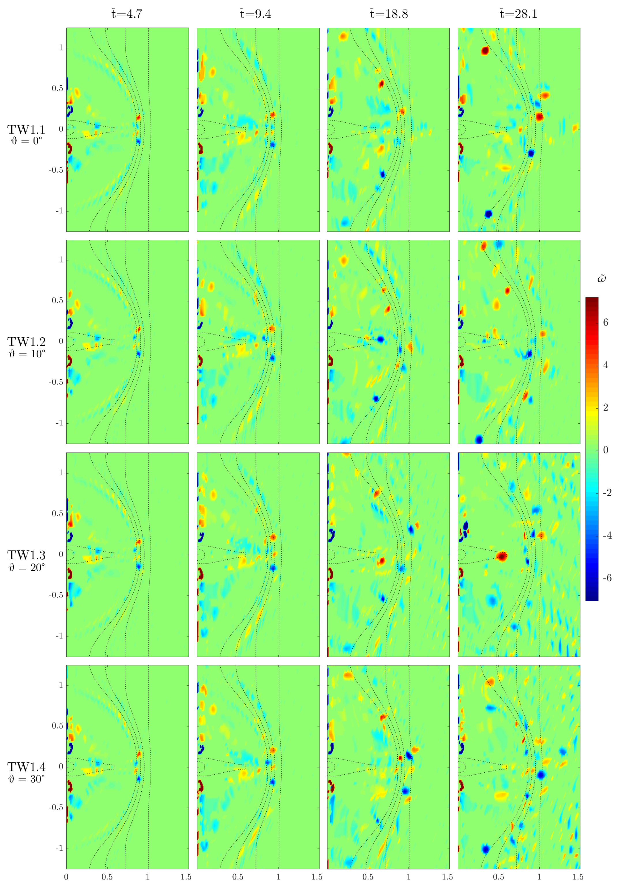
4.2.4. Vorticity Patterns as a Function of Wave Direction

Test TW1 (waves interacting with current, no friction nor viscosity dissipation; see top row in Figure 9) has been repeated four times with different directions of wave attack, in order to inspect the effect of wave direction on the vorticity patterns. Figure 10 shows vorticity maps for the four runs. From the top to the bottom row, the four angles of wave attack are 0°, 10°, 20°, and 30° with respect to the x-direction. In all panels the waves are approaching the shoreline from the bottom right angle. Test TW1.1, with a wave attack perpendicular to the seaward domain boundary, corresponds to test TW1 (see Section 4.2.3 and Figure 9); a slightly different notation for test names has been chosen for coherence in the nomenclature.

The performed tests reveal that different angles of wave approach do not break in a significant way the predominantly symmetrical pattern of vorticity already evidenced in the previous tests. This can be explained with the fact that the incoming waves surf through a considerable distance (more than 2 km) into the domain before hitting the shoal. As a side effect, wave fronts become more and more parallel to the shore thanks to well-known effects of refraction, and thus impact the shoal border at roughly the same angle, regardless of their direction upon entering the domain.

At earlier times in all tests ($\tilde{t}<10$), shoal tip vortices are formed at the same location than in tests TW (see Figure 9), suggesting that the wave direction is not a determinant variable in the birth and evolution of such vortices, which are, conversely, mainly dominated by the interaction between the outflowing current and the waves at the shoal border.

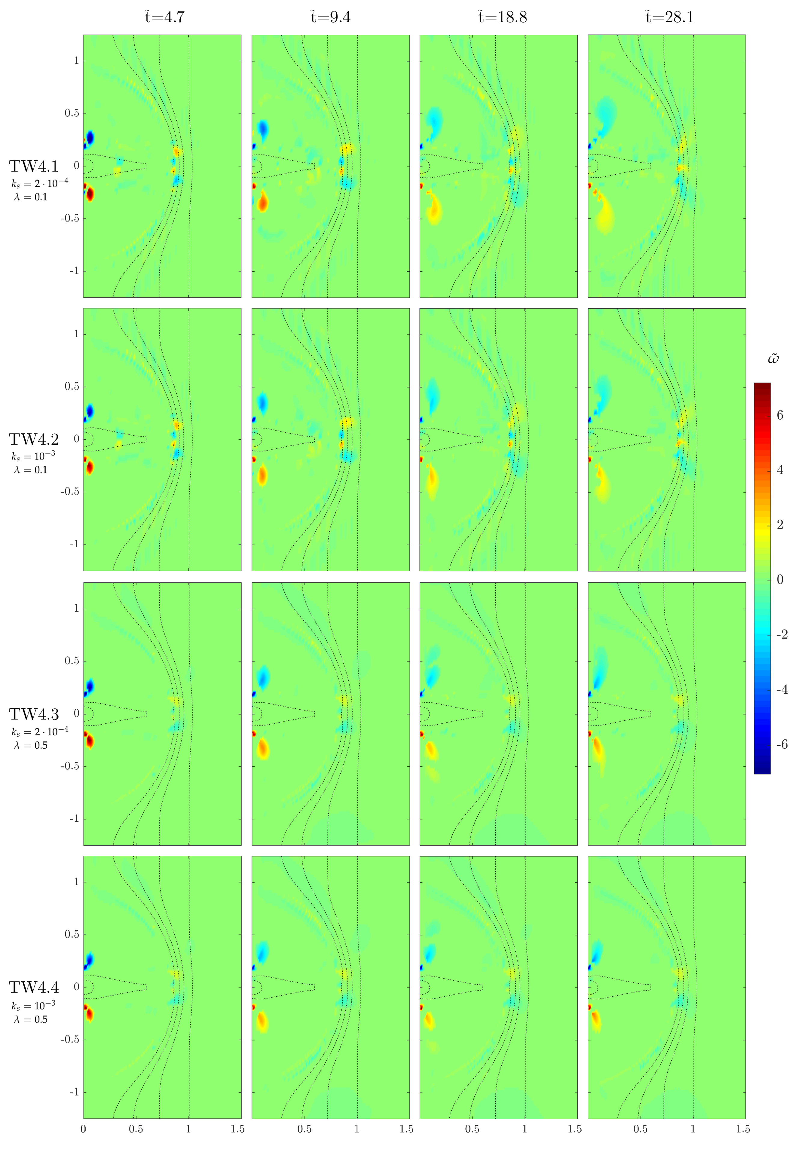
4.2.5. Sensitivity to Friction and Eddy Viscosity

To evaluate the effect of the magnitude of friction and sub-grid turbulence dissipation mechanisms into the development of turbulence, test TW4 has been repeated four times. In each test the intensity of frictional effects and viscous dissipation have been altered, respectively by changing the bed roughness $k_s$ and the eddy viscosity calibration parameter $\lambda$. Figure 11 shows the vorticity maps for the four iterations, labeled TW4.1 to TW4.4 (see also Table 1). Test TW4.1 corresponds to the reference test TW4 discussed in Section 4.2.3 and shown in the bottom row of Figure 9.

In test TW4.2 (second row in Figure 11) the action of dissipation due to friction is larger than in the reference case TW4.1, because of an increase in bed roughness $k_s$, while the sub-grid turbulence dissipation is unaltered. This leads to Chezy friction coefficients $c_{\tau }\approx {10}^{-3}$ and $P_{\tau }\approx 1$ over the shoal and near the numerical shoreline, while $P_{\tau }\approx {10}^{-1}$ off the shoal. The viscosity-related parameter is $P_{\lambda }\approx {10}^{-4}$ over the shoal, and $P_{\lambda }\approx {10}^{-3}$ outside the shoal. Therefore, frictional effects dominate over viscous dissipation. The increased effect of friction is visible through a slight reduction in the size and intensity of the mouth vortices. The extension of the region interested by mouth vorticity is reduced by frictional effects also during the phase of vortex dissipation (last two panels in the second row of Figure 11). The shoal tip vorticity, conversely, remains largely unaltered when increasing the friction; this suggests that, although the dissipative effect of friction is greater in magnitude than those of viscosity ($P_{\tau }={10}^{-1}>P_{\lambda }={10}^{-3}$ out of the shoal), the friction-based contribution only slightly affects the vortex morphology at the shoal tip and borders, similarly to the eddy viscosity contribution, mainly due to the increased water depths.

Test TW4.3 features an increase in the dissipative range of sub-grid turbulence with respect to the reference case. This is achieved by an increment of the eddy viscosity calibration parameter $\lambda$ from $0.1$ to $0.5$ (see Equation (9)). The size of frictional dissipation is unchanged. This leads to $P_{\lambda }\approx {10}^{-3}$ on the shoal and $P_{\lambda }\approx {10}^{-2}$ off the shoal; whereas $P_{\tau }\approx {10}^{-1}–1$ over the shoal and $P_{\tau }\approx {10}^{-2}–{10}^{-1}$ outside the shoal. In this test, friction still manages to exert a dominant role, especially in the shallow waters of the shoal, where the evolution of mouth vortices is dampened. However, the increase in viscosity dissipation has the notable consequence of reducing vorticity at the shoal tip and borders, while also causing a slight loss of coherence of the mouth vortices. All the above is confirmed by the vorticity maps shown in the third row in Figure 11. While exerting some effects also over the shoal, mainly through a reduction of the region of turbulence at the channel mouth, sub-grid turbulence has the greatest effects on the shoal tip vortices, which are strongly damped even during the earlier stages of the simulations ($\tilde{t}\le 10$; compare the first and third row of Figure 11).

Finally, in test TW4.4 (fourth row in Figure 11) both friction and sub-grid-turbulence dissipation are increased. $P_{\tau }\approx 1$ over the shoal and $P_{\tau }\approx {10}^{-1}$ outside the shoal; $P_{\lambda }\approx {10}^{-3}$ over the shoal and $P_{\lambda }\approx {10}^{-2}$ outside the shoal, with $P_{\lambda }$ increasing as the water depth grows. Therefore, friction is still dominant over viscosity at the shoal, while the balance becomes less skewed towards the shoal edge and offshore. The relative vorticity maps, thus, show a mix of the features described for tests TW4.2 and TW4.3: namely, a decrease of vortex intensity and size for mouth vortices (thanks to the enhanced friction-based dissipation), and a reduction of turbulence at the shoal tip (due to the enhanced viscosity-based dissipation).

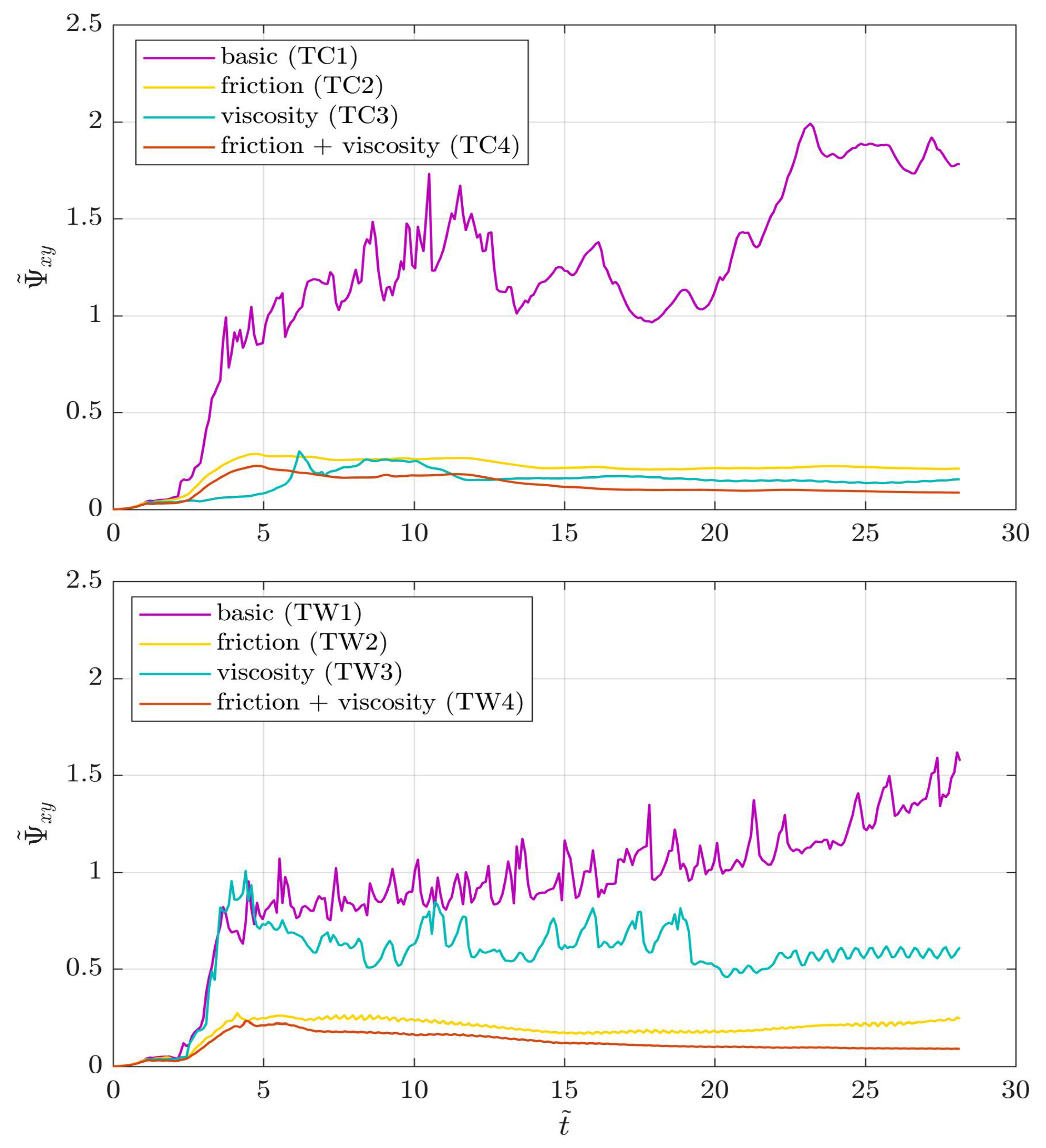
4.2.6. Global Vorticity for Currents and Waves Plus Currents

The time series of the integral dimensionless OW parameter ${\tilde{\mathsf{\Psi }}}_{xy}$ for the tests TC and TW, presented in Section 4.2.2 and Section 4.2.3, are illustrated in Figure 12. Note that the time series for test TW1 (purple line in the bottom panel) is the same as the purple line in Figure 7 (test TW1.M1).

The irregular behavior of the time series of ${\tilde{\mathsf{\Psi }}}_{xy}$ for the dissipation-free simulation with only river current (test TC1; purple line in the top panel) suggests that, when neither friction nor small-scale turbulence dissipation are accounted for, injection and dissipation of vorticity into the basin occur at a wide range of time scales. When waves are accounted for (test TW1; purple line in the bottom panel) the oscillations in ${\tilde{\mathsf{\Psi }}}_{xy}$ are more regular, with a clearly detectable rising trend ascribable to the continuous injection of vorticity promoted by breaking waves on the shoal boundary. The presence of waves into the domain, therefore, seems to have a regularizing effect on the evolution of turbulence.

The introduction of turbulence dissipation by seabed friction (tests TC2 and TW2; yellow lines) results in a friction magnitude parameter $P_{\tau }\approx {10}^{-1}–1$ (into the shoal) to ${10}^{-2}–{10}^{-1}$ (outside the shoal), whereas clearly $P_{\lambda }=0$ as viscosity-related dissipation is deactivated. Frictional dissipation results in a noticeable decrease of the overall amount of vortical energy for both test cases. The greater magnitude of $P_{\tau }$ on the shoal, moreover, implies that the dissipative action of seabed friction is stronger in that zone: this is also corroborated by the lower amount of vorticity in the shoal area given by tests TC2 and TW2 (second rows in Figure 8 and Figure 9) in comparison with the respective “reference” tests TC1 and TW1 (first rows in the same Figures). The strong influence of dissipation by friction is also apparent by inspection of the dimensionless OW parameter. ${\tilde{\mathsf{\Psi }}}_{xy}$ for the test with river current only (test TC2, top panel) is reduced by 75–80% in the earlier stages ($\tilde{t}<20$) mainly due to the consistent reduction in shoal vorticity, and by up to $90\%$ in the final stages ($\tilde{t}>20$) with respect to test TC1. For the test with interacting waves and currents (test TW2, bottom panel) the reduction in ${\tilde{\mathsf{\Psi }}}_{xy}$ with respect to test TW1 grows steadily in time, from $65\%$ at the beginning of the run, up to $85\%$ in the ending stages of the simulation. Furthermore, friction favours the emergence of a steady state for the global vorticity for both tests. This implies that the action of friction is competitive with the stirring of vorticity promoted by currents and waves, and the order of magnitude of both processes (stirring by waves/currents and dissipation by friction) is the same over the test duration.

The mechanism of turbulence dissipation through small-scale turbulence (tests TC3 and TW3; cyan lines) acts in different ways, according to the test case. For both tests, the viscosity-related magnitude parameter $P_{\lambda }\approx {10}^{-4}$ over the shoal and $P_{\lambda }\approx {10}^{-3}$ outside the shoal; $P_{\tau }=0$ since friction-based dissipation is deactivated. For the test with river current only (test TC3, top panel) sub-grid turbulence acts to a considerable decrease of global vortical energy, comparable to the reduction caused by frictional mechanisms. Albeit being smaller in magnitude with respect to the standard friction-based dissipation ($P_{\tau }\approx {10}^{-2}–1$ for tests TC2 and TW2), sub-grid turbulence dissipation mechanisms seem to be competitive in dissolving the vorticity injected by a river current only. On the other hand, when the current is opposed by waves (test TW3, bottom panel), the reduction in ${\tilde{\mathsf{\Psi }}}_{xy}$ is generally smaller (between $35\%$ and $65\%$ with respect to test TW1); this may suggest that the action of waves is effective in injecting a greater amount of vorticity, which is absent in the tests without waves. The action of viscosity, moreover, is greater outside of the shoal thanks to the greater depths, and leaves unorganized turbulence inside of the shoal. The regularization of the oscillations in ${\tilde{\mathsf{\Psi }}}_{xy}$, though, means a reduction and regularization of the time scale and intensity of vorticity stirring, especially towards the end of the simulation (the oscillations become more regular at $\tilde{t}>20$ for test TW3). In summary, in both tests small-scale turbulence manages to dissipate a variable amount of the vorticity generated during the initial stages of the runs and to keep the remaining vorticity roughly constant within the basin.

Finally, the combination of dissipation by seabed friction and sub-grid turbulence (orange lines) is the most effective in dissipating the overall vorticity, although the relative importance of the two factors for the dissipation process differs between the test cases and between each other ($P_{\tau }\approx {10}^{-2}–1$ and $P_{\lambda }\approx {10}^{-4}–{10}^{-3}$). Seabed friction and sub-grid dissipation are deemed to play a similar role when vorticity is stirred by the river current only (see the comparable reduction of ${\tilde{\mathsf{\Psi }}}_{xy}$ by both friction and viscosity in the top panel of Figure 12). On the other hand, the action of friction is enhanced with respect to viscosity-based dissipation, if turbulence is injected by the concurrent action of current and waves (see the far greater reduction of ${\tilde{\mathsf{\Psi }}}_{xy}$ induced by friction, with respect to the sub-grid-turbulence-induced, in the bottom panel of Figure 12).

5. Conclusions

Numerical simulations via a finite-volume numerical solver for shallow water flows have been exploited to achieve a better understanding of the dynamics of flow mixing and turbulence at an ideal river mouth configuration, as well as the role of bottom friction and sub-grid turbulence on the definition and temporal evolution of large coherent vortical structures. Flow dissipation by bed friction has been introduced through a simple Chezy-like approach. The effect of sub-grid vertical mixing has been accounted for through a suitable HLES formulation, in which the dissipative action of small-scale 3D turbulence is introduced through a global, depth-averaged eddy viscosity coefficient.

The performances of such wave-resolved model have been preliminarily tested against existing numerical simulations described in the work of Olabarrieta et al. [9], based on a wave-averaged solver. Both models are able to catch the main features of the wave-current interaction at a river mouth, albeit with some differences. The vertical-resolving model of OL14 seems to properly describe the alongshore currents observed in the field, but does not seem to give account of the potential vorticity generated at a river jet (e.g., see [52]). On the other hand, the wave-resolving NSWE model of Brocchini et al. [38] clearly reproduces macrovortices due to flow gradients caused by both the river jet and differential wave breaking, but predicts much weaker alongshore currents. This is in line with the strong wave breaking predicted by the NSWE model, which in turn leads to a considerable reduction of wave energy and generation of more intense macrovortices.

The analyses have identified two main regions of vorticity generation: at the inlet mouth due to current spreading, and along the shoal border as a consequence of the interaction between current, incoming waves, and bathymetry. In the definition and evolution of vorticity patterns, dissipation by means of friction seems to be generally dominant over sub-grid turbulence-based dissipation, especially over the shoal.

When only an outflowing river current is considered, dissipation through seabed friction is shown to be a strong agent in reducing the global amount of vorticity over the shoal and at the river mouth, where the mouth vortices are soon dissipated. At the shoal edge and further offshore seabed friction is not as effective, inducing only a mild reduction in vortex size and intensity. Conversely, dissipation through sub-grid turbulence has a greater effect at the shoal boundary, where the current slows down by feeling the increasing depth and develops negative velocity gradients, which are the fundamental contributions to viscosity-based dissipation.

When the interaction of current and waves is investigated, a significant amount of vorticity is generated, by differential wave braking, at the shoal edges and rolls up in the form of macrovortices. Wave breaking is also promoted by enhanced steepening thanks to the opposing current leaving the shoal. The shoal vortices are then advected towards the shore due to their interaction with the topography and the continuous action of waves. Again, seabed friction is shown to be the most important agent of regularization and dissipation of large-scale macrovortices within the shoal. Nonetheless, sub-grid turbulent motions also reduce the vorticity intensity at the shoal border, due to repeated velocity gradients. Waves are also effective in suppressing mouth vortices within the shoal.