Multi-Domain 2.5D Method for Multiple Water Level Hydrodynamics

Abstract

The mean water surface (interface) under the air cushion of a surface effect ship (SES) or an air cushion supported platform (ACSP) is generally lower than the outside water surface due to the overpressure of the air cushion. To precisely analyze the hydrodynamics under the air cushion, multiple water levels should be considered in numerical models. However, when using free surface Green’s functions as numerical methods, the water level difference cannot be taken into account, because free surface Green’s functions normally require users to set in the whole water domain a unique datum water surface that completely separates the air domain and the water domain. To overcome this difficulty, a multi-domain approach is incorporated into a 2.5D method that is based on a time domain free surface Green’s function with viscous dissipation effects in this paper. In the novel multi-domain 2.5D method, the water domain is partitioned into inner and outer domains, and the interface is located in the inner domain while the outside water surface is placed in the outer domain. In each domain there exists only one unique water level, while water levels in different domains are allowed to be different. Benefited from this characteristic, the multi-domain 2.5D method is able to precisely consider the water level difference and its influence on hydrodynamics. The newly proposed multi-domain 2.5D method is employed to predict the hydrodynamics of an SES, and it is confirmed that the multi-domain 2.5D method can give better numerical results than the single-domain one for the given case.

1. Introduction

In water-related engineering, there might exist multiple water surfaces with different levels, such as water separated by a dam or seawall, water flows passing through the channels of a M-craft, water under the air cushion of a surface effect ship (SES) or air cushion supported platform (ACSP), and so on. The water level difference could have an influence on the hydrodynamics of fixed or floating bodies in the water. For example, the pressurized air under an SES could reduce about 25% of the draught inside the cushion, whose impact should not be ignored.

There exist various numerical methods for solving the multiple water level hydrodynamics of an SES, e.g., Rankine source methods [1], finite element methods [2], unsteady Reynolds-averaged Navier-Stokes equation (URANS) methods [3], or even free surface Green’s functions [4,5,6]. Among these methods, the free surface Green’s functions are considered to be the most efficient due to the fact that source points are only distributed on the wetted surface rather than all water boundaries. In free surface Green’s functions, however, only a unique datum water surface can be defined in the flow field, and the water domain and air domain must be completely beneath and above this surface, respectively. The free surface condition for any water surface should be satisfied on the datum water surface. To meet this requirement, the datum surface is generally set on the highest water surface, i.e., water surface outside of the SES [6]. Obviously, this will cause the actual interface to be lower than the datum surface, which inevitably causes an adverse impact on predicting the hydrodynamics of the SES.

To overcome the abovementioned difficulties, a multi-domain concept, which divides the water domain into several domains and respectively solves the problem on each domain, is introduced into this paper. The multi-domain concept is used in fluid dynamics for several purposes. One is to realize the parallel computation technique [7,8,9], which decomposes the fluid domain into multiple regions, thus allowing calculations to be simultaneously performed in each region. Another purpose is to construct boundary conditions for shielded domains, which may be unknown in their original boundary value problems. To investigate waves passing through two vertical thin plates on the free surface, Shin and Cho [10] partitioned the fluid domain into three pieces using the two plates and their extension to the bottom, and respectively built up three boundary value problems (BVP) for three domains. Moreover, it was demonstrated that the multi-domain methods have better performance in predicting hydrodynamics. Chen and Duan [11] found that the multi-domain boundary element method (MD-BEM) is faster and more accurate in solving the hydrodynamics of a moonpool in comparison to the conventional BEM. Nonetheless, as far as we know, none of the existing multi-domain methods has been employed in tackling multiple water level problems.

In this paper, the multi-domain concept is first incorporated into the 2.5D (two and a half dimensional) method [12,13] based on the time domain free surface Green’s function with viscous dissipation effects [14] to form a multi-domain 2.5D method. The 2.5D method is a high-speed slender body method that could be able to predict the hydrodynamics of high-speed ships such as SES. The newly proposed method partitions the water domain into an inner domain and an outer domain, which contain, respectively, the interface and outside free surface. Thus, the interface could remain at its original position and the multi-domain 2.5D method would be able to precisely consider the multiple water levels and the influence of water level difference on hydrodynamics. The newly proposed multi-domain 2.5D method is validated by solving the hydrodynamics of an SES and comparing the numerical results with experimental ones.

2. Mathematical Models of the Multi-Domain 2.5D Method

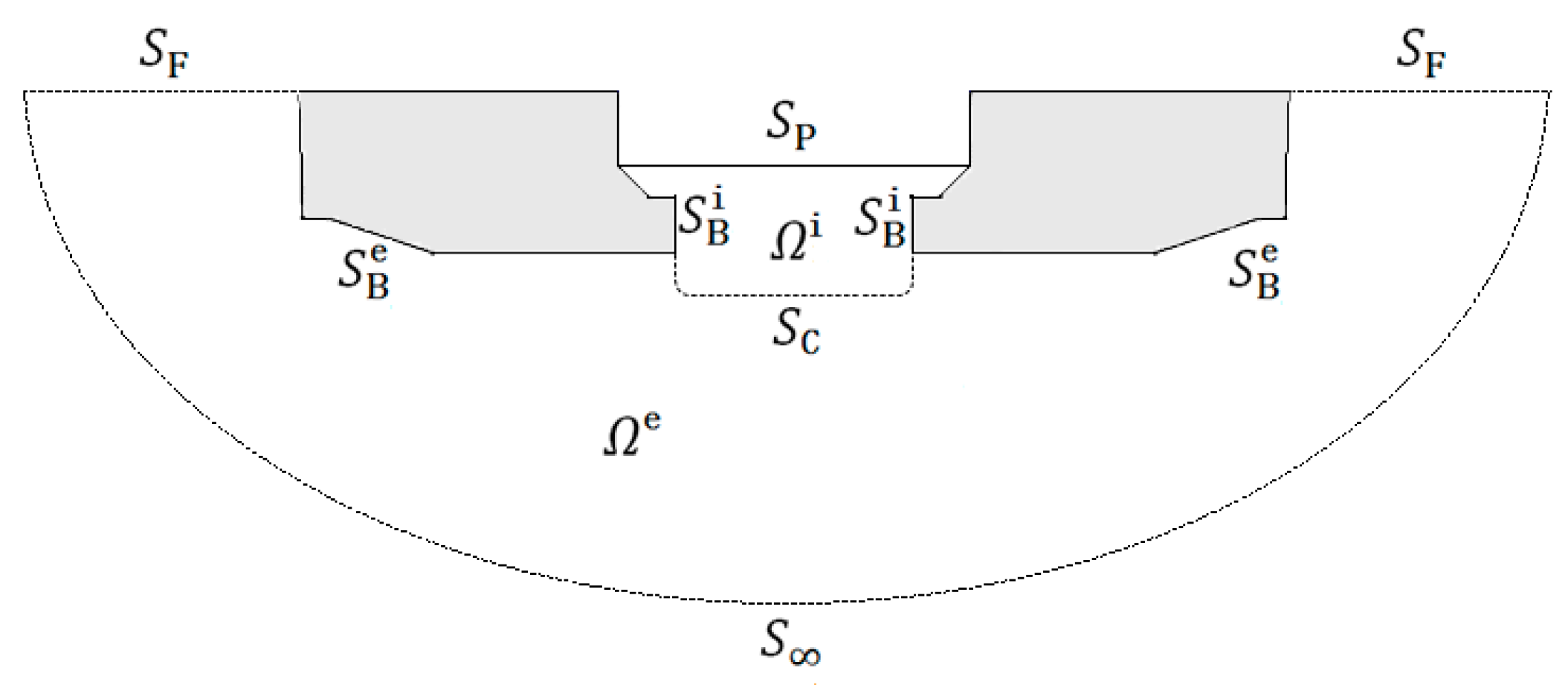
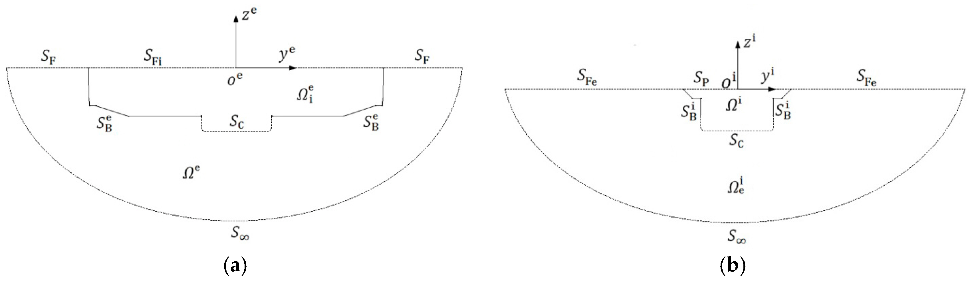
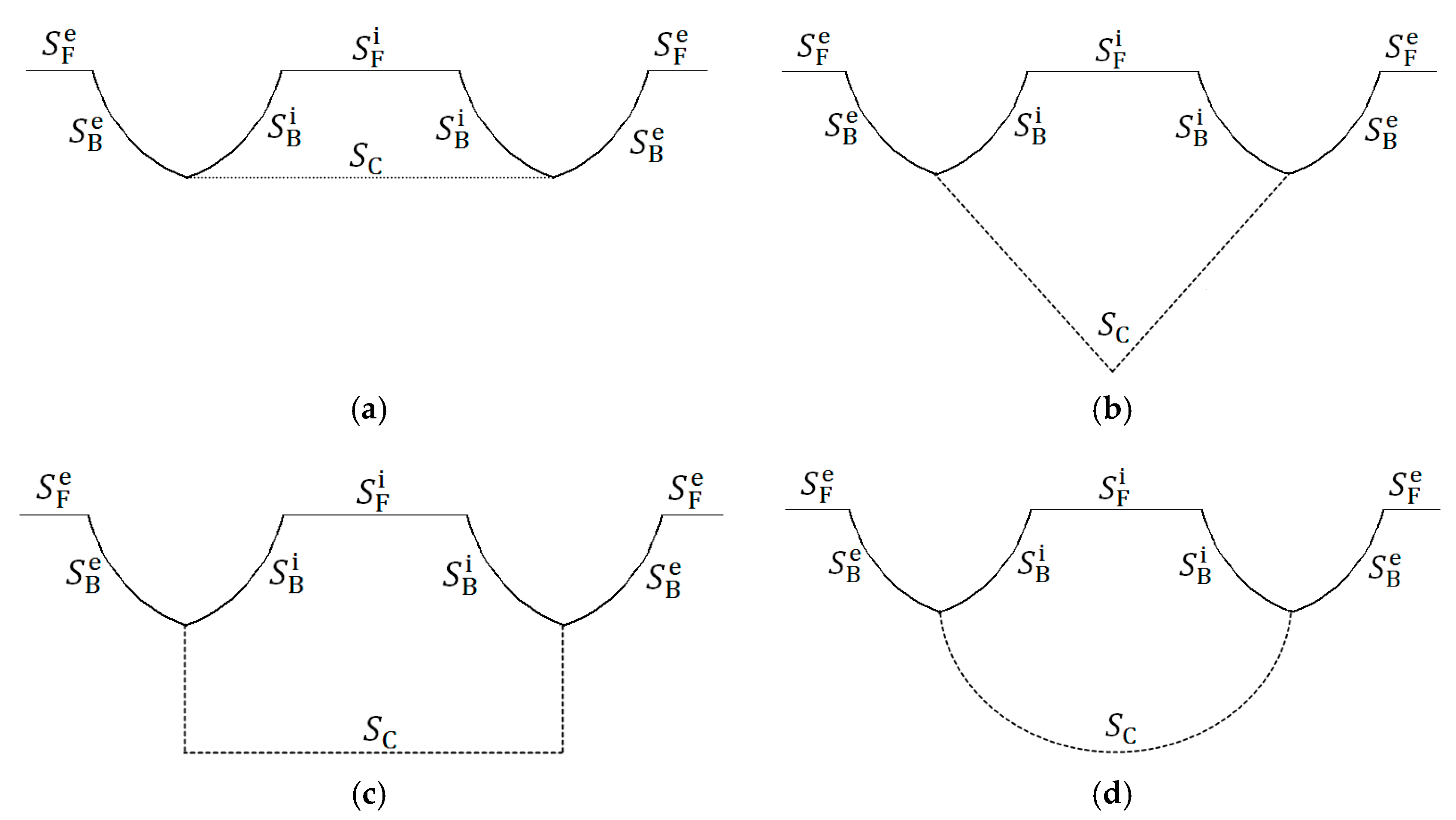
2.1. Partition of Water Domain and Boundary Value Problem

It is assumed that the water domain of an SES. $\Omega$ is enclosed by free surface $S_{\mathrm{F}}$, wetted surface $S_{\mathrm{B}}$, interface $S_{\mathrm{P}}$, and the boundary at infinite $S_{\infty }$. The fluctuating air cushion pressure on the interface of an SES can be expressed as:

$$\tilde{p}\left(x,y,t\right)=\widehat{p}\left(x,y\right){\mathrm{e}}^{\mathrm{i}\omega t}=-{\mathsf{\rho }}_{\mathrm{w}}{\mathrm{ge}}^{\mathrm{i}\omega t}{\displaystyle \sum }_{j=7}^{6+N_{\mathrm{P}}}{\eta }_j{n}_j\left(x,y\right)$$

(1)

where ${\mathsf{\rho }}_{\mathrm{w}}$ is the density of water, $\mathrm{g}$ is the gravity, $\omega$ is the pulsating frequency, ${\eta }_j$ is the equivalent waterhead of the fluctuating air pressure in the $j$-th mode, $N_{\mathrm{P}}$ is the number of modes, and $n_j\left(x,y\right)$ a complete set of orthogonal Fourier modes expanded on the interface defined as [15]:

$$n_j\left(x,y\right)=\left(\begin{array}{c}\cos \left(\alpha \mathsf{\pi }\left(x-x_{\mathrm{m}}\right)/l\right)\\ \sin \left(\alpha \mathsf{\pi }\left(x-x_{\mathrm{m}}\right)/l\right)\end{array}\right)\left(\begin{array}{c}\begin{array}{c}\cos \left(\beta \mathsf{\pi }y/b\right)\\ \sin \left(\beta \mathsf{\pi }y/b\right)\end{array}\end{array}\right)$$

(2)

where $\alpha ,\beta$ are 0 and even for the modes corresponding to the cosine or odd for the sine; and $l,b,x_{\mathrm{m}}$ are the length, breadth, and longitudinal center of the air cushion, respectively.

Within the framework of a linear high speed slender body assumption, the unsteady disturbance potential of water around the SES can be written as:

$${\varphi }_{\mathrm{T}}=\left\{{\eta }_0{\varphi }_0+{\displaystyle \sum }_{j=2}^6{\eta }_j{\varphi }_j+{\displaystyle \sum }_{j=7}^{6+N_{\mathrm{P}}}{\eta }_j{\varphi }_j\right\}{\mathrm{e}}^{\mathrm{i}\omega t}$$

(3)

where ${\eta }_0$ is the amplitude of the incident wave, ${\eta }_j\left(j=2,\dots ,6\right)$ the amplitude of the $j$-th motion mode, ${\varphi }_0$ the diffraction potential, ${\varphi }_j\left(j=2,\dots ,6\right)$ the radiation potential in the $j$-th motion mode, and ${\varphi }_j\left(j=7,\dots ,6+N_{\mathrm{P}}\right)$ the radiation potential in the $j$-th pressure mode.

The hydrodynamic BVP for the SES in water domain could be formulated as:

$$\{\begin{array}{ll}\frac{{\partial }^2{\varphi }_j}{\partial y^2}+\frac{{\partial }^2{\varphi }_j}{\partial z^2}=0,& \mathrm{in} \Omega \\ \left[{\left(\mathrm{i}\omega -U\frac{\partial }{\partial x}\right)}^2+\mathrm{g}\frac{\partial }{\partial z}\right]{\varphi }_j=\{\begin{array}{l}\mathrm{g}\left(\mathrm{i}\omega -U\frac{\partial }{\partial x}\right)n_j\left(x,y\right),\hfill \\ 0,\hfill \end{array}& \begin{array}{l}\mathrm{on} S_{\mathrm{P}},j=7,\dots ,6+N_{\mathrm{P}}\hfill \\ \mathrm{on} S_{\mathrm{F}}\cup \left(S_{\mathrm{P}},j=0,2,\dots ,6\right)\hfill \end{array}\\ \frac{\partial {\varphi }_j}{\partial n}=\{\begin{array}{ll}-\frac{\partial {\varphi }_{\mathrm{I}}}{\partial n},\hfill & j=0\hfill \\ \mathrm{i}\omega n_j+U{m}_j,\hfill & j=2,\dots ,6\hfill \\ 0,\hfill & j=7,\dots ,6+N_{\mathrm{P}}\hfill \end{array},& \mathrm{on} S_{\mathrm{B}}\\ {\varphi }_j=\nabla {\varphi }_j=0,& \mathrm{on} S_{\infty }\\ {\varphi }_j=\frac{\partial {\varphi }_j}{\partial x}=0,& \mathrm{at} x>x_{\mathrm{b}}\end{array}$$

(4)

where ${\varphi }_{\mathrm{I}}$ is the incident wave with unit amplitude; $U$ the advancing speed of the SES; $x_{\mathrm{b}}$ the $x$-axis of the bow; $n_j\left(j=1,\dots ,6\right)$ the generalized normal vector; $m_j$ is defined as $\left(m_1,m_2,m_3\right)=\left(0,0,0\right)$ and $\left(m_4,m_5,m_6\right)=\left(0,n_3,-n_2\right)$.

Normally, the interface $S_{\mathrm{P}}$ is lower than the free surface $S_{\mathrm{F}}$. To consider the water level difference between $S_{\mathrm{P}}$ and $S_{\mathrm{F}}$ using the 2.5D method, the water domain $\Omega$ is partitioned by the splitter $S_{\mathrm{C}}$ into the outer domain ${\Omega }^{\mathrm{e}}$ and the inner domain ${\Omega }^{\mathrm{i}}$ $\left(\Omega ={\Omega }^{\mathrm{i}}\cup {\Omega }^{\mathrm{e}}\right)$ (see Figure 1). As a result, the wetted surface $S_{\mathrm{B}}$ is divided into an outer wetted surface $S_{\mathrm{B}}^{\mathrm{e}}$ and an inner one $S_{\mathrm{B}}^{\mathrm{i}}$ $\left(S_{\mathrm{B}}=S_{\mathrm{B}}^{\mathrm{e}}\cup S_{\mathrm{B}}^{\mathrm{i}}\right)$. The free surface $S_{\mathrm{F}}$ and interface $S_{\mathrm{P}}$ are located in the outer domain ${\Omega }^{\mathrm{e}}$ and inner domain ${\Omega }^{\mathrm{i}}$, respectively. The splitter $S_{\mathrm{C}}$ could have any shape and is not limited to the one shown in Figure 1.

Let ${\varphi }_j^{\mathrm{e}}$ and ${\varphi }_j^{\mathrm{i}}$ be the water velocity potential in the outer domain ${\Omega }^{\mathrm{e}}$ and inner domain ${\Omega }^{\mathrm{i}}$, respectively. It is not difficult to obtain the BVP in the outer domain ${\Omega }^{\mathrm{e}}$:

$$\{\begin{array}{ll}\frac{{\partial }^2{\varphi }_j^{\mathrm{e}}}{\partial y^2}+\frac{{\partial }^2{\varphi }_j^{\mathrm{e}}}{\partial z^2}=0, & \mathrm{in} {\Omega }^{\mathrm{e}}\\ \left[{\left(\mathrm{i}\omega -U\frac{\partial }{\partial x}\right)}^2+\mathrm{g}\frac{\partial }{\partial z}\right]{\varphi }_j^{\mathrm{e}}=0,& \mathrm{on} S_{\mathrm{F}}\\ \frac{\partial {\varphi }_j^{\mathrm{e}}}{\partial n}=\{\begin{array}{ll}-\frac{\partial {\varphi }_{\mathrm{I}}^{\mathrm{e}}}{\partial n},\hfill & j=0\hfill \\ \mathrm{i}\omega n_j+U{m}_j,\hfill & j=2,\dots ,6\hfill \\ 0,\hfill & j=7,\dots ,6+N_{\mathrm{P}}\hfill \end{array},& \mathrm{on} S_{\mathrm{B}}^{\mathrm{e}}\\ {\varphi }_j^{\mathrm{e}}=\nabla {\varphi }_j^{\mathrm{e}}=0,& \mathrm{on} S_{\infty }\\ {\varphi }_j^{\mathrm{e}}=\frac{\partial {\varphi }_j^{\mathrm{e}}}{\partial x}=0,& \mathrm{at} x>x_{\mathrm{b}}\end{array}$$

(5)

where ${\varphi }_{\mathrm{I}}^{\mathrm{e}}$ is the incident wave in the outer domain.

Analogously, the BVP in the inner domain ${\Omega }^{\mathrm{i}}$ can be written as:

$$\{\begin{array}{ll}\frac{{\partial }^2{\varphi }_j^{\mathrm{i}}}{\partial y^2}+\frac{{\partial }^2{\varphi }_j^{\mathrm{i}}}{\partial z^2}=0, & \mathrm{in} {\Omega }^{\mathrm{i}}\\ \left[{\left(\mathrm{i}\omega -U\frac{\partial }{\partial x}\right)}^2+\mathrm{g}\frac{\partial }{\partial z}\right]{\varphi }_j^{\mathrm{i}}=\{\begin{array}{l}\mathrm{g}\left(\mathrm{i}\omega -U\frac{\partial }{\partial x}\right)n_j\left(x,y\right),\hfill \\ 0,\hfill \end{array}& \begin{array}{l}\mathrm{on} S_{\mathrm{P}},j=7,\dots ,6+N_{\mathrm{P}}\hfill \\ \mathrm{on} S_{\mathrm{P}},j=0,2,\dots ,6\hfill \end{array}\\ \frac{\partial {\varphi }_j^{\mathrm{i}}}{\partial n}=\{\begin{array}{ll}-\frac{\partial {\varphi }_{\mathrm{I}}^{\mathrm{i}}}{\partial n},\hfill & j=0\hfill \\ \mathrm{i}\omega n_j+U{m}_j,\hfill & j=2,\dots ,6\hfill \\ 0,\hfill & j=7,\dots ,6+N_{\mathrm{P}}\hfill \end{array},& \mathrm{on} S_{\mathrm{B}}^{\mathrm{i}}\\ {\varphi }_j^{\mathrm{i}}=\frac{\partial {\varphi }_j^{\mathrm{i}}}{\partial x}=0,& \mathrm{at} x>x_{\mathrm{b}}\end{array}$$

(6)

where ${\varphi }_{\mathrm{I}}^{\mathrm{i}}$ is the incident wave in the inner domain.

In addition, the velocity potentials ${\varphi }_j^{\mathrm{e}},{\varphi }_j^{\mathrm{i}}$ and their derivatives should be the same on the splitter $S_{\mathrm{C}}$:

$$\{\begin{array}{ll}\begin{array}{l}{\varphi }_j^{\mathrm{e}}={\varphi }_j^{\mathrm{i}},\hfill \\ \frac{\partial {\varphi }_j^{\mathrm{e}}}{\partial n}=\frac{\partial {\varphi }_j^{\mathrm{i}}}{\partial n},\hfill \end{array}\hfill & \mathrm{on}{S}_{\mathrm{C}}\hfill \end{array}$$

(7)

One can easily verify that the combination of BVPs from Equations (5)–(7) yields the BVP given by Equation (4), i.e., the original BVP for the SES in the water domain $\Omega$ with multiple water levels is equivalent to a BVP in the outer domain ${\Omega }^{\mathrm{e}}$ and another one in the inner domain ${\Omega }^{\mathrm{i}}$, and each domain from ${\Omega }^{\mathrm{e}}$ and ${\Omega }^{\mathrm{i}}$ only contains a unique water level. Thereby, one can employ the free surface Green’s function method (2.5D method) to solve these two BVPs.

2.2. Multi-Domain 2.5D Method

If the 2.5D method is based on the source and dipole mixed distribution model, one only needs to formulate the boundary integral equations along boundaries of the domain ${\Omega }^{\mathrm{e}}$ or ${\Omega }^{\mathrm{i}}$. However, the pure source distribution model is preferred in the 2.5D method. Thus, the pure source distribution model is employed in this paper. To this end, the outer domain ${\Omega }^{\mathrm{e}}$ is artificially extended to the interior domain (denoted by ${\Omega }_{\mathrm{i}}^{\mathrm{e}}$) enclosed by the outer wetted surface $S_{\mathrm{B}}^{\mathrm{e}}$, splitter $S_{\mathrm{C}}$, and artificial free surface $S_{\mathrm{Fi}}$ (Figure 2a), while the inner domain ${\Omega }^{\mathrm{i}}$ is artificially extended to the exterior domain (denoted by ${\Omega }_{\mathrm{e}}^{\mathrm{i}}$) surrounded by the inner wetted surface $S_{\mathrm{B}}^{\mathrm{i}}$, splitter $S_{\mathrm{C}}$, artificial free surface $S_{\mathrm{Fe}}$, and boundary at infinity $S_{\infty }$ (Figure 2b). It is worth noting that artificial free surfaces $S_{\mathrm{Fi}}$ and $S_{\mathrm{Fe}}$ have the same water level as $S_{\mathrm{F}}$ and $S_{\mathrm{P}}$, respectively. This is a novel multi-domain approach, which is different from the multi-domain approaches without domain extension adopted in the literature, such as in Reference [11].

Since the free surface conditions are only satisfied on the datum water level $z=0$, one has to define two local coordinate systems for two domains. As shown in Figure 2a, an SES-accompanied inertial coordinate system $o^{\mathrm{e}}-x^{\mathrm{e}}{y}^{\mathrm{e}}{z}^{\mathrm{e}}$ is defined in the outer domain ${\Omega }^{\mathrm{e}}$, which moves with speed $U$. When the SES is located at its mean position, the $x^{\mathrm{e}}$-axis points upstream and the $z^{\mathrm{e}}$-axis points vertically upward through the center of gravity (COG) of the SES. The origin $o^{\mathrm{e}}$ is placed in the plan of the mean outside free surface $S_{\mathrm{F}}$. Analogously, in Figure 2b another SES-accompanied inertial coordinate system $o^{\mathrm{i}}-x^{\mathrm{i}}{y}^{\mathrm{i}}{z}^{\mathrm{i}}$ is defined in the inner domain ${\Omega }^{\mathrm{i}}$, which is almost the same as $o^{\mathrm{e}}-x^{\mathrm{e}}{y}^{\mathrm{e}}{z}^{\mathrm{e}}$, except that the origin $o^{\mathrm{i}}$ is located on the interface $S_{\mathrm{P}}$. For simplicity, the notations “$\mathrm{e},\mathrm{i}$” on the top right of coordinates are ignored in following texts if no ambiguity occurs. However, one should note that the variables in each domain are always defined in their own coordinate systems.

The main difference between the current multi-domain method and those used in the literature for other purposes is that, in the current method, multiple local coordinate systems should be respectively defined for each domain and quantities in each domain must be defined in their own coordinate system, while in other multi-domain methods, generally only one global coordinate system is defined and quantities in different domains are defined in the same coordinate system.

Before employing 2.5D methods to solve the potentials, variable substitutions should be performed:

$$\{\begin{array}{l}x\left(t\right)=x_{\mathrm{b}}-Ut\hfill \\ {\psi }_j\left(t,y,z\right)={\mathrm{e}}^{\mathrm{i}\omega t}{\varphi }_j\left(x\left(t\right),y,z\right)\hfill \\ {\Pi }_j\left(t,y\right)={\mathrm{e}}^{\mathrm{i}\omega t}{n}_j\left(x\left(t\right),y\right)\hfill \end{array}$$

(8)

Let ${\psi }_j^{\mathrm{e}},{\sigma }_j^{\mathrm{e}}$ be the time-domain potential and source density in the outer domain, and ${\psi }_j^{\mathrm{i}},{\sigma }_j^{\mathrm{i}}$ be those in the inner domain. All outer domain potentials ${\psi }_j^{\mathrm{e}}\left(j=0,2,3,\dots ,6+N_{\mathrm{P}}\right)$ and sidehulls related inner domain potentials ${\psi }_j^{\mathrm{i}}\left(j=0,2,3,\dots ,6\right)$ can be solved using the tranditional time-domain Green’s function method [13], while fluctuating air cushion pressure-related inner domain potentials ${\psi }_j^{\mathrm{i}}\left(j=7,\dots ,6+N_{\mathrm{P}}\right)$ are associated with the mixed BVP and should be solved using the method presented in Appendix A.

The boundary integral equations and source density equations $\left(j=0,2,3,\dots ,6+N_{\mathrm{P}}\right)$ in the outer domain are given as:

$$\{\begin{array}{ll}\begin{array}{c}2\mathsf{\pi }{\psi }_j^{\mathrm{e}}\left(t,\mathit{p}\right)+{{\displaystyle \int }}_{S_{\mathrm{B}}^{\mathrm{e}}+S_{\mathrm{C}}}\overline{G}{\sigma }_j^{\mathrm{e}}\left(t,\mathit{q}\right)\mathrm{d}{s}_q={{\displaystyle \int }}_0^t\mathrm{d}\tau {{\displaystyle \int }}_{S_{\mathrm{B}}^{\mathrm{e}}+S_{\mathrm{C}}}\tilde{G}{\sigma }_j^{\mathrm{e}}\left(\tau ,\mathit{q}\right)\mathrm{d}{s}_q,\end{array}& \mathit{p}\in S_{\mathrm{B}}^{\mathrm{e}}\cup S_{\mathrm{C}}\\ \begin{array}{c}{{\displaystyle \int }}_{S_{\mathrm{B}}^{\mathrm{e}}+S_{\mathrm{C}}}{\sigma }_j^{\mathrm{e}}\left(t,\mathit{q}\right)\frac{\partial \overline{G}}{\partial n_p^{\mathrm{e}}}\mathrm{d}{s}_q-\mathsf{\pi }{\sigma }_j^{\mathrm{e}}\left(t,\mathit{p}\right)=-2\mathsf{\pi }\frac{\partial {\psi }_j^{\mathrm{e}}\left(t,\mathit{p}\right)}{\partial n_p^{\mathrm{e}}}+\\ {{\displaystyle \int }}_0^{t}d\tau {{\displaystyle \int }}_{S_{\mathrm{B}}^{\mathrm{e}}+S_{\mathrm{C}}}\frac{\partial \tilde{G}}{\partial n_p^e}{\sigma }_j^{\mathrm{e}}\left(\tau ,\mathit{q}\right)\mathrm{d}{s}_q,\end{array}& \mathit{p}\in S_{\mathrm{B}}^{\mathrm{e}}\\ \begin{array}{c}2\mathsf{\pi }\frac{\partial {\psi }_j^{\mathrm{e}}\left(t,\mathit{p}\right)}{\partial n_p^{\mathrm{e}}}+{{\displaystyle \int }}_{S_{\mathrm{B}}^{\mathrm{e}}+S_{\mathrm{C}}}{\sigma }_j^{\mathrm{e}}\left(t,\mathit{q}\right)\frac{\partial \overline{G}}{\partial n_p^{\mathrm{e}}}\mathrm{d}{s}_q-\mathsf{\pi }{\sigma }_j^{\mathrm{e}}\left(t,\mathit{p}\right)=\\ {{\displaystyle \int }}_0^t\mathrm{d}\tau {{\displaystyle \int }}_{S_{\mathrm{B}}^{\mathrm{e}}+S_{\mathrm{C}}}\frac{\partial \tilde{G}}{\partial n_p^{\mathrm{e}}}{\sigma }_j^{\mathrm{e}}\left(\tau ,\mathit{q}\right)\mathrm{d}{s}_q,\end{array}& \mathit{p}\in S_{\mathrm{C}}\end{array}$$

(9)

where $\mathit{p},\mathit{q},\overline{\mathit{q}}$ are the field point, source point, and mirror of the source point on the mean free surface, respectively; $r_{pq},r_{p\overline{q}}$ are the distance between $\mathit{p}$ and $\mathit{q}$, $\mathit{p}$ and $\overline{\mathit{q}}$, respectively.

On the other hand, the equations in the inner domain are given as:

$$\{\begin{array}{ll}\begin{array}{c}2\mathsf{\pi }{\psi }_j^{\mathrm{i}}\left(t,\mathit{p}\right)+{{\displaystyle \int }}_{S_{\mathrm{B}}^{\mathrm{i}}+S_{\mathrm{C}}}\overline{G}{\sigma }_j^{\mathrm{i}}\left(t,\mathit{q}\right)\mathrm{d}{s}_q={{\displaystyle \int }}_0^t\mathrm{d}\tau {{\displaystyle \int }}_{S_{\mathrm{B}}^{\mathrm{i}}+S_{\mathrm{C}}}\tilde{G}{\sigma }_j^{\mathrm{i}}\left(\tau ,\mathit{q}\right)\mathrm{d}{s}_q-\\ \begin{array}{c}{{\displaystyle \int }}_0^t\mathrm{d}\tau {{\displaystyle \int }}_{S_{\mathrm{P}}}{\Pi }_j\left(\tau ,\eta \right)\frac{\partial \tilde{G}}{\partial \tau }\mathrm{d}{s}_q,\end{array}\end{array}& \mathit{p}\in \begin{array}{c}{S}_{\mathrm{B}}^{\mathrm{i}}\cup S_{\mathrm{C}}\cup S_{\mathrm{P}}\end{array}\\ \begin{array}{c}{{\displaystyle \int }}_{S_{\mathrm{B}}^{\mathrm{i}}+S_{\mathrm{C}}}{\sigma }_j^{\mathrm{i}}\left(t,\mathit{q}\right)\frac{\partial \overline{G}}{\partial n_p^{\mathrm{i}}}\mathrm{d}{s}_q-\mathsf{\pi }{\sigma }_j^{\mathrm{i}}\left(t,\mathit{p}\right)={{\displaystyle \int }}_0^t\mathrm{d}\tau {{\displaystyle \int }}_{S_{\mathrm{B}}^{\mathrm{i}}+S_{\mathrm{C}}}\frac{\partial \tilde{G}}{\partial n_p^{\mathrm{i}}}{\sigma }_j^{\mathrm{i}}\left(\tau ,\mathit{q}\right)\mathrm{d}{s}_q-\\ \begin{array}{c}2\mathsf{\pi }\frac{\partial {\psi }_j^{\mathrm{i}}\left(t,\mathit{p}\right)}{\partial n_p^{\mathrm{i}}}-{{\displaystyle \int }}_0^t\mathrm{d}\tau {{\displaystyle \int }}_{S_{\mathrm{P}}}{\Pi }_j\left(\tau ,\eta \right)\frac{{\partial }^2\tilde{G}}{\partial z\partial \tau }\mathrm{d}{s}_q,\end{array}\end{array}& \mathit{p}\in S_{\mathrm{B}}^{\mathrm{i}}\\ \begin{array}{l}2\mathsf{\pi }\frac{\partial {\psi }_j^{\mathrm{i}}\left(t,\mathit{p}\right)}{\partial n_p^{\mathrm{i}}}+{{\displaystyle \int }}_{S_{\mathrm{B}}^{\mathrm{i}}+S_{\mathrm{C}}}{\sigma }_j^{\mathrm{i}}\left(t,\mathit{q}\right)\frac{\partial \overline{G}}{\partial n_p^{\mathrm{i}}}\mathrm{d}{s}_q-\mathsf{\pi }{\sigma }_j^{\mathrm{i}}\left(t,\mathit{p}\right)=\hfill \\ \begin{array}{c}{{\displaystyle \int }}_0^t\mathrm{d}\tau {{\displaystyle \int }}_{S_{\mathrm{B}}^{\mathrm{i}}+S_{\mathrm{C}}}\frac{\partial \tilde{G}}{\partial n_p^{\mathrm{i}}}{\sigma }_j^{\mathrm{i}}\left(\tau ,\mathit{q}\right)\mathrm{d}{s}_q-{{\displaystyle \int }}_0^t\mathrm{d}\tau {{\displaystyle \int }}_{S_{\mathrm{P}}}{\Pi }_j\left(\tau ,\eta \right)\frac{{\partial }^2\tilde{G}}{\partial z\partial \tau }\mathrm{d}{s}_q,\end{array}\hfill \end{array}& \mathit{p}\in S_{\mathrm{C}}\end{array}$$

(10)

In addition, the potentials and their normal derivative from two domains should be equal to each other:

$$\{\begin{array}{ll}\begin{array}{l}{\psi }_j^{\mathrm{e}}\left(t,\mathit{p}\right)-{\psi }_j^{\mathrm{i}}\left(t,\mathit{p}\right)=0,\hfill \\ \frac{\partial {\psi }_j^{\mathrm{e}}\left(t,\mathit{p}\right)}{\partial n_{\mathit{p}}^{\mathrm{e}}}+\frac{\partial {\psi }_j^{\mathrm{i}}\left(t,\mathit{p}\right)}{\partial n_p^{\mathrm{i}}}=0,\hfill \end{array}\hfill & \mathit{p}\in S_{\mathrm{C}}\hfill \end{array}$$

(11)

In Equations (9) and (10), $\tilde{G}$ and $\overline{G}$ are the free surface memory term and instantaneous term of the free surface Green’s function with viscous dissipation effects, respectively. $\tilde{G}$ is defined as [14]:

$$\tilde{G}\left(\mathit{p},t;\mathit{q},\tau \right)=2{{\displaystyle \int }}_0^{\infty }\sqrt{\frac{\mathrm{g}}{k}}{\mathrm{e}}^{\left(k+\frac{{\nu }^2}{\mathrm{g}}\right)\left(y+\eta \right)}{\mathrm{e}}^{-\nu \left(t-\tau \right)}{\mathrm{e}}^{k\left(z+\zeta \right)}\cos \left(\left(k+\frac{{\nu }^2}{\mathrm{g}}\right)\left(y-\eta \right)\right)\sin \left(\sqrt{\mathrm{g}k}\left(t-\tau \right)\right)\mathrm{d}k$$

(12)

where $\nu$ is the viscosity dissipation coefficient. $\overline{G}$ is expressed as [14]:

$$\overline{G}\left(\mathit{p},\mathit{q}\right)=\mathrm{Re}\left\{E_1\left(-\frac{{\nu }^2}{\mathrm{g}}{\mathit{R}}_{p\overline{q}}\right)-E_1\left(-\frac{{\nu }^2}{\mathrm{g}}{\mathit{R}}_{pq}\right)\right\}$$

(13)

with

$$\{\begin{array}{l}{\mathit{R}}_{p\overline{q}}=z+\zeta +\mathrm{i}\left(y-\eta \right)\hfill \\ {\mathit{R}}_{pq}=-\left|z-\zeta \right|+\mathrm{i}\left(y-\eta \right)\hfill \end{array}$$

(14)

$$E_1\left(z\right)={{\displaystyle \int }}_z^{\infty }\frac{{\mathrm{e}}^{-r}}{r}\mathrm{d}r, z\ne 0$$

(15)

Equations (9)–(11) are essential equations for the multi-domain 2.5D method. Each variable in these equations is exactly defined in its own coordinate system. They are different from those given by the conventional single-domain 2.5D method, in which the variables on the interface and inner side of the wetted surface are not properly defined due to the water level difference.

At any time $t>0$, the potentials and source densities at the left hand side of Equations (9)–(11) are unknown, while those at the right hand side are already known. Combining Equations (9)–(11), one could solve all unknown potentials ${\psi }_j^{\mathrm{e}}\left(t,\mathit{p}\right),\mathit{p}\in S_{\mathrm{B}}^{\mathrm{e}}$ and ${\psi }_j^{\mathrm{i}}\left(t,\mathit{p}\right),\mathit{p}\in S_{\mathrm{B}}^{\mathrm{i}}\cup S_{\mathrm{P}}$. To avoid confusion, ${\psi }_j^{\mathrm{e}}\left(t,\mathit{p}\right)$ and ${\psi }_j^{\mathrm{i}}\left(t,\mathit{p}\right)$ are denoted by ${\psi }_j\left(t,\mathit{p}\right)={\psi }_j\left(t,y,z\right)$. Applying the inverse transformation to ${\psi }_j\left(t,y,z\right)$, one obtains:

$${\varphi }_j\left(x,y,z\right)={\psi }_j\left(t\left(x\right),y,z\right){\mathrm{e}}^{-\mathrm{i}\omega t\left(x\right)}$$

(16)

Once potentials ${\varphi }_j\left(x,y,z\right)$ on the wetted surface and interface are obtained, the fluctuating air cushion pressure response could be solved using the equations given in Appendix B. It is worth noting that Bernoulli’s equation on the free surface or interface is:

$$\{\begin{array}{ll}\left(\mathrm{i}\omega +2\nu -U\frac{\partial }{\partial x}\right){\varphi }_j+\mathrm{g}{\zeta }_j=0,\hfill & j=0,2,\dots ,6\hfill \\ \left(\mathrm{i}\omega +2\nu -U\frac{\partial }{\partial x}\right){\varphi }_j+\mathrm{g}\left({\zeta }_j-n_j\right)=0,\hfill & j=7,\dots ,6+N_{\mathrm{P}}\hfill \end{array}$$

(17)

which contain the additional term $2\nu$ that does not exist in inviscid Green’s function methods.

3. Application of the Multi-Domain 2.5D Method for Multi Water Level Hydrodynamics

In this section, the multi-domain 2.5D method is validated and employed for evaluating the hydrodynamics of an SES. A single-domain 2.5D method is proposed for comparison. The single-domain 2.5D method could be directly obtained from Equation (10) by deleting the splitter $S_{\mathrm{C}}$ and replacing the inner wetted surface $S_{\mathrm{B}}^{\mathrm{i}}$ with the whole wetted surface $S_{\mathrm{B}}$.

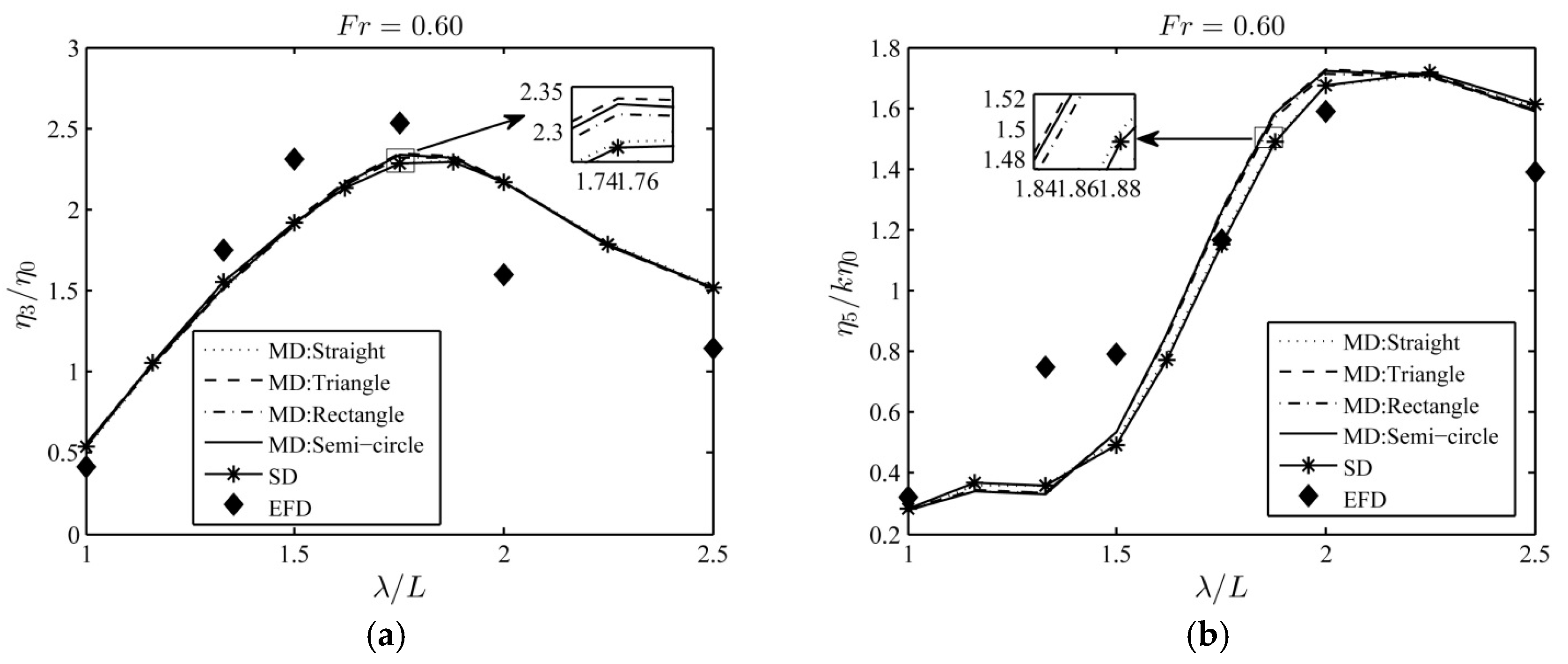
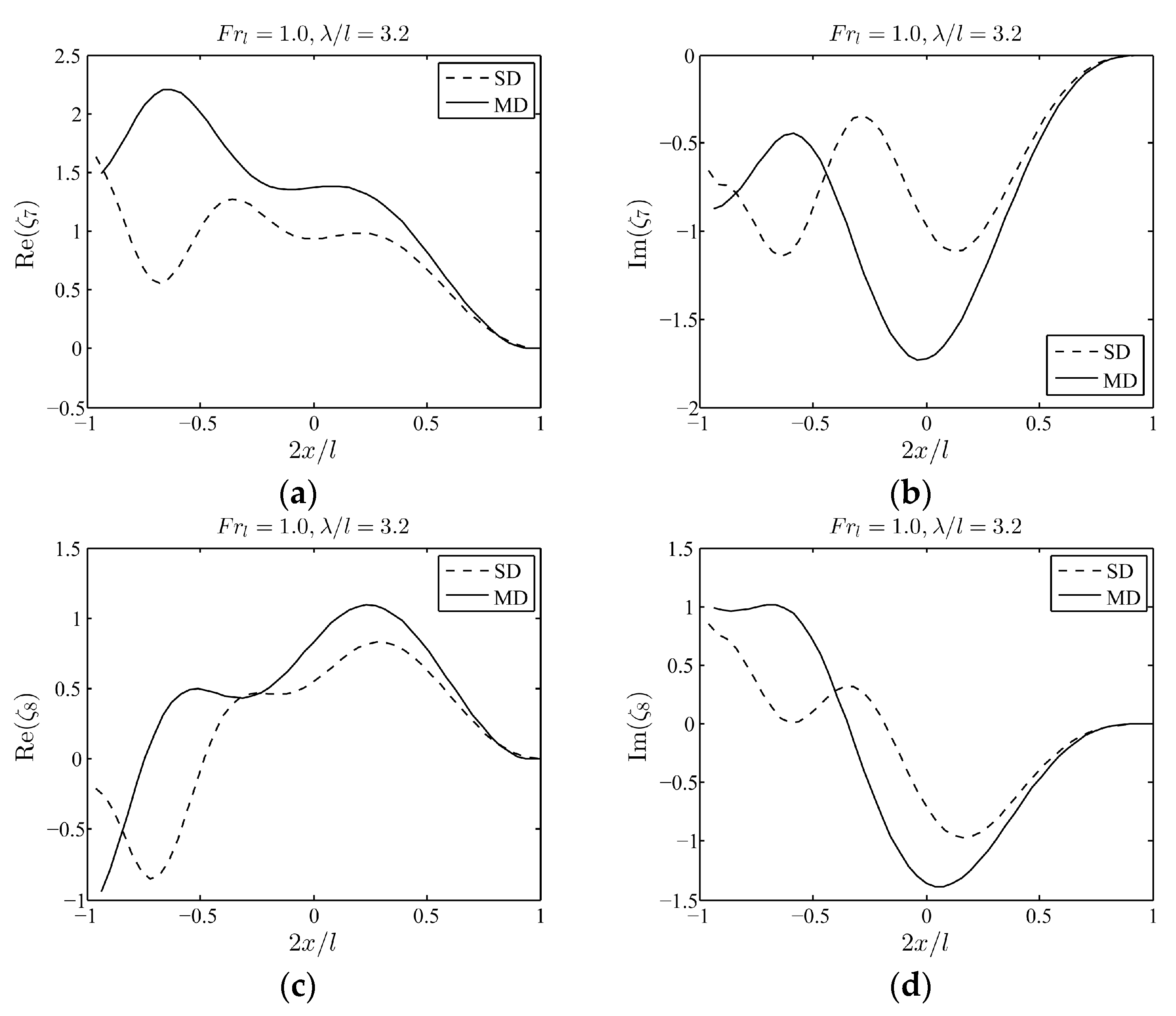
3.1. Validation of the Multi-Domain 2.5D Method

Before applying the multi-domain 2.5D method to an SES, the catamaran Delft 372 [16,17,18] is employed to validate this method. The Delft 372 [18] was firstly proposed by the Delft University of Technology as one of the “Standard Series” models for academic research. The principal parameters of the Delft 372 are listed in

Table 1. Main characteristics of the Delft 372 catamaran [16,17].

Parameters (symbol)	Value	Parameters (Symbol)	Value
Length between perpendiculars ($L$)	3.0 m	Longitudinal center of gravity ($x_{\mathrm{g}}$)	1.41 m
Beam overall ($B$)	0.94 m	Vertical center of gravity ($z_{\mathrm{g}}$)	0.34 m
Beam demihull ($b$)	0.24 m	Pitch radius of gyration ($k_{\mathrm{yy}}$)	0.782 m
Distance between center of demihulls ($d$)	0.70 m	Displacement ($∆$)	87.07 kg
Draft ($T$)	0.15 m	Moment of inertia for pitch ($I_{55}$)	53.245 kg·m2

.

As it is known, the level of the water surface between the demihulls of the Delft 372 catamaran is the same as that of the outside free surface. Thereby, the numerical results from the multi-domain 2.5D method with a splitter of an arbitrary shape should theoretically be the same as those obtained using the conventional single-domain 2.5D method, though numerical errors in calculations may occur.

As shown in Figure 3, four splitter shapes: (a) straight, (b) triangle, (c) rectangle, and (d) semicircle, are selected for the study. The splitters connect the lowest points of the demihulls. In Figure 3b, the vertical distance between the vertex of the triangle and the lowest point of the demihull is equal to $d$. In Figure 3c, the height of the rectangle is $d/2$.

The viscosity dissipation coefficient is set as $\nu =0$, since no viscous dissipation effects need to be considered in this case. Figure 4 depicts the heave and pitch RAO (response amplitude operator) of the Delft 372 advancing under Frouder number $Fr=0.60$ in regular head waves of wavelength $\lambda$. The lines labeled with “MD:Straight”, “MD:Triangle”, “MD:Rectangle”, and “MD:Semicircle” are numerical results from the multi-domain (MD) 2.5D method with straight, triangular, rectangular, an semicircular splitters, respectively. The lines labeled with “SD” and “EFD” are numerical results from the single-domain (SD) 2.5D method and results from experimental fluid dynamics (EFD) [16], respectively. Generally, it is desirable that all numerical results agree with the experimental ones. Nonetheless, one can observe that the numerical results from “MD:Straight” agree best with those from the single-domain 2.5D method. On the other hand, there exist notable discrepancies between the numerical results from “MD:Triangle”, “MD:Rectangle”, “MD:Semicircle” and the single-domain 2.5D method, which indicates that the multi-domain 2.5D method with triangular, rectangular, and semicircular splitters could induce slight numerical errors. It can be deduced that the numerical errors are positively associated with the length of the splitter.

The numerical results from this case suggest that the multi-domain 2.5D method developed in this paper is numerically stable, and that the straight design is the most suitable shape for the splitter.

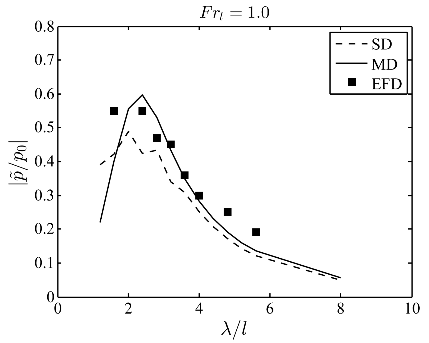
3.2. Multi-Domain 2.5D Method for the Hydrodynamics of an SES

The multi-domain 2.5D method with a straight splitter is employed to study an SES–partial air cushion supported catamaran (PACSCAT) [6]. The principal parameters of the PACSCAT are given in

Table 2. Main characteristics of the PACSCAT [6].

Parameters (symbol)	Value	Parameters (Symbol)	Value
Length overall ($L$)	3.0 m	Averaged trim $\left({\xi }_5\right)$	3.42°
Beam overall ($B$)	0.7 m	Moment of inertia for pitch ($M_{55}$)	77.4 kg·m2
Cushion length ($l$)	2.5 m	Static cushion overpressure $\left(p_0\right)$	760 Pa $\left(F_{rl}=0.73\right)$
Cushion breadth ($b$)	0.24 m	Air inflow rate $\left(Q_0\right)$	150 ${\mathrm{m}}^3/\mathrm{s}$
Displacement ($M$)	145 kg	Fan characteristic value $\left(\partial Q_{\mathrm{in}}/\partial p\right)$	−7.2 × 10−5 ${\mathrm{m}}^3/\left(\mathrm{s}·\mathrm{Pa}\right)$
Averaged sinkage $\left({\xi }_3\right)$	0.73 cm

. More details and the body plan for the PACSCAT can be found in Guo et al. [6]. Since the PACSCAT only runs in head waves, the variation of the fluctuating air pressure along the transverse direction can be ignored. Thereby, two orthogonal Fourier modes from Equation (2): $n_7\left(x,y\right)=1, n_8\left(x,y\right)=\sin \left(\mathsf{\pi }x/l\right)$ ($x_{\mathrm{m}}\cong 0$ for the PACSCAT) are sufficient for capturing the feature of the fluctuating air pressure. In addition, when the PACSCAT runs in waves, there exist averaged sinkage and trim for the hull, which are obtained from the experimental data [6] and given in Table 2. The plane of the interface in the multi-domain 2.5D method is approximately acquired by connecting the outer water surface at the bow and the averaged draft of air cushion at the center of gravity of the PACSCAT.

The strip panels of the PACSCAT for the single-domain and multi-domain 2.5D method are portrayed in Figure 5a,b, respectively. It can be observed that in Figure 5b the water level of the interface is lower than that of the outside free surface. One of most intuitive approaches to investigating the hydrodynamic effects of the water level difference is observing the radiation wave on the interface caused by fluctuating air pressure. If the water level difference has an impact on the hydrodynamics of the PACSCAT, the radiation wave obtained by the multi-domain 2.5D method should be different from that obtained by the single-domain 2.5D method. It is worth mentioning that the sidehulls of the PACSCAT have an “L” shape (see Figure 5), which could generate viscous effects when heaving or pitching in waves. Thereby, the viscosity dissipation coefficient is approximately set as $\nu =1\left(\mathrm{rad}/\mathrm{s}\right)$ for the single-domain and multi-domain 2.5D methods to compensate the viscous dissipation effects of the “L” shape sidehulls.

Figure 6 portrays the radiation wave profiles ${\zeta }_7,{\zeta }_8$ at the central longitudinal section $y=0$ of the interface due to the fluctuating air pressure of the PACSCAT advancing in waves of length $\lambda \left(\lambda /l=3.2\right)$ under Froude number $F_{rl}=1.0$. The waves ${\zeta }_7,{\zeta }_8$ can be calculated through Equation (15). The results “SD” and “MD” are obtained using the single-domain and multi-domain 2.5D methods, respectively.

From Figure 6, one can observe that the radiation wave obtained by the multi-domain 2.5D method is very different from that obtained using the single-domain 2.5D method, which suggests that the water level difference between the outside free surface and interface has a significant influence on the radiation wave on the interface, and the omission of the water level difference could bring inevitable errors to calculation of the the hydrodynamics of the PACSCAT. The numerical results also confirm the importance and necessity of applying the multi-domain 2.5D method to accurately predict the hydrodynamics of an SES.

In Figure 7, the numerical results on the fluctuating air pressure RAO of the PACSCAT are compared with the experimental ones “EFD” under $F_{rl}=1.0$. The results “SD” and “MD” are obtained using the single-domain and multi-domain 2.5D methods, respectively. From Figure 7, one can find that the fluctuating air pressure RAO from “MD” agrees better with “EFD” than “SD”. Moreover, “MD” varies more smoothly with wave length, while “SD” significantly oscillates in the vicinity of resonance waves.

The numerical results in this case suggest that the multi-domain 2.5D method can take water level difference into account and significantly improve the numerical results on the fluctuating air pressure.

4. Conclusions

This paper first presents a multi-domain 2.5D method for solving the hydrodynamics of an SES, whose water level of the interface is lower than that of the outside free surface. The novel multi-domain 2.5D method partitions the water domain into an outer domain and an inner domain, and keeps the potential and its derivative continuous on the adjacent boundaries of the two domains. The outer domain contains the outside free surface, while the inner domain includes the interface. The interface and the outside free surface are allowed to be at different water levels. Therefore, the multi-domain 2.5D method is able to precisely consider the water level difference in the SES.

The multi-domain 2.5D method is validated by predicting the motion response of a high-speed catamaran Delft 372 running in head waves, and the straight design is demonstrated to be an excellent splitter shape. Then, the multi-domain 2.5D method is employed to investigate the radiation wave on the interface of an SES (PACSCAT) caused by the fluctuating air pressure, and the numerical results suggest that the water level difference has a significant influence on the radiation wave. The multi-domain 2.5D method is also applied to solve the fluctuating air pressure RAO of the PACSCAT advancing in head waves, and the numerical results confirm that the multi-domain 2.5D method can improve the fluctuating air pressure of the PACSCAT.

The multi-domain concept proposed in this paper can be also applied to other free surface Green’s function methods to solve other hydrodynamic problems associated with multiple water levels.

References

1. Connell, S.B.; Milewski, M.W.; Goldman, B.; Kring, C.D. Single and multi-body surface effect ship simulation for T-Craft design evaluation. In Proceedings of the 11th International Conference on Fast Sea Transportation (FAST 2011), Honolulu, HI, USA, 26–29 September 2011; pp. 130–137. [Google Scholar]
2. García-Espinosa, J.; Capua, D.D.; Serván-Camas, B.; Ubach, P.A.; Oñate, E. A FEM fluid–structure interaction algorithm for analysis of the seal dynamics of a surface-effect ship. Comput. Methods Appl. Mech. Eng. 2015, 295, 290–304. [Google Scholar] [CrossRef] [Green Version]
3. Bhushan, S.; Mousaviraad, M.; Stern, F. Assessment of URANS surface effect ship models for calm water and head waves. Appl. Ocean Res. 2017, 67, 248–262. [Google Scholar] [CrossRef]
4. Sørensen, A.J.; Egeland, O. Design of ride control system for surface effect ships using dissipative control. Auromadca 1995, 31, 183–199. [Google Scholar] [CrossRef]
5. Bandas, J.C.; Falzarano, J.M. A numerical investigation into the linear seakeeping ability of the T-Craft. In Proceedings of the 11th International Conference on Fast Sea Transportation (FAST 2011), Honolulu, HI, USA, 26–29 September 2011; pp. 99–105. [Google Scholar]
6. Guo, Z.Q.; Ma, Q.W.; Yang, J.L. A seakeeping analysis method for a high-speed partial air cushion supported catamaran (PACSCAT). Ocean Eng. 2015, 110, 357–376. [Google Scholar] [CrossRef]
7. Xia, Z.; Shi, Y.; Cai, Q.; Wan, M.; Chen, S. Multiple states in turbulent plane Couette flow with spanwise rotation. J. Fluid Mech. 2018, 837, 477–490. [Google Scholar] [CrossRef]
8. Wang, J.; Ma, Q.W.; Yan, S.; Chabchoub, A. Breather rogue waves in random seas. Phys. Rev. Appl. 2018, 9. [Google Scholar] [CrossRef]
9. Guo, Z.Q.; Ma, Q.W.; Hu, X.F. Seakeeping analysis of a wave-piercing catamaran using URANS-based method. Int. J. Offshore Polar 2016, 26, 48–56. [Google Scholar] [CrossRef]
10. Shin, D.M.; Cho, Y. Diffraction of waves past two vertical thin plates on the free surface: A comparison of theory and experiment. Ocean Eng. 2016, 124, 274–286. [Google Scholar] [CrossRef]
11. Chen, X.B.; Duan, W.Y. Multi-domain boundary element method with dissipation. J. Mar. Sci. Appl. 2012, 11, 18–23. [Google Scholar] [CrossRef]
12. Faltinsen, O.; Zhao, R. Numerical predictions of ship motions at high forward speed. Philos. Trans. R. Soc. Lond. A 1991, 334, 241–252. [Google Scholar] [CrossRef]
13. Ma, S.; Duan, W.Y.; Song, J.Z. An efficient numerical method for solving “2.5D” ship seakeeping problem. Ocean Eng. 2005, 32, 937–960. [Google Scholar] [CrossRef]
14. Guo, Z.Q.; Ma, Q.W.; Qin, H.D. A time-domain Green’s function for interaction between water waves and floating bodies with viscous dissipation effects. Water 2018, 10, 72. [Google Scholar] [CrossRef]
15. Lee, C.H.; Newman, J.N. An extended boundary integral equation for structures with oscillatory free-surface pressure. Int. J. Offshore Polar 2015, 1, 347–353. [Google Scholar] [CrossRef]
16. Bouscasse, B.; Broglia, R.; Stern, F. Experimental investigation of a fast catamaran in head waves. Ocean Eng. 2013, 72, 318–330. [Google Scholar] [CrossRef]
17. Broglia, R.; Jacob, B.; Zaghi, S.; Stern, F.; Olivieri, A. Experimental investigation of interference effects for high-speed catamarans. Ocean Eng. 2014, 76, 75–85. [Google Scholar] [CrossRef]
18. Van’t Veer, R. Experimental Results of Motions and Structural Loads on the 372 Catamaran Model in Head and Oblique Waves; Technical Report, Report No. 1130; Delft University of Technology: Delft, The Netherlands, 1998. [Google Scholar]
Figure 1. Water flow domains Ω i , Ω e and their boundaries around the transverse section of an SES. The outer domain Ω e is surrounded by free surface S F , outer wetted surface S B e , splitter S C , and boundary at infinity S . The inner domain Ω i is enclosed by interface S P , inner wetted surface S B i , and splitter S C .
Water 10 00232 g001
Figure 2. Outer and inner domains and their extended domains. The coordinate system o e x e y e z e and o i x i y i z i are defined in the outer domain and inner domain, respectively. The origins o e and o i are located on the mean outside free surface S F and interface S P , respectively. (a) Outer domain Ω e and its extension Ω i e ; (b) Inner domain Ω i and its extension Ω e i .
Water 10 00232 g002
Figure 3. Various splitters for partitioning water domain around a transverse section of the Delft 372. (a) Straight splitter; (b) Triangular splitter; (c) Rectangular splitter; (d) Semicircular splitter.
Water 10 00232 g003
Figure 4. Comparison of motion response of the Delft 372 catamaran using the multi-domain 2.5D method with various splitters (straight, triangle, rectangle, semicircle) with results from single- domain 2.5D methods and experiments. λ is the wavelength. (a) Heave response amplitude operator (RAO); (b) Pitch RAO.
Water 10 00232 g004
Figure 5. Strip panels of the PACSCAT for the single-domain and multi-domain 2.5D method. (a) The strip panels for the single-domain 2.5D method, in which the interface and outside free surface are at the same water level; (b) The strip panels for the multi-domain 2.5D method, in which the interface is lower than the outside free surface.
Water 10 00232 g005
Figure 6. The comparison of profiles of radiation waves ζ 7 ,   ζ 8 on the interface due to fluctuating air pressure at y = 0 . The Froude number of the air cushion in the PACSCAT is F r l = 1.0 , and the wave length to air cushion length ratio is λ / l = 3.2 . (a) Real part of ζ 7 ; (b) Imaginary part of ζ 7 ; (c) Real part of ζ 8 ; (d) Imaginary part of ζ 8 .
Water 10 00232 g006
Figure 7. Comparison of fluctuating air pressure RAO of the PACSCAT using the multi-domain and single-domain 2.5D methods with experimental results.
Water 10 00232 g007