Article

Skin Effect of Fresh Water Measured Using Distributed Temperature Sensing

1
Department of Water Management, Water Resources Section, Delft University of Technology, Stevinweg 1, 2628CN, Delft, The Netherlands
2
Deltares, P.O. Box 177, 2600 MH Delft, The Netherlands
3
Department of Biological and Ecological Engineering, Oregon State University, 116 Gilmore Hall, Corvallis, OR 97331, USA
*
Author to whom correspondence should be addressed.
Water 2018, 10(2), 214; https://doi.org/10.3390/w10020214
Submission received: 5 December 2017 / Revised: 5 February 2018 / Accepted: 11 February 2018 / Published: 16 February 2018

Abstract

:
A phenomenon known as the skin effect—a layer of surface water that is colder than the water beneath it—was previously described in oceanography and verified in lab measurements. Only a few measurements have been done on the skin effect in field conditions, and therefore this phenomenon is relatively unknown. This paper presents measurements of the skin effect for three fresh water bodies in the Netherlands, Israel and Ghana. Using Distributed Temperature Sensing, high temporal and spatial resolution measurements were made below, at and above the air–water surface. Measurements presented in this study suggest that the skin effect of fresh water bodies is predominantly a daytime phenomenon and only occurs during low to zero wind speeds. The thickness of the skin effect was measured to be an order of magnitude larger than the previously assumed less than 1 mm.

1. Introduction

Estimations of the energy balance of lakes and reservoirs are important to determine their heating and cooling processes, as the (thermo)dynamics of lakes and reservoirs and their water balance are significantly influenced by the surface energy fluxes [1,2,3,4]. Previous studies showed a clear temperature drop at the air–water interface [3,5,6,7]. At first, we assumed that this was in fact the wet bulb temperature due to splashing of water on the measurement setup. However, the lower temperatures are below the water surface, which suggests the occurrence of an infrared and evaporation driven skin effect.
The skin effect refers to a thin, more or less stable layer of surface water that is colder than the water beneath it due to radiative energy loss that exceeds the replenishment of energy via shortwave absorption or thermal diffusion from the lower water. As the energy transfer from water to atmosphere (evaporation, long-wave radiation, or sensible heat) happens at the surface, a thin cold layer is created (the skin effect) [8,9]. In natural lakes, the upwelling long-wave radiation dominates long-wave energy transfer. This is due to the surface supplying all outgoing long-wave energy, while incoming shortwave energy is absorbed through the first meters of the water column. The thickness of the skin layer is hypothesised to be regulated by conductive and diffusive heat processes [10]. Detailed analysis about the heat exchange and energy transfer over the water surface can be found in [11].
Existence of a skin effect results from low turbulence close to the water surface compared to the layers below. In cases where density is inverted and far from interfaces in water, heat is most rapidly transferred by turbulent mixing. Close to the surface, however, low Reynolds numbers suppress turbulence, and thus viscous forces and molecular processes prevail. Thus, the heat from lower water layers is only transferred to the laminar top layer by molecular conduction, which is an order of magnitude less efficient than turbulent mixing [12].
A colder layer of water on the surface is a documented phenomenon in oceanography and most research about the skin effect of water bodies has been focused on oceans [8,13,14]. The greater of research focussed on skin effect in oceanography as compared to fresh water reservoirs is related to the fact that the surface of oceans is particularly interesting from biological and chemical perspective. The top 0–1 mm of ocean surfaces contains a higher concentration of bacteria and larvae, as well as having elevated concentrations of non-polar molecules attracted to the air–water interface [15,16].
A few studies measured the skin effect in lakes as well [17,18]. Available studies on the skin effect agree that the colder layer can be present during both day and night, and that the temperature difference between the skin and the temperature of underlying water ( Δ T w a t e r ) is highest during the daytime [18,19]. However, to date, there have been few analyses that have investigated under which conditions it occurs, and what affects the skin effect magnitude. In this paper, we use novel measurements to also analyze and discuss the timing of occurrence of the skin effect.
Although the skin effect has been previously measured (e.g., [13,14,19,20]), the measurements of the skin effect thickness remain scarce. Previous work on the skin effect thickness suggested that the effect is limited to about one millimeter. However, until now, no measurements of skin effect of fresh water were done under field conditions. For example, Grassl [21] derived the thickness of the skin effect mathematically, Duan et al. [22] used saturation vapour pressure measurements from funnel measurements, and Hisatake et al. [23] performed measurements under laboratory conditions by lowering a thermocouple into water and then retrieving it again. In laboratory conditions, one could never reach the prevailing outgoing longwave radiation, as is typical for open sky. Our paper presents a first analysis based on high-resolution field measurements obtained from three different measurement campaigns.
This paper aims to quantify the skin effect of natural water bodies. We present high-resolution temperature measurements of air–water interface from three different locations using Distributed Temperature Sensing (DTS), and discuss potential explanations for the observed phenomena.

2. Materials and Methods

Goals of the methodology are to obtain high-resolution measurements of the skin effect and link them to the development of the skin temperature. In this section, we first introduce the measurement technique and the way we defined the variables such as the skin temperature and thickness; later, we describe the specifics of each measurement site.

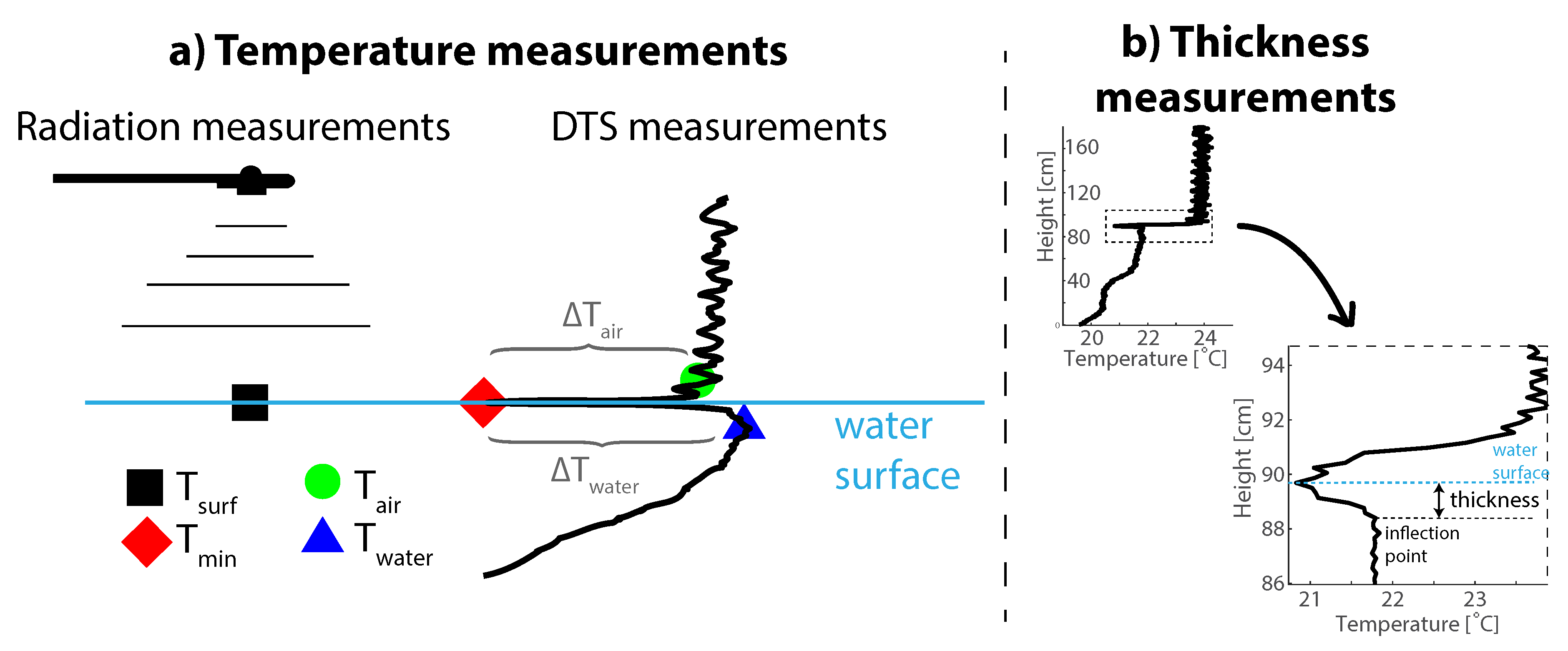
2.1. High-Resolution Measurements

DTS was used to measure vertical temperature profiles at very high-resolution in three different locations. DTS is a method that allows for high-resolution temperature measurements in air [24,25], water [3,26,27], and soil [28,29]. The method is based on backscatter of light traveling through a fiber optic cable. The ratio between backscatter of various wavelengths is indicative of the temperature along the cable. More details about the DTS method can be found in [7,30].
The resolution of DTS can be increased by wrapping the fibre optic cable around an auxiliary construction [7,31]. In this research, we are using two types of auxiliary constructions, both allowing for measuring the vertical temperature with sub-centimeter resolution. However, attaching cables to a construction can introduce an error in observed air temperature values. The effect of the construction on the measurements can be found in [32].

2.2. Measured and Calculated Variables

Continuous measurements of air–water interface resulted in temperature profiles similar to the one seen in Figure 1a. We define the bulk water temperature (T w a t e r [°C]) as the average temperature over ∼0.10 m below the water surface, air temperature (T a i r [°C]) as the average temperature over ∼0.10 m above the water surface, and the skin temperature as the measured minimum temperature (T m i n [°C]).
Δ T w a t e r represents the difference between the bulk temperature of water (T w a t e r ) and the measured minimum temperature (T m i n ). Δ T a i r represent the difference between the bulk temperature of air (T a i r ) and the measured minimum temperature (T m i n ):
Δ T a i r = T a i r T m i n ,
Δ T w a t e r = T w a t e r T m i n .
We define the temperature drop as the smaller of the two thermal gradients found in the water Δ T w a t e r and air Δ T a i r immediately above and below the air–water interface:
Δ T d r o p = m i n ( Δ T w a t e r , Δ T a i r ) .
When there is no thermal skin layer ( Δ T d r o p = 0), T m i n is defined as equal to the surface temperature.
A second important parameter measured at the water surface was the thickness of the skin layer. The thickness was defined as the distance between the minimum measured temperature (T m i n ) and the point where the local numerical derivative of the water temperature changed from negative to positive values (Figure 1b); in other words, the place where the water temperature does not increase any more compared to the above laying measurement.

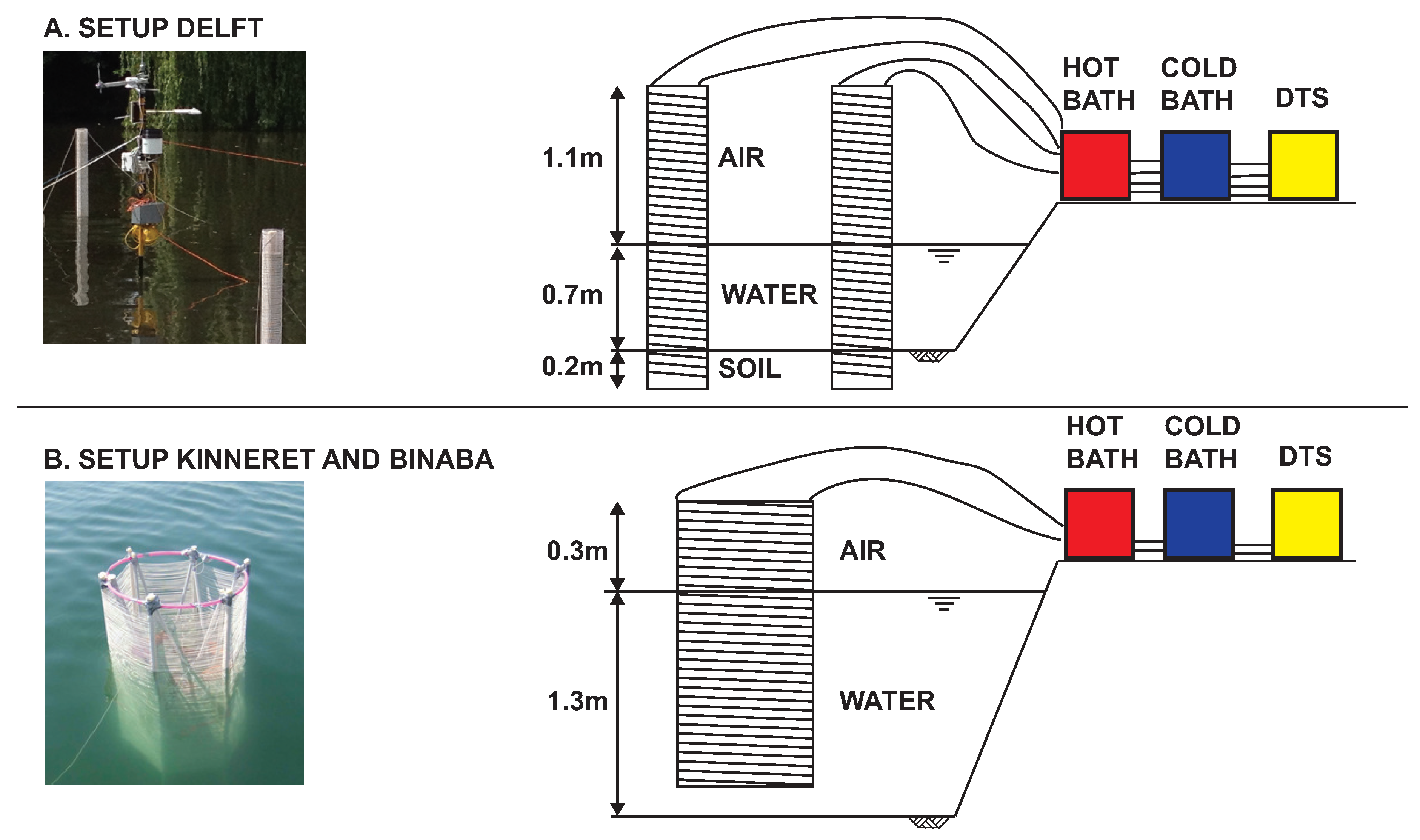
2.3. Measurement Locations and Monitoring Equipment

Three datasets were used in this research, one from an urban pond in Delft (The Netherlands), one from Lake Binaba in Ghana, and one from Lake Kinneret in Israel. All three datasets included a high-resolution temperature profile of water–air interface. Data from Delft and Israel also included meteorological observations. In the following, the measurements setups will be discussed briefly. More detailed descriptions can be found in [3,32].

2.3.1. Delft Pond

Measurements took place from 12 July through 7 August 2014 in a shallow urban pond at the Amalia van Solmslaan in Delft, the Netherlands (52.007° N, 4.375° E). The climate of Netherlands is moderate oceanic with summer starting in June and ending mid-September. Average water depth in the pond is 0.7 m and the average area of water surface is 3627 m 2 . The pond is located between a 3-story office building to the north and a residential building to the south, while the street, trees, and the largest part of the pond are located on the west side.
For DTS, a Silixa Ultima (Silixa Ltd., Hertfordshire, UK) with spatial resolution of 0.3 m was used. The sampling resolution in the glass fibre cable was set to 0.126 m (to satisfy the Nyquist criteria for spatial resolution) and the temporal resolution 5 min. Double ended calibration [33] was used including two calibration baths, one with unheated water and one with water heated to ∼35 °C. The temperatures in the calibration baths were measured with two Pt100 temperature probes built into the DTS.
A vertical temperature profile was measured at two locations in the northeast corner of the pond. An optical cable (AFL 1.6 mm simplex 50/125, white) was wrapped around a 200 cm long transparent PVC tube with 11 cm diameter resulting in ∼2 mm vertical resolution of the temperature measurements (Figure 2a). To ensure ventilation, four 2 cm diameter holes were drilled into the tube every 6–8 cm. Each temperature profile covered ∼20 cm of the mud on the bottom of the pond, 70 cm of water, and 110 cm of air. The same type of optical cable was used for all three measurement locations.
Air temperature, relative humidity, wind speed, wind direction, and precipitation were measured using a standard HOBO weather station (Onset Computer CO., Bourne, MA, USA) in the middle of the pond. Additionally, incoming and outgoing short- and long-wave radiation were measured using a CNR4 net radiometer (Kipp & Zonen, Delft, The Netherlands).
The measurements in Delft also included longwave outgoing radiation, which allowed for calculation of the surface temperature (T s u r f ) using the Stefan–Boltzmann law:
R l o u t = σ ϵ T s u r f 4 ,
where Rl o u t is the measured outgoing longwave radiation [Wm 2 ], T is the surface temperature [K], ϵ = 0.98 [-] is the emissivity of water [34] and σ = 5.67 × 10 8 Wm 2 K 4 is the Stefan–Boltzmann constant.
A parameter influencing the calculated surface temperature is the emissivity of the water. Emissivity decreases with higher sediment concentration in water; for highly turbid salty water, it can drop down to 0.95 [34]. The turbidity of the urban pond in Delft was not measured. Therefore, we performed a sensitivity analysis of the surface temperature to emissivity. With decreasing emissivity values, the calculated surface temperatures increased. As a consequence, the T s u r f could change by up to 2.8 K depending on the chosen emissivity value. For this analysis, the value 0.98 was chosen based on the fact that the measurements were taken in and above highly turbid fresh water body, as suggested in the literature [34].

2.3.2. Lake Binaba

Measurements in Lake Binaba were taken between 24 and 28 October 2011. The climate of northern Ghana (10.78° N, 0.48° W), where the lake is located, is tropical with a dry and wet season. During the rainy season, April to September, the lake is fed by runoff via natural streams. Lake Binaba is a small artificial lake with average depth 3 m and lake surface 4.5 km 2 . Water from the lake is used for small-scale irrigation and domestic water use.
A four-meter resolution Halo DTS Sensor (Sensornet, Hertfordshire, UK) was used at this site. The sampling resolution was 2.03 m and temporal averaging 2 min. Double-ended calibration was used including two calibration baths, one with unheated water and one with water heated to ∼35 °C. Two HOBO Tidbit Mini Underwater Temperature Data loggers (Onset Computer CO.) with a logging interval of 1 min were used to measure the temperature in the calibration baths.
Vertical temperature profiles were measured in the pond using an open construction. A fiber-optic cable was wrapped around a PVC hyperboloid frame (Figure 2b) constructed from PVC pipes. Extra weight was added to the bottom of the frame to counteract the buoyancy caused by air trapped in the PVC pipes. The open construction of the setup ensured low influence of direct solar radiation, and free flow of water and air through the construction. The vertical resolution created by wrapping the wire around the construction was ∼4 mm.

2.3.3. Lake Kinneret
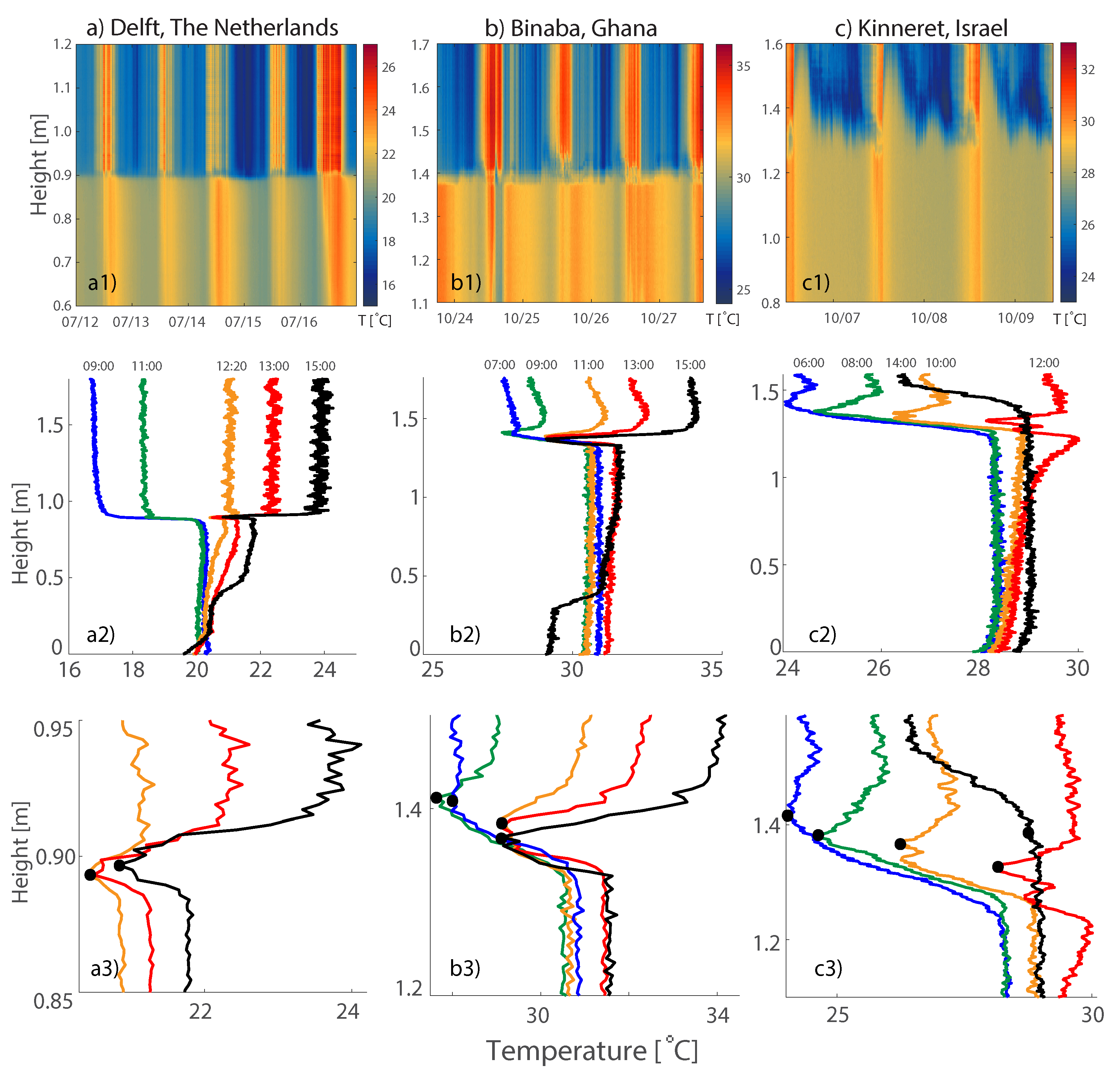
Measurements in Lake Kinneret (32.78° N, 35.59° E) took place between 6 and 9 October 2011. Climate of northern Israel is warm Mediterranean with a colder rainy season between October and April. Lake Kinneret has an average lake surface of 166 km 2 . During the experiment, a northwesterly sea breeze formed each afternoon and usually peaked at 3:00 p.m. local time with wind speed of ∼5–10 m/s. The wind was significantly lower for the rest of the day: <2 m/s from 8:00 p.m. until 12:00 p.m. the following day.
An Oryx (Sensornet) with two-meter resolution was used to record the temperature with spatial samples averaging 1.03 m and temporal averaging 1 min. Single ended calibration [35] was used including two calibration baths. Temperature in the calibration baths, as well as the temperature measurement method, was the same as for the measurements taken in Lake Binaba. Additionally, the setup used was the same for both Binaba and Kinneret. However, a higher sampling resolution of the Oryx DTS machine resulted in vertical resolution of ∼2 mm.
A meteorological station was placed in the middle of Lake Kinneret. Air temperature, relative humidity (both probe model 43372C, R.M. Young), wind speed and wind direction (MA-05106 wind monitor, R.M. Young) were measured in 10 min intervals.

3. Results

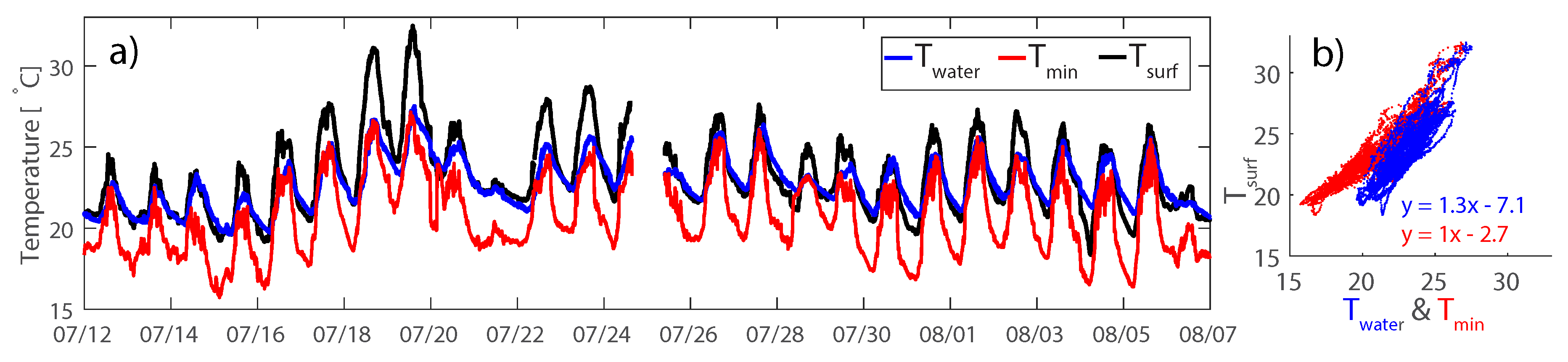
3.1. Surface Temperature

Comparison of the calculated surface temperature (T s u r f ) and two temperatures measured using DTS (T w a t e r and T m i n ) can be seen in Figure 3a. At night, T s u r f followed the measured water temperature (T w a t e r ); however, during the day, T s u r f reached on average 0.6 K higher values than T w a t e r . Average temperature of T s u r f and T w a t e r over the whole measurement period was 23.3 °C and 23.0 °C, respectively. Average measured T m i n reached only 20.6 °C. This might suggest that T w a t e r is a better approximation of the surface temperature than T m i n . However, T m i n followed the variation of T s u r f and the amplitude of its diurnal change almost exactly, with an offset of 2.7 K. The minimum temperature (T m i n ) measured proved to be well correlated with the surface temperature (T s u r f ) calculated from outgoing longwave radiation measurements for the Delft location using Equation (4). The offset of 2.7 K is well in the accuracy range of the pyrgometer that recorded the outgoing longwave radiation used for the calculation of the surface temperature. Figure 3b shows a scatter plot of the calculated surface temperature (y-axis) and T m i n and T w a t e r . Correlation coefficients of T s u r f and the two temperatures measured using DTS were 0.86 for T m i n and 0.68 for T w a t e r .
All measurements showed a temperature decrease close to the water surface during the day (Figure 4). In general, the temperature drop followed a diurnal pattern at all three locations. Maximum values were reached between 12:00 p.m. and 4:00 p.m. in Delft and between 11:00 a.m. and 2:00 p.m. in Kinneret. At the Binnaba location, the maximum temperature differences occurred at a different time on each of the four measurement days. At night, the anomaly disappeared.

3.2. Energy Balance of Water Surface

The observed total thickness of the colder layer of water was measured to be up to 3 cm (Figure 5). Existence of a colder layer of water on top of warm water creates instability. The cold layer will periodically mix with the warmer water below through finger-like structures [36].
The creation of a colder layer of water near the water surface can be approached from the energy-balance point of view. If the average temperature drop ( Δ T d r o p ) of the top 3 cm is ∼1 K, and the heat capacity of water equals 4.2 kJ kg 1 K 1 , the energy deficit compared to the water below is about 126 kJm 2 . The heat flux Q [Wm 2 ] between the warm and cold water layer can be calculated using:
Q = K w a t e r A d T d z ,
where K w a t e r = 0.58 Wm 1 K 1 is the thermal conductivity of water, A = 1 m 2 is the unit area, and d T d z [Km 1 ] is temperature gradient over depth. With a temperature gradient of ∼1 K over 3 cm, the flux is ∼20 Wm 2 .
The average net longwave radiation measured at the location in Delft during a day was –50 Wm 2 , meaning there was a radiative flux from water to the air. If we assume the water was cooled by the radiative flux only and the flux from water to the top layer is 20 Wm 2 , the time to extract 126 kJ by a 30 Wm 2 flux is computed to be 70 min. Indeed, the temperature difference of the top layer shows fluctuations in time. Local minima in the temperature difference ( Δ T d r o p ) occurred on average once every 25 to 95 min (Figure 6). The instantaneous differences in time periods are caused by turbulent fluxes: evaporation and sensible heat, which were not investigated in this research.

4. Discussion

We have presented measurements of a localized, transient surface temperature drop found at the air–water interface at different locations with three different climates. For the Delft case, we have compared it to the surface temperature calculated from long wave radiation observations. Our measurements suggest that this temperature anomaly is the skin effect, as the minimum temperature occurs at the water–air interface.
A skin effect is not the only possible explanation for occurrence of a temperature drop close to the water surface. Another possible explanation is a measurement artifact caused by the splashing of water on our sensor systems. Small waves could continuously wet the optical fiber of the measurement setup, which would consequently record temperature similar to wet bulb temperature. Waves on the water surface of lakes and ponds are generally created by wind. Figure 7 shows a daily occurrence of the temperature drop, and its size ( Δ T d r o p ), and the wind speed. Both data sets show that, with higher wind speeds, the temperature difference decreased, or even disappeared totally.
Figure 7 convincingly illustrates that the recorded minimum is not related to splashing water or wet bulb temperature. It is possible that, at some occasions, especially during moments with wind speeds above zero (e.g., Figure 7a in the evening of 14 July), splashing of water is what is causing the temperature to appear colder close to water surface. This also corresponds with the fact that the correlation of the minimum temperature measured by DTS in Delft (T m i n ) with calculated water surface temperature (T m i n ) was weaker at times with higher wind speeds.
Interestingly though, the calculated water surface temperature had an offset of 2.7 K compared to the measured skin temperature. As mentioned before, this offset is within the range of precision of the pyrgeometer used. Nonetheless, the proximity of the buildings surrounding the pond might have had an additional effect on the radiation measurements as well. During the daytime and especially early evening hours, the surface temperature of the buildings was higher than the temperature of the pond. The additional longwave radiation from the walls of the buildings could have contributed to the recorded longwave radiation of the pond.
However, it remains to be investigated how weather conditions and the physical properties of the water body influence the occurrence, size, and disappearance of the temperature drop. For example, although the temperature drop was predominantly measured during daytime, occasionally it persisted over night. This situation was mostly visible during very warm nights, when the air temperature stayed higher than the water temperature. This suggests that creation and existence of this temperature drop is dependent on the differences between the water and air temperature. A similar conclusion can be drawn by observing the temperature profile in Figure 4. The decrease in temperature ( Δ T d r o p ) appeared when the air temperature reduced the water temperature.
Another aspect that seems to play an important role is the wind. Our measurements show that during periods with high wind speed, the skin effect disappeared. This might seem contradictory to the assumption that evaporative cooling contributes to creation of the skin effect, as wind would enhance evaporation. On the other hand, high wind speed can disturb the surface layer and promote better mixing throughout the top few centimeters of water.
There seem to be a difference in the thickness of the skin effect between the urban pond in Delft (ca 1.5 cm) and the two bigger lakes. This could be caused by several factors, such as transparency of the water, depth, or possible wave formation on the bigger lakes. These variables were not measured at either location. More research is needed to investigate what drives the thickness of the skin effect.
DTS proved to be a suitable method for measuring the skin effect. Wrapping the optical fiber in a more compact method and by increasing the diameter of the auxiliary construction allowed for higher resolution. Another advantage of this method is the continuity of the measurements allowing for a fuller observation of temporal changes in the skin effect and temperature gradient over the top layer of water. A simple energy balance calculation showed that the measured timescale and magnitude of the energy exchange is indeed comparable to the calculated values for the temperature gradient measured in Delft.
When using fiber optic cable for near water surface measurements, one needs to be aware of its tendency to absorb solar radiation, despite its white colour. This effect can be partly visible in Figure 1a and Figure 4c3, where the DTS is measuring higher temperature just below the surface compared to the air temperature. The effect of radiation on DTS measurements in air and water close to the water surface was described in [32] and [6], respectively. Nonetheless, even with this effect, skin is still detected, but it may, on some occasions, appear thicker due to the way the thickness is defined.
Further research of the skin effect in fresh water is necessary in order to understand how, and under what conditions, is the cold layer created, and when it mixes with the underlying warmer water. It is possible that the auxiliary construction of the DTS setup created a preferential flow during the moments when the cold layer mixed. This would cause the measured cold layer to appear thicker than the actual skin layer. Nonetheless, the thickness of the skin layer still needs to be investigated in more detail, as there are only few references available [22,23]. Additionally, higher vertical resolution of the temperature measurements should be employed in future investigations. The 2 mm resolution, as used in this study, could not detect features at the sub-millimeter scale, so we cannot directly relate our measurements to features in the skin layer of less than 1 mm, as mentioned in [8,9,18,19].

5. Conclusions

Analysis of data collected from three different measurement locations confirmed that the measured temperature drop could be attributed to the skin effect, rather than wet bulb temperature due to splashing of water. For the first time, the skin effect was measured consistently under field conditions in fresh water bodies. Our data suggest that the skin effect of fresh water bodies is predominantly a daytime phenomenon and only occurs during low to zero wind speeds.
The high-resolution DTS measurements provided an important insight into the surface energy balance dynamics of water bodies by allowing observation of the temperature drop below the air–water interface during the three field studies.
Measurements presented in this study suggest that the thickness of the skin effect is larger than the previously assumed 1 mm or less [8,18,23]. It was observed to be on the order of 3 cm in thickness. This sheds a new light on the energy balance dynamics around the air–water interface of water bodies. Specifically, our measurements suggest that inaccurate description of the skin effect layer might result in errors in modelling water body energy and heat fluxes, as they differ for the water body itself and for the skin layer.

Acknowledgments

This research is part of a Climate KIC research project Blue-Green Dream, investigating the cooling effects of blue-green climate adaptation measures in urban areas. We would like to thank Gordon L. Godshalk and Catherine van der Lely for language editing.

Author Contributions

A.S. and T.v.E. designed measurement setup and experiments; A.S. and T.v.E. performed experiments; A.S., J.S., F.v.d.V. and N.v.d.G. analyzed data; A.S. wrote the intial paper; and all contributed to writing the paper.

Conflicts of Interest

The authors declare no conflict of interest.

References

  1. Henderson-Sellers, B. Calculating the surface energy balance for lake and reservoir modeling: A review. Rev. Geophys. 1986, 24, 625–649. [Google Scholar] [CrossRef]
  2. Tanny, J.; Cohen, S.; Assouline, S.; Lange, F.; Grava, A.; Berger, D.; Teltch, B.; Parlange, M. Evaporation from a small water reservoir: Direct measurements and estimates. J. Hydrol. 2008, 351, 218–229. [Google Scholar] [CrossRef]
  3. Van Emmerik, T.; Rimmer, A.; Lechinsky, Y.; Wenker, K.; Nussboim, S.; Van de Giesen, N. Measuring heat balance residual at lake surface using Distributed Temperature Sensing. Limnol. Oceanogr. Methods 2013, 11, 79–90. [Google Scholar] [CrossRef]
  4. Nordbo, A.; Launiainen, S.; Mammarella, I.; Leppäranta, M.; Huotari, J.; Ojala, A.; Vesala, T. Long-term energy flux measurements and energy balance over a small boreal lake using eddy covariance technique. J. Geophys. Res. Atmos. 2011, 116. [Google Scholar] [CrossRef]
  5. Solcerova, A.; van de Ven, F.; van de Giesen, N. Nighttime cooling of an urban pond. submitted.
  6. Vercauteren, N.; Huwald, H.; Bou-Zeid, E.; Selker, J.S.; Lemmin, U.; Parlange, M.B.; Lunati, I. Evolution of superficial lake water temperature profile under diurnal radiative forcing. Water Resour. Res. 2011, 47. [Google Scholar] [CrossRef] [Green Version]
  7. Selker, J.S.; Thevenaz, L.; Huwald, H.; Mallet, A.; Luxemburg, W.; Van De Giesen, N.; Stejskal, M.; Zeman, J.; Westhoff, M.; Parlange, M.B. Distributed fiber-optic temperature sensing for hydrologic systems. Water Resour. Res. 2006, 42. [Google Scholar] [CrossRef] [Green Version]
  8. Minnett, P.J.; Smith, M.; Ward, B. Measurements of the oceanic thermal skin effect. Deep Sea Res. Part II Top. Stud. Oceanogr. 2011, 58, 861–868. [Google Scholar] [CrossRef]
  9. Fairall, C.; Bradley, E.F.; Godfrey, J.; Wick, G.; Edson, J.B.; Young, G. Cool-skin and warm-layer effects on sea surface temperature. J. Geophys. Res. 1996, 101, 1295–1308. [Google Scholar] [CrossRef]
  10. Saunders, P.M. The temperature at the ocean-air interface. J. Atmos. Sci. 1967, 24, 269–273. [Google Scholar] [CrossRef]
  11. Edinger, J.E.; Brady, D.K.; Geyer, J.C. Heat Exchange and Transport in the Environment; Report No. 14; Technical Report; Department of Geography and Environmental Engineering, Johns Hopkins University: Baltimore, MD, USA, 1974. [Google Scholar]
  12. Ward, B.; Minnett, P.J. An autonomous profiler for near surface temperature measurements. In Gas Transfer at Water Surfaces; Springer Science & Business Media: Berlin, Germany, 2002; pp. 167–172. [Google Scholar]
  13. Ridley, I.K.; Lawrence, S.P.; Llewellyn-Jones, D.T.; Parkes, I.M.; Yokoyama, R.; Tanba, S.; Oikawa, S. Use of ATSR-measured ocean skin temperatures in ocean and atmosphere models. In Proceedings of the Third ERS Symposium on Space at the Service of Our Environment, Florence, Italy, 14–21 March 1997; pp. 1317–1321. [Google Scholar]
  14. Kang, H.J.; Yoo, J.M.; Jeong, M.J.; Won, Y.I. Uncertainties of satellite-derived surface skin temperatures in the polar oceans: MODIS, AIRS/AMSU, and AIRS only. Atmos. Meas. Tech. 2015, 8, 4025–4041. [Google Scholar] [CrossRef]
  15. Hardy, J. The sea surface microlayer: Biology, chemistry and anthropogenic enrichment. Prog. Oceanogr. 1982, 11, 307–328. [Google Scholar] [CrossRef]
  16. Bidleman, T.; Olney, C. Chlorinated hydrocarbons in the Sargasso Sea atmosphere and surface water. Science 1974, 183, 516–518. [Google Scholar] [CrossRef] [PubMed]
  17. Woodcock, A.H.; Stommel, H. Temperatures Observed Near the Surface of a Fresh-Water Pond at Night. J. Atmos. Sci. 1947, 4, 102–103. [Google Scholar] [CrossRef]
  18. Wilson, R.C.; Hook, S.J.; Schneider, P.; Schladow, S.G. Skin and bulk temperature difference at Lake Tahoe: A case study on lake skin effect. J. Geophys. Res. Atmos. 2013, 118. [Google Scholar] [CrossRef]
  19. Schluessel, P.; Emery, W.J.; Grassl, H.; Mammen, T. On the bulk-skin temperature difference and its impact on satellite remote sensing of sea surface temperature. J. Geophys. Res. Oceans 1990, 95, 13341–13356. [Google Scholar] [CrossRef]
  20. Jessup, A.; Branch, R. Integrated ocean skin and bulk temperature measurements using the calibrated infrared in situ measurement system (CIRIMS) and through-hull ports. J. Atmos. Ocean. Technol. 2008, 25, 579–597. [Google Scholar] [CrossRef]
  21. Grassl, H. The dependence of the measured cool skin of the ocean on wind stress and total heat flux. Bound. Layer Meteorol. 1976, 10, 465–474. [Google Scholar] [CrossRef]
  22. Duan, F.; Thompson, I.; Ward, C. Statistical rate theory determination of water properties below the triple point. J. Phys. Chem. B 2008, 112, 8605–8613. [Google Scholar] [CrossRef] [PubMed]
  23. Hisatake, K.; Tanaka, S.; Aizawa, Y. Evaporation rate of water in a vessel. J. Appl. Phys. 1993, 73, 7395–7401. [Google Scholar] [CrossRef]
  24. Euser, T.; Luxemburg, W.; Everson, C.; Mengistu, M.; Clulow, A.; Bastiaanssen, W. A new method to measure Bowen ratios using high-resolution vertical dry and wet bulb temperature profiles. Hydrol. Earth Syst. Sci. 2014, 18, 2021–2032. [Google Scholar] [CrossRef] [Green Version]
  25. De Jong, S.; Slingerland, J.; Van de Giesen, N. Fiber optic distributed temperature sensing for the determination of air temperature. Atmos. Meas. Tech. 2015, 8, 335–339. [Google Scholar] [CrossRef]
  26. Westhoff, M.; Savenije, H.; Luxemburg, W.; Stelling, G.; Van de Giesen, N.; Selker, J.; Pfister, L.; Uhlenbrook, S. A distributed stream temperature model using high-resolution temperature observations. Hydrol. Earth Syst. Sci. 2007, 11, 1469–1480. [Google Scholar] [CrossRef] [Green Version]
  27. Sebok, E.; Duque, C.; Kazmierczak, J.; Engesgaard, P.; Nilsson, B.; Karan, S.; Frandsen, M. High-resolution distributed temperature sensing to detect seasonal groundwater discharge into Lake Væng, Denmark. Water Resour. Res. 2013, 49, 5355–5368. [Google Scholar] [CrossRef]
  28. Steele-Dunne, S.; Rutten, M.; Krzeminska, D.; Hausner, M.; Tyler, S.; Selker, J.; Bogaard, T.; Van de Giesen, N. Feasibility of soil moisture estimation using passive distributed temperature sensing. Water Resour. Res. 2010, 46. [Google Scholar] [CrossRef] [Green Version]
  29. Bense, V.; Read, T.; Verhoef, A. Using distributed temperature sensing to monitor field scale dynamics of ground surface temperature and related substrate heat flux. Agric. For. Meteorol. 2016, 220, 207–215. [Google Scholar] [CrossRef]
  30. Tyler, S.W.; Selker, J.S.; Hausner, M.B.; Hatch, C.E.; Torgersen, T.; Thodal, C.E.; Schladow, S.G. Environmental temperature sensing using Raman spectra DTS fiber-optic methods. Water Resour. Res. 2009, 45. [Google Scholar] [CrossRef] [Green Version]
  31. Hilgersom, K.; van de Giesen, N.; de Louw, P.; Zijlema, M. Three-dimensional dense distributed temperature sensing for measuring layered thermohaline systems. Water Resour. Res. 2016, 52, 6656–6670. [Google Scholar] [CrossRef]
  32. Hilgersom, K.; Van Emmerik, T.; Solcerova, A.; Berghuijs, W.; Selker, J.; Van de Giesen, N. Practical considerations for enhanced-resolution coil-wrapped Distributed Temperature Sensing. Geosci. Instrum. Method. Data Syst. 2016, 5, 151–162. [Google Scholar] [CrossRef]
  33. Van De Giesen, N.; Steele-Dunne, S.C.; Jansen, J.; Hoes, O.; Hausner, M.B.; Tyler, S.; Selker, J. Double-ended calibration of fiber-optic Raman spectra distributed temperature sensing data. Sensors 2012, 12, 5471–5485. [Google Scholar] [CrossRef] [PubMed]
  34. Wen-Yao, L.; Field, R.; Gantt, R.; Klemas, V. Measurement of the surface emissivity of turbid waters. Remote Sens. Environ. 1987, 21, 97–109. [Google Scholar] [CrossRef]
  35. Hausner, M.B.; Suárez, F.; Glander, K.E.; Giesen, N.v.d.; Selker, J.S.; Tyler, S.W. Calibrating single-ended fiber-optic Raman spectra distributed temperature sensing data. Sensors 2011, 11, 10859–10879. [Google Scholar] [CrossRef] [PubMed]
  36. Hilgersom, K.; Zijlema, M.; van de Giesen, N. An axisymmetric non-hydrostatic model for double-diffusive water systems. Geosci. Model Dev. 2018, 11, 521–540. [Google Scholar] [CrossRef]
Figure 1. (a) schematization of temperatures used in Equations (1)–(4). T s u r f was calculated from outgoing longwave radiation measurements. T a i r , T m i n , and T w a t e r are temperatures measured with the DTS setup; (b) thickness of the skin effect shown on temperature measurement in Delft 15 July 2014 at 3:00 p.m.
Water 10 00214 g001
Figure 2. DTS measurement setup used in (A) Delft, and (B) Kinneret and Binaba.
Water 10 00214 g002
Figure 3. (a) temperature of water surface calculated from measured longwave radiation in Delft, and temperatures measured by DTS (see Figure 1) at the same location; (b) scatter plot of T w a t e r and T m i n (x-axis) and T s u r f (y-axis).
Water 10 00214 g003
Figure 4. Temperature profiles of water–air interface in time for three measurement locations: (a) Delft, (b) Binaba, and (c) Kinneret. Subplots (1) show the instantaneous temperature profiles for all time steps. Note the different temperature scales. Subplots (2) show five chosen time steps during one day for each location. The chosen days were 15 July 2014 for Delft, 25 October 2011 for Binaba, and 7 October 2011 for Kinneret, local times are shown above each profile. Subplots (3) show the same chosen time steps but are zoomed in on the water surface (black dot).
Water 10 00214 g004
Figure 5. Thickness and size of the temperature drop at water surface measured in Delft.
Water 10 00214 g005
Figure 6. Time series of the temperature drop ( Δ T d r o p ) on 12 July 2014 in Delft.
Water 10 00214 g006
Figure 7. Size of the temperature drop ( Δ T d r o p ) in relation to wind speed for measurements in (a) Delft, and (b) Kinneret.
Water 10 00214 g007

