Article

A First Estimation of County-Based Green Water Availability and Its Implications for Agriculture and Bioenergy Production in the United States

Energy Systems Division, Argonne National Laboratory, 9700 S. Cass Ave, Lemont, IL 60439, USA
*
Author to whom correspondence should be addressed.
Water 2018, 10(2), 148; https://doi.org/10.3390/w10020148
Submission received: 21 November 2017 / Revised: 20 January 2018 / Accepted: 25 January 2018 / Published: 2 February 2018
(This article belongs to the Special Issue Progress in Water Footprint Assessment)

Abstract

:
Green water is vital for the terrestrial ecosystem, but water resource assessment often focuses on blue water. In this study, we estimated green water availability for major crops (i.e., corn, soybean, and wheat) and all other users (e.g., forest, grassland, and ecosystem services) at the county level in the United States. We estimated green water resources from effective rain (ER) using three different methods: Smith, U.S. Department of Agriculture—Soil Conservation Service (USDA-SCS), and the NHD plus V2 dataset. The analysis illustrates that, if green water meets all crop water demands, the fraction of green water resources available to all other users varies significantly across regions, from the Northern Plains (0.71) to the Southeast (0.98). At the county level, this fraction varies from 0.23 to 1.0. Green water resources estimated using the three different ER methods present diverse spatiotemporal distribution patterns across regions, which could affect green water availability estimates. The water availability index for green water (WAI_R) was measured taking into account crop water demand and green water resources aggregated at the county level. Beyond these parameters, WAI_R also depends on the precipitation pattern, crop type and spatially differentiated regions. In addition, seasonal analysis indicated that WAI_R is sensitive to the temporal boundary of the analysis.

1. Introduction

Fresh water is widely considered the most essential natural resource for human life and the ecosystem [1], yet the sustainable use of water resources is an increasing challenge [2,3,4]. Because water underpins agriculture, energy production, and municipalities, water overexploitation is becoming a threat to food security, energy production, and socioeconomic development in many parts of the world [4,5,6]. To be water secure, it is critical to manage natural water resources properly and to keep water consumption at a sustainable level [3,4,5].
The United States (U.S.) has relatively abundant freshwater resources, although there is significant regional variability [7]. Gerten et al. [8] estimated that blue water resources in the U.S., that is, fresh water from surface streams, reservoirs and groundwater, amount to about 1700–2000 m3 per capita per year. However, county-level runoff (flow per unit area) [9] and per-capita blue water resources (calculated by dividing annual runoff volume [9] by population in each county [10]) range from 0.2 to 3040 mm/year and from 2.3 to 7,846,654 m3/cap/year, respectively. In terms of water scarcity, Moore et al. [11] suggest that 81.9% of areas in the U.S. are in the low water scarcity category. However, 4.4% and 13.7% of areas in the U.S. are moderately and highly water scarce, respectively. In the summer, especially, hot spots (areas with high water scarcity) increase in the western regions [11]. Mekonnen et al. [4] estimated that about 130 million people, or 42% of the U.S. population, are facing moderate to severe water scarcity, mostly in western and southern states. Earlier studies also found that these regions would be particularly vulnerable to potential shifts in rainfall patterns [7,12]. To improve water management programs nationwide, it is important to examine the tensions between water demand and water resource supply in the energy and agriculture sectors.
A large body of literature has evaluated the impacts of water withdrawals [7,13] or water consumption [11] on water resource sustainability, under both current and future climate conditions [12,14,15]. However, the scope of these studies has traditionally been limited to blue water resources, even though it is primarily green water that sustains the terrestrial ecosystem [8]. Green water represents the precipitation on land that does not run off or recharge to groundwater [16]. In other words, it includes precipitation that temporarily stays on top of vegetation and precipitation stored in soil, which eventually will return to the atmosphere via evapotranspiration (ET) [16,17]. Liu et al. [18] suggested that previous studies skipped green water mainly due to different measurements of blue (flow) and green (storage) water resources. Another important factor is that blue water has a much higher opportunity cost than green water [19]. Unlike blue water, green water resources are spatially immobile, so they are only naturally available on land for plants, except when this water is lost to a blue water pool (e.g., contributed to aquifers via deep percolation). In contrast, blue water is important for many economic sectors and its consumption may affect many downstream users. Agricultural water use was often a focus of previous blue water scarcity studies, because irrigation consumption for agriculture composes about 80% to 90% of total blue water consumption [5,11]. Despite the crucial role of irrigation in agriculture, blue water accounts for only 16% of all water consumed by crops globally; the remaining 84% comes from green water [6]. Green water is the primary water resource used to meet the water demand for crops, forest, grassland, and ecosystem requirements; irrigation of crops becomes necessary when there is a soil moisture deficit.
Given the importance of green water in biomass production, previous studies have quantified both green and blue water footprints embedded in the production of various crops [20,21,22,23] and biomass feedstocks [24,25,26]. Recently, Argonne National Laboratory developed an online water footprint tool, Water Analysis Tool for Energy Resources (WATER) (http://water.es.anl.gov), to model water footprints of biofuels produced from various feedstocks via a range of conversion pathways in the U.S. at the county level. Nonetheless, water footprints of crop products alone are not sufficient for regional water scarcity assessment, because water scarcity is a function of relative water supply and water demand [7]. In addition, researchers [27,28,29,30] have made efforts to develop blue and green water scarcity footprints and examine how land-use change may affect surface runoff and green water flow. Still, the focus of the water scarcity footprint approach is quantifying water use impacts rather than water scarcity. Although many studies have assessed surface water or groundwater scarcity, previous work, with a few exceptions [19,31,32], rarely considered both crop water demand and green water resources in the same study. In fact, recent studies have repeatedly identified green water as a key challenge that needs to be addressed in future water scarcity assessments [18,33]. Núñez et al. [19], Rodrigues et al. [31] and Veettil et al. [32] have estimated green water scarcity for small watersheds, using the blue-green water footprint concept, but few have attempted to evaluate green water availability within the conterminous U.S. Because green water is critical to agriculture and terrestrial ecosystems, a spatially explicit quantification of green water availability in the U.S. is still needed for agricultural and bioenergy planning.
The main objective of this study was to estimate the amount of green water resources available for agricultural and bioenergy production, and to assess how crop and bioenergy feedstock production may affect green water resources available for other uses (e.g., forest, grassland, ecological needs) in the U.S. After a review of major existing water availability indices, we employed a modified green water availability index to assess how crop water demand may affect green water resources available to other users at local and regional scales, as well as implications for future water resource planning. Because effective rain (ER) (i.e., the portion of total precipitation that does not contribute to surface runoff or deep percolation) [34,35] is frequently used as a proxy for available green water resources [36], we also compared ER estimated from three different methods to evaluate variability and uncertainty in green water resource assessments.

2. Review of Current Water Availability Assessment Metrics

Among the proposed means of quantifying the water resources available for sustaining production at the regional level, the water availability index (WAI) is one of the key metrics that enable analysts to address regional water demand and water supply issues. Selecting a suitable WAI for a particular study could be confusing because a wide range of “water availability”, “water stress”, or “water scarcity” indices exist [37,38,39,40]. The three terms have been used frequently and interchangeably in the literature either to label a metric or to describe water resource problems [39]. According to the ISO (International Standardization Organization) 14046 standard [41], “water availability” describes whether humans and ecosystems have sufficient water resources to meet their needs, whereas “water scarcity” refers to volumetric abundance without considering water quality and environmental water requirements [41]. Boulay et al. [42] suggest that “water scarcity” and “water stress” have the same meaning. Still, other definitions for these terms exist. For instance, Schyns et al. [43] considered that ‘’Water availability” refers to water supply only, whereas “water scarcity” considers both water supply and demand.
In general, existing water scarcity indices can be categorized into four major groups (Table 1): (1) indices measuring per-capita water availability [8,44], (2) indices based on the ratio of water withdrawal or consumption of water resource [45,46], (3) composite indices including socioeconomic factors (e.g., lack of infrastructure) [47], and (4) indices based on variation in ET . Studies by Balcerski [48] and Falkenmark and Lindh [49] in the 1970s were among the first to compare freshwater resources with human withdrawals. In the late 1980s, Falkenmark proposed the water stress indicator (WSI) [44], which measures water scarcity based on per-capita surface water resources. One of the limitations of the WSI index is that it assumes fixed, universal water demand. For instance, all areas with a per-capita water resource less than 1700 m3 per year would be considered water scarce. To address that problem, various metrics based on use-to-availability ratios (Table 1), which incorporate spatial varying water demand from multiple economic sectors, have been proposed during the second wave of water resource assessments [40]. In general, a country or region is considered water scarce if annual withdrawals are higher than 20% of annual freshwater supply and severely water scare if this ratio exceeds 40% [40,50,51]. Falkenmark [6] and Kummu et al. [5] suggest that per-capita water availability metrics are helpful to identify “water shortage” driven by population growth, whereas use-to-resource-based indices measure “water scarcity” due to high demand relative to availability. In recent years, the use-to-resource-based indices have been modified to account for environmental water requirement (EWR) explicitly (e.g., aquatic habitat preservation) [4,52]. However, determination of an appropriate EWR remains challenging because the amount of water needed to sustain freshwater ecosystems is highly variable, depending on the region’s flow season, and a consistent method to estimate and verify the EWR is lacking [53,54]. More extensive reviews of major existing blue and green WAIs can be found in references [37,38,39,43].
Although the blue-green paradigm is relatively new [17], the idea of evaluating soil moisture availability is not new. In fact, a large body of agricultural drought indicators exist in the literature, which often considers the impact of soil water supply on crop growth by comparing actual crop ET with a reference ET [43]. Nonetheless, the bulk of drought indicators focus on measuring plant water deficit and therefore say more about irrigation needs than green water availability [43]. Although some WAI explicitly considering green water have been proposed in the literature [43], none of them is widely adopted or currently operational due to the difficulty of obtaining required data, or other limitations [43,66]. Rockström et al. [55], Gerten et al. [8], and Kummu et al. [56] extended the Falkenmark Water Stress Indicator [45] to compare combined per-capita green-blue water resources with the amount of fresh water need to sustain a standard diet or balanced diet in each country. However, these indexes focus on basic human demands and thus fail to consider water demands from economic developments (e.g., bioenergy production). The Green Water Scarcity Index (GWSI) by Núñez et al. [19] was calculated as the ratio of green water footprint (GWF) to effective rain. GWF refers to the volume of green water consumed during the biomass (e.g., crops and woody biomass) production process [16]. Núñez et al. [19] applied the GWSI to cropland only. The GWSI by Hoekstra et al. [16] also compares GWF to available green water resources, but the definition of available green water resource is different from the Núñez et al. [19] definition. Specifically, Hoekstra et al. [16] defined available green water resources in a given catchment as total ET from all land area in that catchment, excluding the environmental ET requirements (i.e., ET from land area reserved for natural vegetation) and the portion of ET that is unproductive (i.e., ET from land area that cannot be productive) [16]. Although this definition of available green water resources is more comprehensive than the Núñez et al. [19] definition, it is not straightforward to determine how much land must be reserved as natural land and when the green water flow cannot be productive [17,44]. For this reason, the GWSI by Hoekstra [16] has not been operational.
The green water WAI mentioned above are all area-based and related to land use patterns; therefore they do not address green water scarcity at a particular site. Within a given land unit, there is usually no competition over green water resources, unless land-use change is considered. Falkenmark et al. [6] describe site-specific green water scarcity as a problem related to lower-than-potential plant-accessible water in the root zone. Rockström et al. [55] suggested that only transpiration by plants is a productive green water use, so they use a “transpiration efficiency” metric (calculated as the ratio of transpiration to evaporation) to assess green water use efficiency. Area-based scarcity indexes and site-specific metrics are not comparable, but they can be complementary to each other. For instance, areas with high green water scarcity and low transpiration efficiency may achieve better yields by improving their soil water management strategies [43]. Schyns et al. [43] presented a more comprehensive review of WAI focused on green water.
One of the limitations of current GWF based GWSI is that GWF measures actual green water consumption, which can be lower than crop water demand if green water resources are limited. Because GWF is calculated as the minimum of effective rain (green water resources) and crop water demand [36,66], a low annual GWF does not necessarily mean low green water resource demand, because effective rain may simply be limited during the crop growing stage. In other words, temporal aggregation of a green water footprint (e.g., annual basis) may not be representative, because green water demand may occur within in a short time period of the year. Consequently, areas with high crop water demand but low growing season effective rain may receive a low green water scarcity score that does not reflect the actual scarcity of the green water resource. To address this issue, Rodrigues et al. [31] proposed the concept of “potential green water footprint,” which was estimated as the sum of “maximum transpiration” and “soil water evaporation,” rather than actual consumption. Potential green water footprint is equivalent to crop water demand or crop water consumption when the soil moisture supply is unlimited. However, they did not explain the rationale for using the median (50th percentile) of daily soil water content at the beginning of a simulation period as the available green water resource.
Given that studies of green water scarcity are limited, there is a need for more systematic assessments of green water availability and use, as well as the continuing development of suitable green water scarcity indexes. In addition to metric-based assessment, agro-hydrological models that can systematically account for soil-plant-water interactions may provide a more robust assessment of green water resources and scarcity, since both natural (e.g., climate and soil) and human management factors (e.g., tillage, irrigation) will affect blue and green water flow. For instance, Mekonnen et al. [67], Faramarzi et al. [68], and Wada et al. [69] have utilized sophisticated hydrological models to assess crop water footprint and water scarcity. However, this level of investigation is beyond the scope of this study.

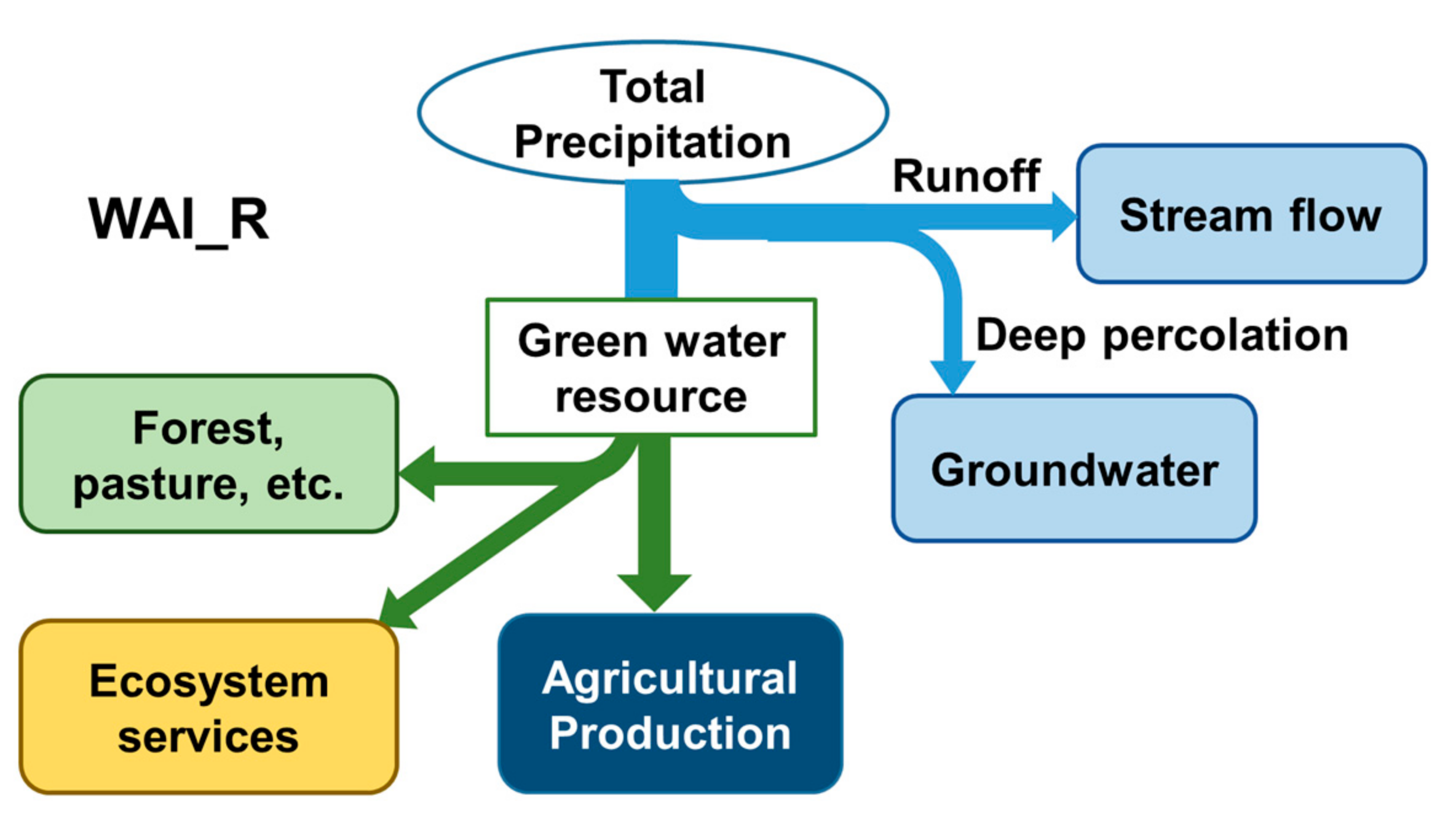
3. Method for Green Water Availability Assessment

A modified green water availability index (WAI_R) (Figure 1), which is an extension of the existing GWSI [16,19,31], was employed in this study. WAI_R is a metric that measures the fraction of green water resources, after the water demand of specified sectors (e.g., agriculture) is met by green water, available to all other remaining green water users (e.g., timber, pasture, ecosystem services). Like other area-based GWSI, WAI_R quantifies green water balance aggregated at a regional level (e.g., county). It does not consider green water availability at the field level. To estimate green water demand, we use total plant water demand rather than GWF. A companion green water WAI that uses GWF rather than crop water demand is also presented below (Equations (5) and (6)). For agricultural production, the green water resources used apply to all crops (rain-fed or irrigated). We assume that crop water demand will be met with green water resources first, and irrigation will be supplied only if there is a deficit in rainwater supply. In this sense, the application of irrigation water may affect yield but does not affect the portion of green water resources that would be available to other green water users. The WAI_R index proposed here is specifically designed to estimate the impacts of plant water demand on regional water resources (Figure 1). For available green water resources, Núñez et al. [19] use green water resources from existing cropland only; other studies consider all green water resources in a region, regardless of the land-use type [31,32]. In this study, we assume green water resources from all pervious land (e.g., cropland, pasture) are ultimately available for plant use; impervious land area (e.g., urban) and open water surfaces were excluded from green water resource calculations. We follow the suggestion of Liu et al. [18] to use annual green water resources, regardless of whether or not they are used by crops or other plants. Although some studies prefer to use growing season green water resources [19], off-season green water resources may be stored in soil or lost to deep percolation, depending on local soil and climate conditions. For instance, the portion of green water resources stored as soil moisture during the winter when the crop is dormant, which is also called carry-over soil moisture, can be used to meet the consumptive water needs of crops [70].
For a given county j, the fraction of green water resources needed to meet the demand from a certain sector i (WDI_Ri,j) is defined as the ratio of plant water demand from that sector to the total green water resources in county j (Equation (1)). Green water resources in a given county are defined as the volume of ER from all pervious land area in that county (Equation (1)). Pervious land area in county j (Apervious,j) is the total surface area in the county minus the total open water surface area, which includes streams, ponds, lakes, swamps and costal water area, and impervious (urban) area in that county (Equation (2)).
W D I _ R i , j   =   p l a n t   w a t e r   d e m a n d i , j g r e e n   w a t e r   r e s o u r c e j   =   p l a n t   w a t e r   d e m a n d i , j E R j × A p e r v i o u s , j
A p e r v i o u s , j   =   A t o t a l , j A w a t e r , j A i m p e r v i o u s , j
where: W D I _ R i , j   = the fraction of plant water demand of sector i in county j; ERj = annual effective rainfall depth (m/year) in county j; Atotal,j = total surface area (m2) of county j; Awater,j = open water surface area (e.g., river, ponds) (in m2) of county j; Aimpervious,j = impervious surface in urban area of county j (m2).
Once WDI_R is defined, WAI_R is simply calculated as the difference between 1 and WDI_R. Specifically, WAI_R is a general metric that can be applied to multiple sectors. Let S be a set of sectors, where sector i belongs to S, or i S .   Let WAI_Rnon i,j (Equation (3)) be the fraction of green water available for remaining sectors in S after meeting the needs of sector i, and let WAI_Rnon S,j (Equation (4)) be the fraction of green water resources available for remaining users after meeting the needs of all sectors in S. Then
W A I _ R n o n   i , j   =   1 W D I _ R i , j
W A I _ R n o n   S , j   =   1 W D I _ R S , j   =   1 i S W D I _ R i , j
where WAI_Rnon i,j = the fraction of green water available to the remaining sectors in S after meeting the needs of sector i; WAI_Rnon S,j = the fraction of green water available after meeting the needs of all sectors in S; WDI_RS,j = the fraction of green water resource needed to meet plant water needs of all sectors in S in county j.
The value of W A I _ R n o n   i , j or W A I _ R n o n   S , j   range from 0 to 1. A value of 1 means that 100% of the green water resources are available to sectors other than the specific sector(s). Take the agriculture sector as an example, a value of 1 means there is no agricultural production in a given region; a value of 0 means there are no remaining green water resources after meeting the demand from specified economic activities. When plant water demand exceeds supply, additional water resources (e.g., irrigation water) may be required to make up the green water deficit to sustain the growth. However, a detailed discussion on blue water consumption is outside the scope of this analysis. Although some studies (e.g., Quinteiro et al. [71]) have started to consider the dynamics between green and blue water in water scarcity footprint analysis, this study focuses on estimating green water availability.
In addition to WAI_R, we also calculated green water availability based on GWF for comparison. Similar to WAI_R, the fraction of green water resources consumed by a certain sector (WDI_R_Fi,j) is defined as the ratio of the GWF of sector i (in m3) to total green water resources (in m3) in county j (Equation (5)). Once WDI_R_F has been defined, the GWF-based green water availability index (WAI_R_F) can be defined as the difference between 1 and WDI_R_F (Equation (6)), as follows:
W D I _ R _ F i , j   =   W D I _ R _ F i , j   =   G W F i , j E R j × A p e r v i o u s , j
W A I _ R _ F n o n   i , j   =   1 W D I _ R _ F n o n   i , j
Similar to W A I _ R n o n   i , j , the value of W A I _ R _ F n o n   i , j also ranges from 0 to 1; a value of 0 means all green water resources consumed by sector i, and a value of 1 means the sector does not consume green water in region j.

3.1. Application to Agricultural Crop Production

The improved green water availability index (WAI_R) was applied to the production of three major crops (corn, soybeans and wheat) that represent the agriculture sector in the U.S. at the county level. We quantified the fraction of green water resources needed if the crop water demands of three crops in county j are met by green water (WDI_Rag,j) (Equation (7)), and the fraction of green water resources in county j that is available to remaining green water users (e.g., other crops, grassland, forest and ecosystem services) (WAI_Rnon_ag,j) (Equation (8)). The water demands of crop production can be calculated from crop evapotranspiration (ETc) and harvested acreages (Equation (7)):
W D I _ R a g , j   =   c E T c , j × A h a r v e s t , c , j E R j × A p e r v i o u s , j
W A I _ R n o n _ a g , j   =   1 W D I _ R a g , j
where: ETc,j = annual crop evapotranspiration depth (m/year) of crop c (corn, soybean, and wheat) in county j; and Aharvest,c,j = area (m2) of crop c harvested for all purposes in county j.
For comparison, we also applied the WAI_R_F metric to these three major crops. The fraction of green water resources consumed by the three crops ( W D I _ R _ F a g , j ) in county j is defined as the ratio of total crop green water consumption over green water resource in county j (Equation (9)). Green water availability for sectors other than these three crops ( W A I _ R _ F n o n _ a g , j ) is therefore the difference between 1 and W D I _ R _ F a g , j (Equation (10)):
W D I _ R _ F a g , j   =   c G W F c , j × A h a r v e s t , c , j E R j × A p e r v i o u s , j
W A I _ R _ F n o n _ a g , j   =   1 W D I _ R _ F a g , j
where GWFc,j = annual crop GWF in depth (m/year) of crop c in county j.

3.2. Crop Water Requirement and Green Water Footprint

Consumptive water use for individual crops (i.e., corn, soybeans, and winter and spring wheats) was quantified by estimating crop ET (ETc). For each crop, we estimated ETc as the product of reference ET (ETo) and crop coefficients (Kc) on a monthly basis at each county and summed to find annual crop ET [66]. Crop GWF was calculated as the minimum of crop water requirement (ETc) and green water resources (estimated from effective rain) on a monthly basis in each county and summed to find annual GWF. Monthly ETo was computed using the American Society of Civil Engineers’ (ASCE’s) standardized Penman-Monteith method [72]. Similar to previous studies [20,25], ET outside the crop growing season was not counted as crop water use in this analysis.
The growing period of winter wheat spans two consecutive years, but the calculation method is the same with corn and soybeans. This is because we used 30-year (1971–2000) mean monthly climate data, so whether a month is in year 1 or year 2 does not affect crop ET calculation. For instance, if winter wheat spans from October in year 1 to March in year 2, we simply calculated annual wheat ET by summing January–March ET and October–December ET.

3.3. Green Water Resource Estimation

Green water resources can be estimated from ER using several existing methods, including field monitoring, empirical equations, and soil water balance models [73]. A detailed review of ER estimation methods can be found in Dastane [34]. Many water footprint studies have utilized empirical equations to estimate ER [36,74,75]. Given the importance of ER in green water resource assessment, we employed three alternative ER estimation methods in this study to estimate 30-year (1971–2000) mean ER depth (mm/month) for each county in the conterminous U.S. at monthly intervals. Two are empirical methods, including the U.S. Department of Agriculture—Soil Conservation Service (USDA-SCS) (also known as Technical Release (TR)-21) method [70] and the Smith method [76]. The latter is a simplified version the USDA-SCS method implemented in the CROPWAT model [76]. The third method is derived from a water balance dataset (National Hydrography Dataset (NHD) Plus V2) [77].

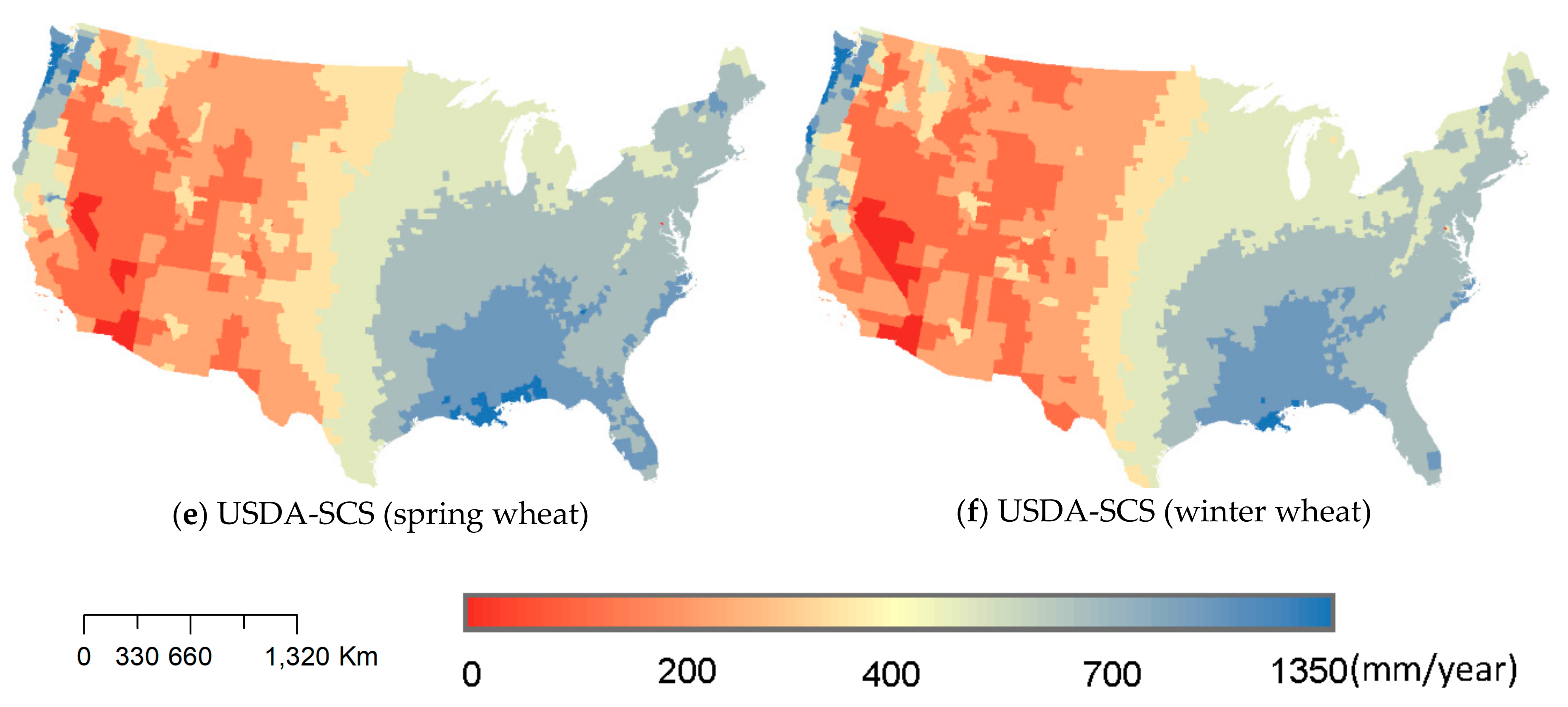
3.3.1. ER Based on the USDA-SCS Method

The USDA-SCS method [70] was developed with water balance calculations using 50 years of precipitation records at 22 locations throughout the U.S. The climate stations were selected to cover all climatic conditions across the 48 states in the continental U.S. Each of the stations has rainfall records of at least 25 years during the growing season of major crops. USDA scientists calculated daily soil water balance and related it to crop ET, precipitation, and soil water factors. Precipitation that is not lost to deep percolation or surface runoff is considered ER. The resulting equation for estimating effective rainfall is:
E R   =   S F × ( 0.70917 × P 0.82416 0.11556 ) ( 10 0.02426   ×   E T c )
And the soil factor (SF),
S F   =   ( 0.531747 + 0.295164 × D 0.057697 × D 2 + 0.003804 × D 3
where P is 30-year average monthly precipitation. ETc is average monthly crop evapotranspiration (inches). D is the “useable soil water storage” (inches), which is usually calculated as 40% to 60% of the available soil water capacity [35], depending on local irrigation practices. The management allowable soil water depletion for the three crops ranges from 50% to 65% [78]. In this study, we used 60% [75] because we assume farmers will use soil water first before applying irrigation water. However, using 50% or 60% does not make a noticeable difference in ER estimations; county level annual ER would decrease by 4.3% (SD = 2.46) if 50% is used. The soil water capacity layer was extracted from the Digital General Soil Map of the U.S. or STATSGO2 soil dataset [79].

3.3.2. ER Based on the Smith Method

The Smith method (Equation (13)), which is a simplification of the “USDA-SCS” method, assumes an average ET of 8 inches (≈203.2 mm) per month and a “useable” soil water storage of 3 inches (≈76.2 mm) [36]. The Smith method is more frequently used in the literature than the original USDA-SCS method [36,66,74,80], probably due to its simplicity and the wide application of the CROPWAT [78] model:
E R   =   { P × ( 125 0.2 × P ) 125 , f o r   P 250   m m / m o n t h 125 + 0.1 × P ,       f o r   P > 250   m m / m o n t h

3.3.3. ER Based on the NHDPlus V2 Data

The NHDPlus V2 dataset [77] provides simulated runoff at the catchment level, which is based on a soil water balance (WB) model developed by Wolock and MaCabe at USGS [81,82]. For this method, ER is the difference between precipitation (P) and runoff (RO) on a monthly basis (Equation (14)):
E R   =   P R O
where RO is model-simulated 30-year (1971–2000) average monthly runoff (mm/month), aggregated from original catchment level data using an area-weighting method. The weighting factors for a county that crossed the boundaries of multiple catchments were calculated separately based on the area of the county that fell inside each catchment and then aggregated to re-form the county-level mean runoff. The WB model uses monthly temperature and precipitation data to determine the proportions of monthly precipitation that are rain and snow [81,82]. Rainfall and melted snow contribute to runoff, which is calculated as the sum of direct runoff and surplus runoff, where direct runoff is computed from overland runoff. When soil moisture storage exceeds soil water capacity, the excess soil water contributes to runoff as surplus runoff [81,82]. Actual ET is equal to potential ET if rainfall and snow-melt exceed the potential ET. Soil moisture storage can be removed to support ET, but the fraction of moisture storage that can be removed decreases linearly with decreasing soil moisture [81,82]. This simplified scheme does not consider crop-specific ET. The WB model does not include a groundwater component, so deep percolation and base flow are not directly modeled.

3.3.4. Advantages and Limitations of the Three ER Estimation Methods

Among the three ER methods, the Smith method is the most convenient because it only requires monthly precipitation data; however, this method does not incorporate variations in local soil properties. The USDA-SCS method is conceptually more comprehensive because it includes a soil factor, but it still fails to account for soil water intake rates and rainfall intensity because of insufficient data and the complexity of these two factors [70]. In addition, although the USDA claimed that the 22 stations were selected to cover all climatic conditions in the U.S. [70], the USDA did not publish the data used for model development so the spatial and temporal pattern of the climate data is unclear. If climate and soil patterns of a given county are significantly different from those of the 22 stations, the USDA-SCS method may not work well. In addition, the experiments were published in 1970 and the 50 years of data reflect the period from the 1910s to the 1960s. Therefore, recent changes in soil infiltration rates caused by management practices (e.g., tillage) and rainfall intensity may require an update to the regression model published decades ago. In general, the USDA-SCS method is more applicable to regions with well-drained soil and low-intensity rainfall [34,73]. Unlike the two empirical approaches, the NHDPlus V2 dataset was derived from a WB model [81,82]. Although the model explicitly accounts for soil type and dynamics in water balance, it ignores the impact of plants and land management on runoff. In addition, the NHDPlus V2 dataset does not provide monthly changes in snow water storage, which means in areas with heavy snowfall it is difficult to differentiate runoff sourced from rainfall or snowmelt.

3.4. Study Area and Data Sources

Green water availability was analyzed at the county and regional level in the 48 continental states in the United States. We divided the 48 states into 10 major agricultural production regions (Figure 2) based on the boundaries of USDA farm production regions [83]. States within each region share similar farm production characteristics (e.g., crop types). Annual precipitation ranges from 100 to 3000 mm/year. Spatially, precipitation generally decreases from the southeastern U.S. to the western U.S., except in the northwestern costal area (Figure S1). Plantings of the major commodity crops (corn, soybeans, and wheat) are mostly concentrated in the Midwest (Figure 3) where soil is fertile and flat terrain is suitable for farming.
County-level corn, soybean, and wheat harvested acreages and yields in 2008 were collected from the USDA National Agricultural Statistics Service (NASS) (Table 2). The 30-year (1971–2000) mean monthly precipitation data at the county level were aggregated from the gridded Parameter-elevation Relationships on Independent Slopes Model (PRISM) dataset [84]. Ideally, the climate data period should cover the crop year (2008). However, the NHDPlus V2 dataset was based on 1971–2000 climate data and the potential ET (PET) data from the WATER model is only available for 1971–2000. To make sure that all methods use the same climate data, we used the 1971–2000 climate data for both ET and ER calculations. In fact, there is no significant change in precipitation patterns between the 1971–2000 and 1981–2010 PRISM datasets. For instance, county-level mean annual precipitation would decrease by 9.16 mm only (SD = 31.1) if 1981–2010 data is used. For the Smith and USDA-SCS methods, differences in annual ER calculated using the 1971–2000 versus 1981–2010 precipitation data are less than 10% for all but 24 counties.
Monthly potential ET and Crop coefficient (Kc) were provided by the WATER model [25,26,66] at the county and agricultural production region level, respectively (Table 2). Impervious land area and open water surface area (e.g., streams, lakes, swamps) for each county were extracted from the National Land Cover Database (NLCD) 2011 dataset [85] and the Cartographic Boundary Shapefiles [86], respectively.

4. Results and Discussion

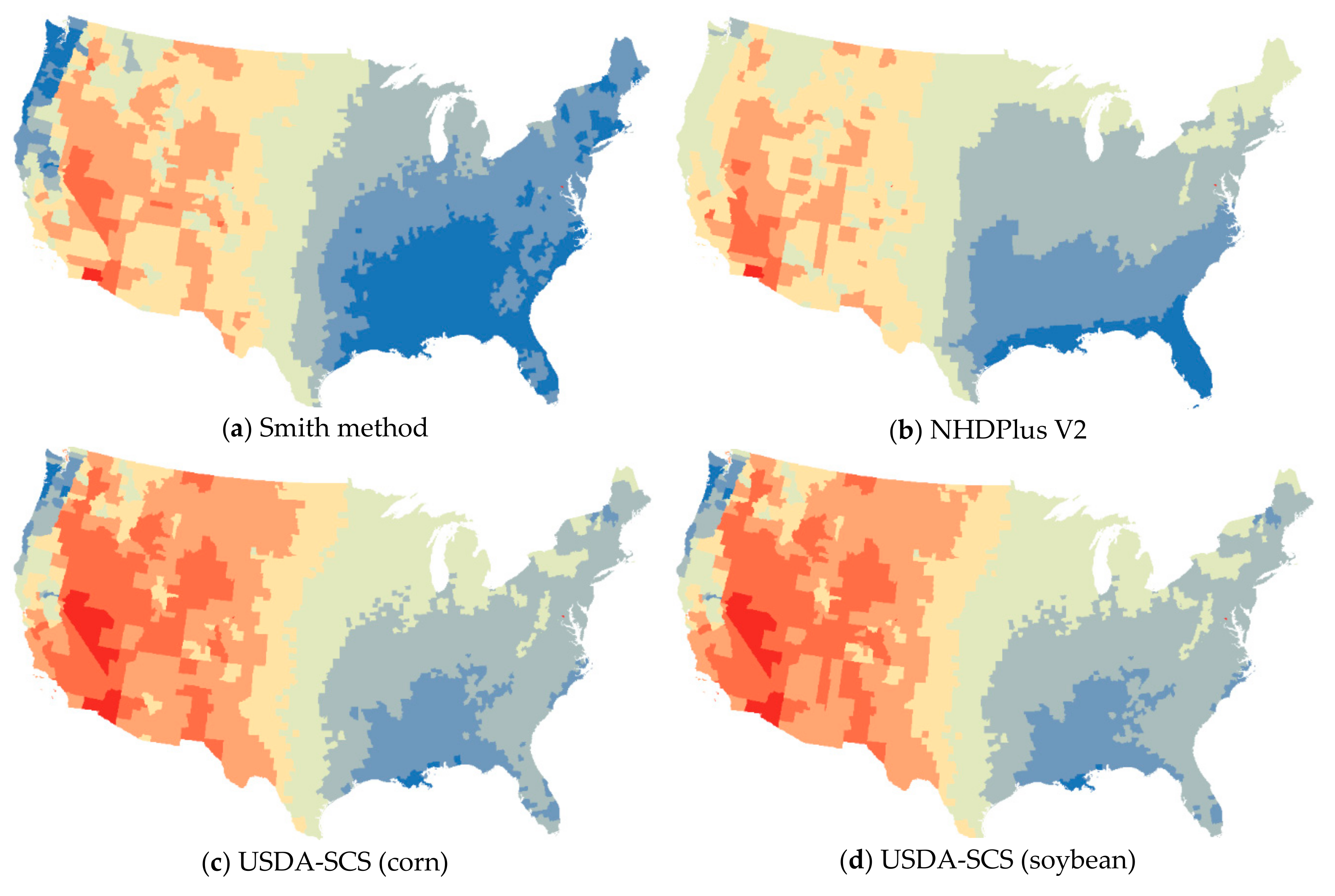
4.1. Comparison of Green Water Resources Estimated by Three Methods

Geospatially, all three green water resource estimations—based on the Smith method (ER_Smith), the USDA-SCS method (ER_USDA), and the NHDPlus (ER_NHD) method—presented a decreasing trend from the southeast region to the western states, except in the Pacific Northwest (Figure 4). This pattern largely follows the distribution pattern of annual precipitation (Figure S1). Among the three ER methods, ER_Smith (Figure 4a) and ER_USDA (Figure 4c–f) tend to have the highest and lowest values, and ER_NHD (Figure 4b) falls in the middle (Figure 4). In addition, discrepancies in annual ER estimations are more evident in the eastern U.S. than regions in the central and western U.S. Because the USDA-SCS method is crop specific, ER_USDA based on ETc of three major crops (i.e., corn, soybean, and wheat [including winter and spring wheat]) was also generated. The resulting four ER_USDA maps are quite similar (Figure 4c–f). This suggests that the USDA-SCS method for ER is consistent regardless of crop type.
In addition to spatial variation, the three green water resource estimates also presented diverse temporal patterns (Figure 5). For each agricultural production region, we plotted average monthly precipitation, ETc of corn, and three green water resource estimations, all weighted by county-level corn harvested acres (Figure 5). ETc of corn is presented as an example to illustrate that, depending on the region, peaks of green water supply and crop water demand could vary significantly. We plotted corn ETc only because it is the most widely planted commodity crop in the U.S. Still, using soybeans or wheat ETc generated very close results (not presented). Across the 10 regions, ER_Smith consistently produces higher results than ER_USDA. This is largely because the Smith method assumes an average monthly ETc of 200 mm throughout the year [37], which is much higher than the growing-season average monthly corn ETc (average = 117 mm/month, SD = 39.46) as determined by the Penman-Monteith equation that was used for ER_USDA calculation. For most regions, even peak corn ETc is less than 200 mm/month (Figure 5). On a monthly basis, the differences among the three estimations are generally smaller during the crop-growing seasons and higher during the non-growing seasons (Figure 5). Furthermore, months with peak corn ETc and ER_USDA values generally match each other, except in the Pacific and Southern Plains regions, where precipitation during crop-growing season is limited. The Smith method, on the other hand, correlates more closely with monthly precipitation. Although ER_Smith and ER_USDA generally follow monthly precipitation distributions, ER_NHD shows a more dynamic temporal pattern (Figure 5). This is because the ER_NHD also factors in changes in monthly snowmelt and soil water content, using a water balance model. However, monthly ER_NHD in the spring and fall needs to be interpreted cautiously for some regions. For instance, in areas with snowpack, ER_NHD may underestimate green water resources in the spring because runoff includes input from snowmelt, but monthly precipitation data does not track changes in snowpack. In the fall, ER_NHD diverges from precipitation in several regions (Figure 5) because the soil may have been saturated; thus additional precipitation input will be classified as runoff rather than green water resources.
Differences in temporal patterns suggest that agriculture and bioenergy production may use green water more effectively if land use composition matches the temporal green water resource distribution pattern better. Ideally, peaks of crop water demand would match with those of green water resources to minimize reliance on irrigation water, especially in regions with high blue water scarcity. For instance, effective rain in the Pacific region is relatively more abundant in the winter but very limited in the summer. In this case, growing winter wheat may use green water more effectively than growing corn. In addition, in counties with multiple crops and land uses, adjusting the fractions of land uses (e.g., cropland, forest, grassland) and crops with varying growing seasons or improving soil water management practices could be options. For example, the Delta region, while green water resources are limited in July and August, there are excessive green water resources in the spring and winter (Figure 5). Land management strategies like cover crops may be used to conserve more soil moisture and reduce the negative impacts of green water variability [88].
Few studies to date have verified alternative green water resource methods for a large study area, partly because a lack of field measurements at scale. Conceptually, the USDA-SCS and NHDPlus methods are more comprehensive, while the Smith method requires less input data. Wu et al. [66] found that the water footprints calculated based on the Smith method reasonably resemble peak monthly corn water use in the growing stage. A comparison study in the United Kingdom (U.K.) found that the Smith method turns out to be more accurate under U.K. conditions [36]. This is most likely because the USDA-SCS method was developed to fit U.S. conditions, while the Smith method was largely simplified for the ease of computation. For the NHDPlus method, interpreting results for spring in certain regions may be difficult. In short, considerable uncertainties remain in green water resource estimates. For county-level green water availability analysis, WAI_R was primarily calculated based on the Smith method, so the method for estimating crop water demand and green water footprint from this study would be consistent with our previous studies [25,26,66].

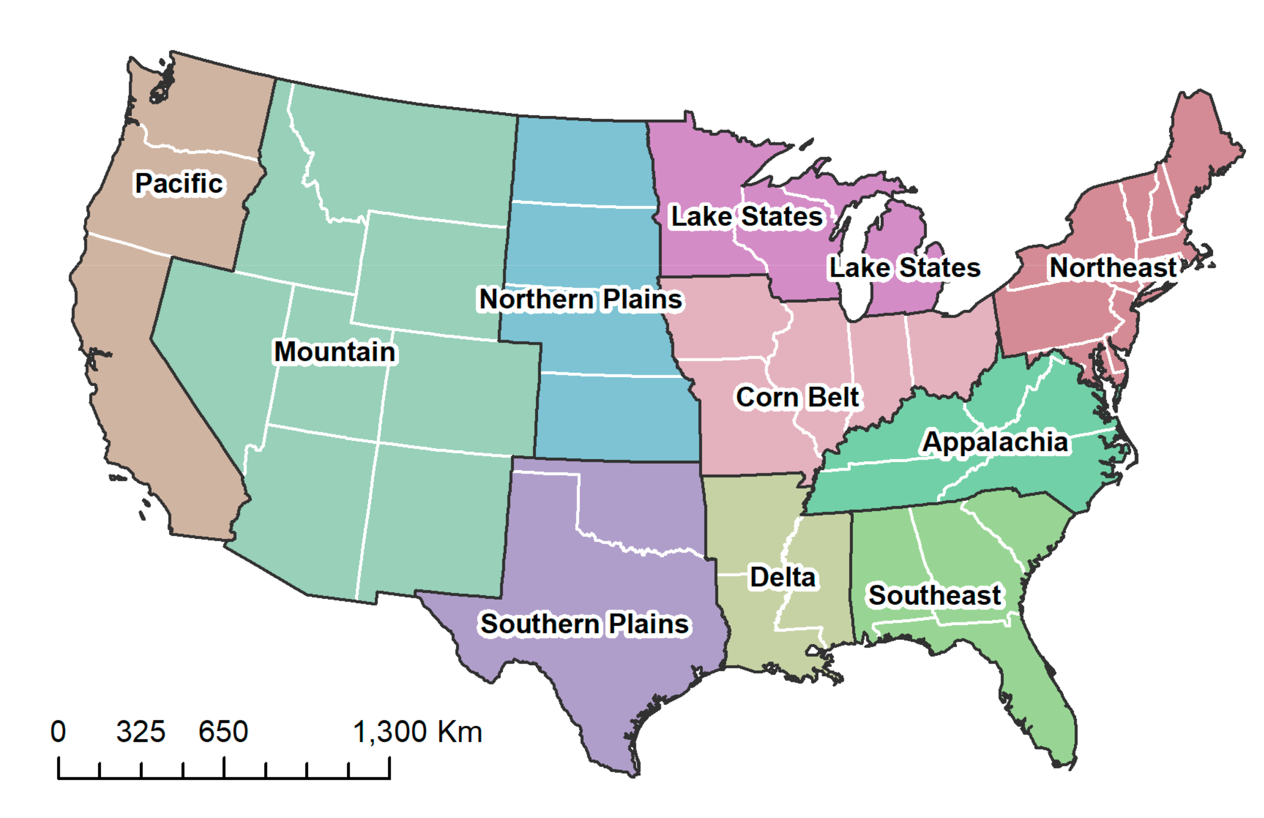
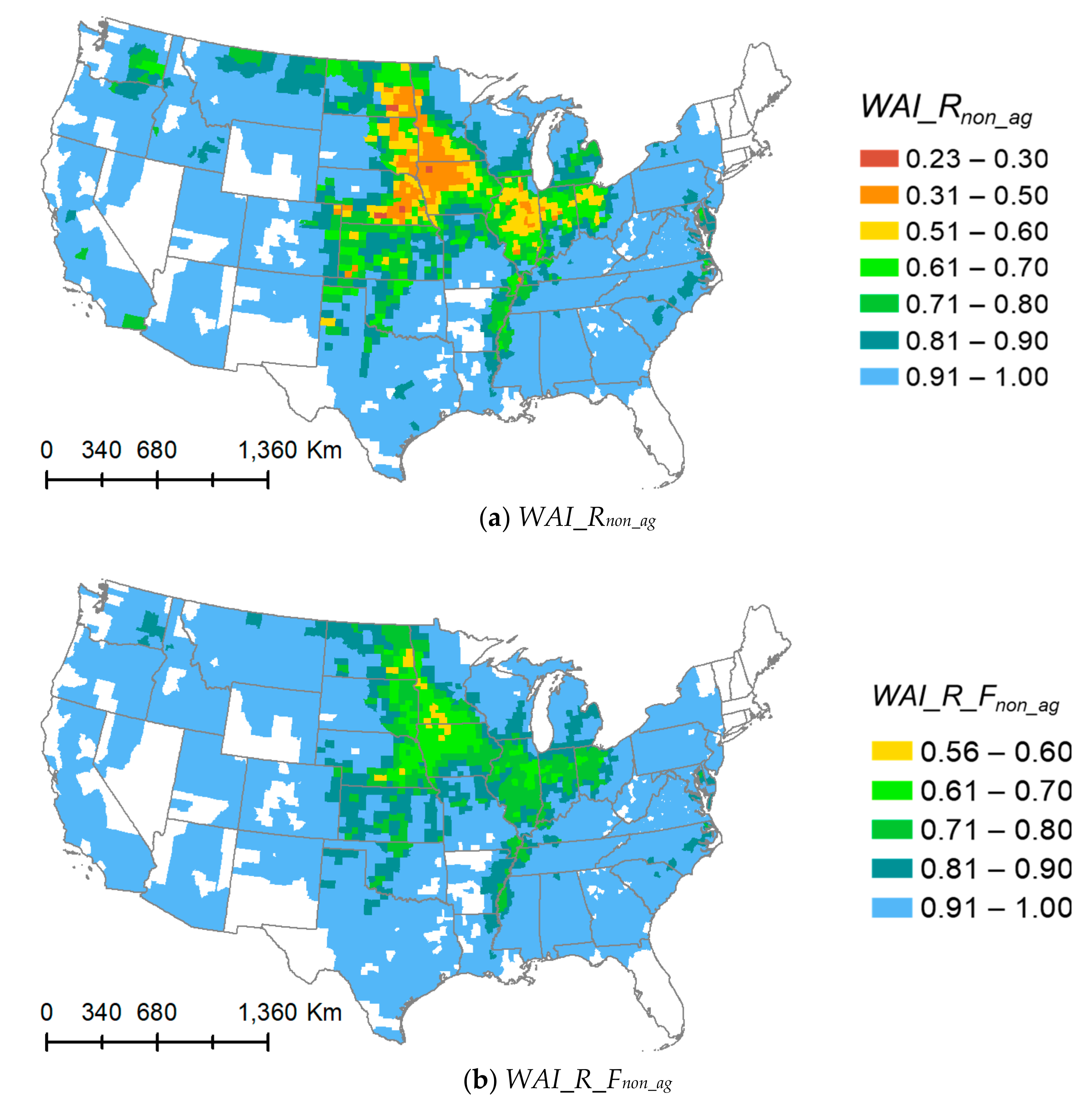
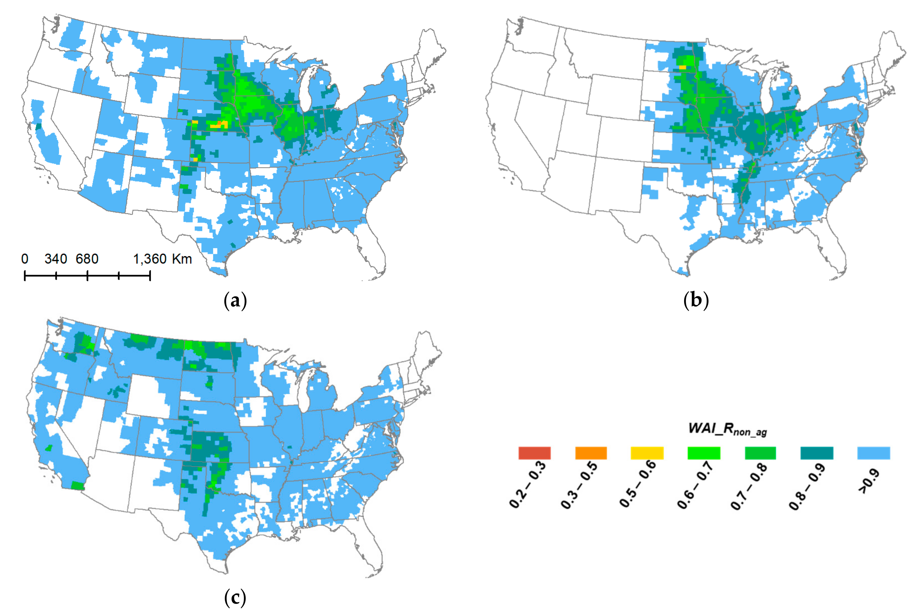
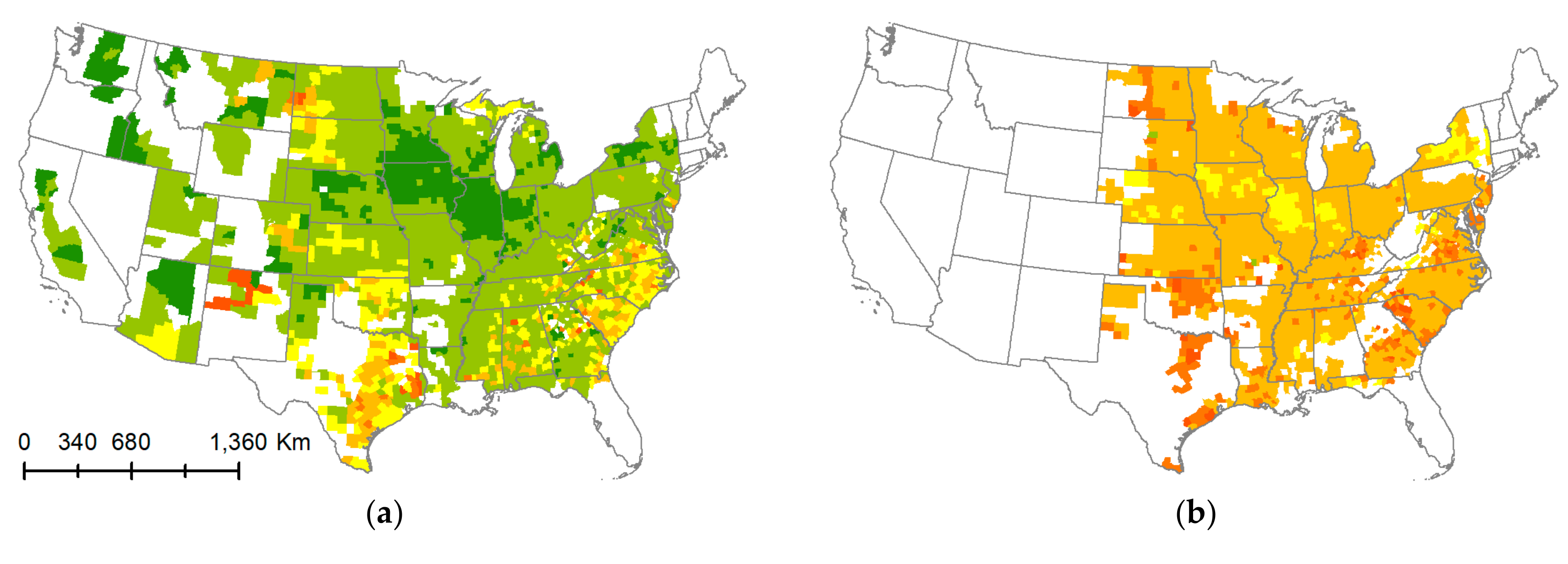
4.2. Regional and County-Level Green Water Availability

Using the WAI_R and WAI_R_F metrics, a regional and county-level green water availability analysis was applied to three major commodity crops (corn, soybean, and wheat) in the conterminous United States. The two metrics quantified the impacts of crop water demand and crop GWF on green water availability to all other remaining economic activities (e.g., other crops, grassland, and forest) and ecosystem services. These fractions reflect green water balance aggregated at the county or regional level, disregarding green water availability at the field scale. In this sense, the area-based analysis demonstrated how current land use composition and potential land use change (e.g., expansion of rain-fed cropland) may affect green water availability.
WAI_Rnon_ag and WAI_R_Fnon_ag values suggest that crop production overall uses less than 30% of annual green water resources at the agricultural production region level, but substantial spatial variation exists at the county level (Table 3 and Figure 6). For the 10 agricultural production regions, WAI_Rnon_ag and WAI_R_Fnon_ag ranged from 0.71 to 0.98 and from 0.82 to 0.99, respectively (Table 3). At the county level, WAI_Rnon_ag (Figure 6a) and WAI_R_Fnon_ag (Figure 6b) ranged from 0.23 to 1.0 and from 0.56 to 1.0, respectively. Among the 2694 counties with major crop production in 2008, there are about five counties with high (WAI_Rnon_ag < 0.3) and 106 counties with medium (0.3 < WAI_Rnon_ag < 0.5) tensions between crop water demand and green water resource (Table 4). When measured by WAI_R_Fnon_ag, there are about 155 counties with moderately low green water availability (0.5 < WAI_R_Fnon_ag < 0.7) (Table 5). Overall, counties facing moderate or higher green water resource tensions are mostly located in Iowa, Illinois, Minnesota, Nebraska, and South Dakota (Figure 6). The WAI_R_Fnon_ag values are significantly higher than WAI_Rnon_ag in several regions because WAI_R_Fnon_ag is calculated based on GWF rather than crop water demand, since GWF can be significantly lower than crop water demand if precipitation is limited during crop-growing season. In this case, WAI_Rnon_ag and WAI_R_Fnon_ag can be complementary to each other. WAI_Rnon_ag could reflect the tension between crop water demand and green water resources better when green water consumption is limited by supply of green water resources, however, WAI_R_Fnon_ag provides the actual amount of green water resources available to other sectors.
County-level green water available to each economic sector in a region depends on both green water resources and crop water use in that county. Although annual precipitation is relatively abundant in the Corn Belt, high crop acreages drive down green water availability substantially in this region. For reference, we also present regional crop water demand (CWD), expressed as intensity or the annual volume of rainwater needed per volume of crop produced (in dry short tons, d.s.t, which is equivalent to 0.907 metric ton of dry biomass) (Figure 7). Results clearly indicate that CWDs for all three major crops in the Midwest are among the lowest in the U.S. (Figure 7), which means there is higher water use efficiency in this region, and is consistent with previous studies [22,89]. CWDs in the Northern Plains, which is the second largest crop production region in the U.S., are moderately higher —41%, 22%, and 17% for corn, soybean, and wheat, respectively—than in the Corn Belt. CWDs in the Southern Plains for soybean and wheat are much greater than in the Midwest. These differences in regional CWDs can be attributed to spatial variability in soil and climate conditions, as well as agricultural managing practices. Other variables like crop varieties also affect crop water demand and consumption.

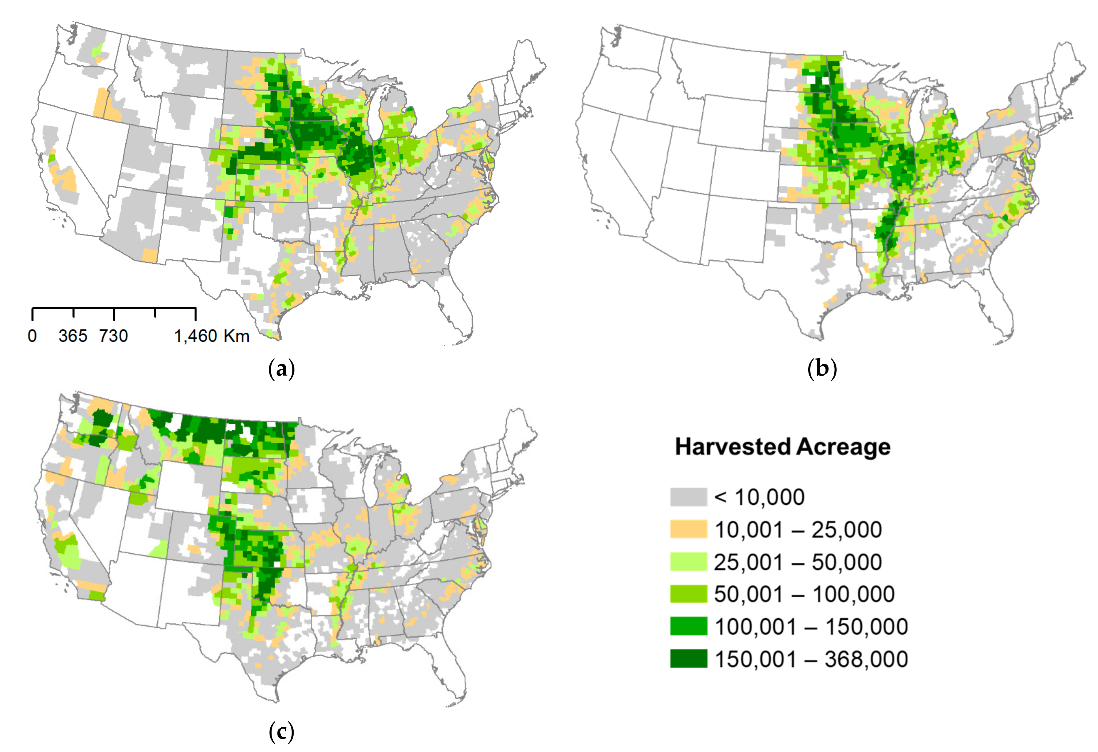
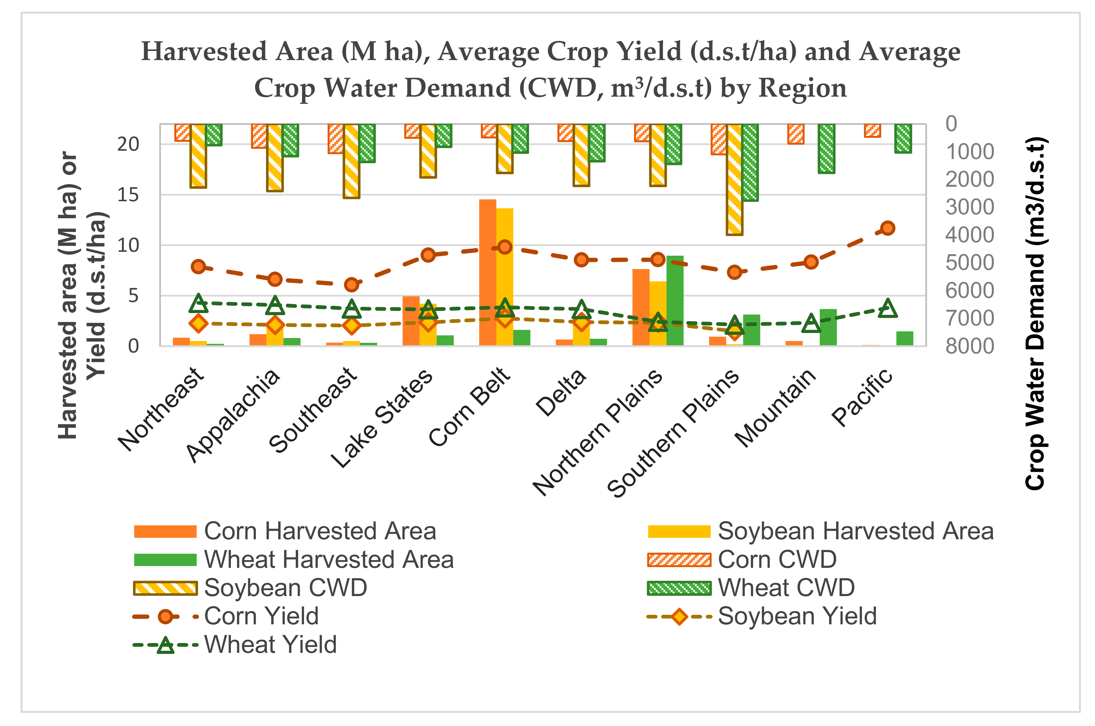
4.3. Green Water Availability by Crop Type

Compared to green water resource distribution (Figure 4), variations in local WAI_Rnon_ag and WAI_R_Fnon_ag strongly correlate to and are thus impacted by the spatial distribution of harvested crop acres (Figure 3 and Figure 6). County-level WAI_Rnon_ag is often dominated by the water demands of different crops. This pattern is clearly demonstrated by crop-specific WAI_Rnon_ag (Figure 8) values, which measure the fraction of green water resources available for other uses after meeting crop water demand of a specific crop (e.g., corn). In the Midwest, corn and soybean acreages contribute the most to the volume of crop water demand (Figure 8a,b). Although wheat plays an important role in certain areas (e.g., Montana), total wheat acres are much less than corn and soybean acres in most areas.
The spatial pattern of crop-specific WAI_Rnon_ag does not mean crops in the Midwest use more water on a per-unit biomass basis. In fact, county-level CWD (m3/d.s.t) of the three crops (Figure 9) clearly indicate that counties in the Corn Belt are more water efficient than other areas. In addition, it seems that some counties located in northwestern states (Washington, Portland, Idaho, Oregon) are also water efficient in terms of corn and wheat production. Relatively low WAI_Rnon_ag values in these counties suggest it would be possible to increase crop acreages in these counties from a green water resource perspective, but land-use changes may cause other problems (e.g., deforestation).

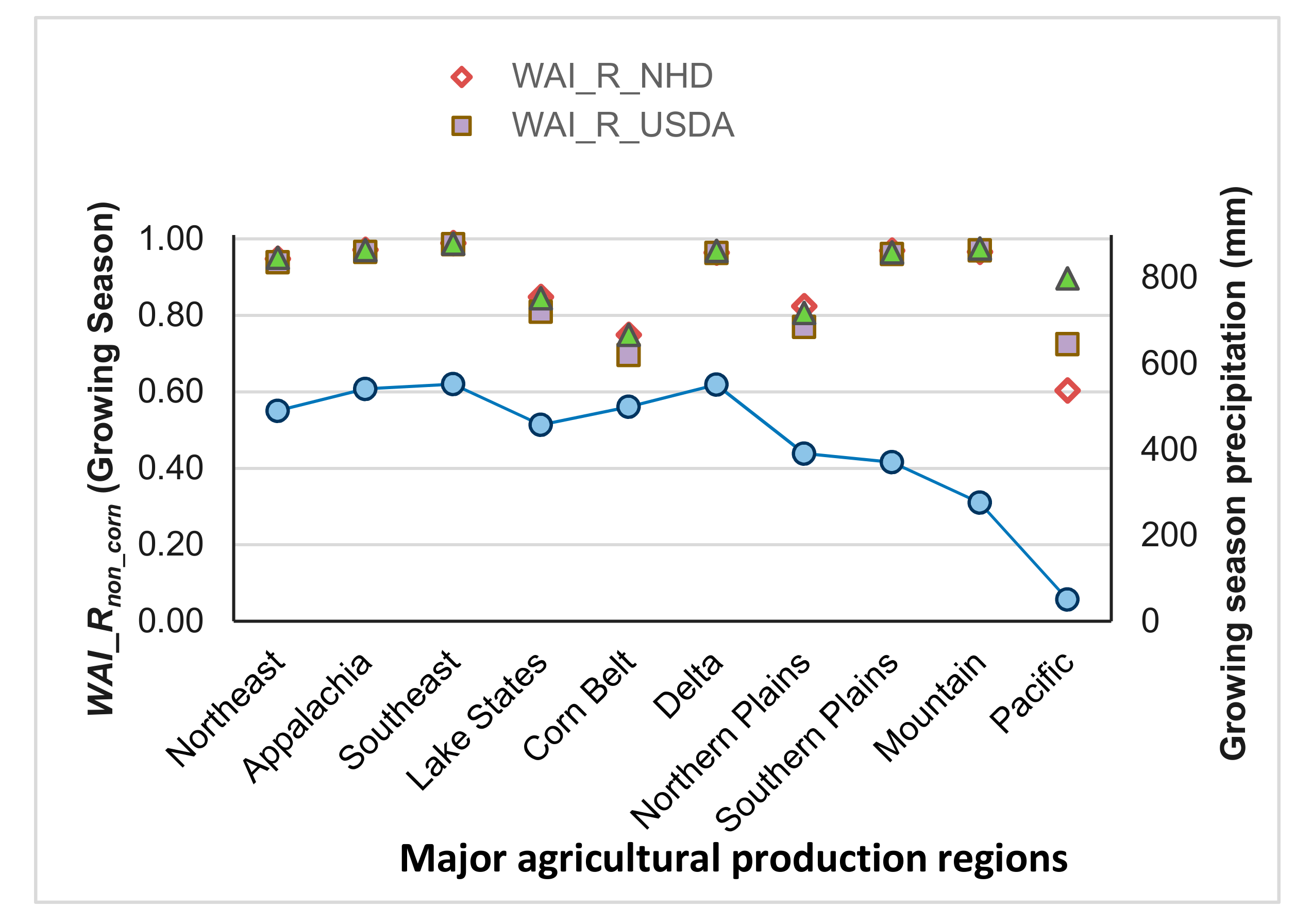
4.4. Annual Versus Growing Season Green Water Availability

Depending on local soil and climate conditions, off-season green water resources may lost to the atmosphere or contribute to blue water storage via deep percolation. In this case, it is helpful to estimate the green water resources available during the crop-growing season only if green water meets all crop water demand. Given that corn is the most widely produced commodity crop in the U.S., we also present the regional WAI_R based on growing season green water resources and of corn (WAI_Rnon_corn) (Figure 10) as an example to illustrate how the temporal boundary of green water resources may affect the estimation of green water availability. Specifically, the WAI_Rnon_corn metric describes that, if all corn water demand met by green water, the fraction of green water resources are available to all other remaining green water users, aggregated at the county level. Results indicated that, when the green water resource is limited to the growing season only, total corn water demand alone would drive down green water availability substantially. A low WAI_Rnon_corn value means less green water available for other crops and plants in the region. Because of extremely low growing season precipitation, WAI_Rnon_corn in the Pacific could fall to 0.9 (Figure 10, Smith method) from an annual based WAI_R of 0.98 (Figure 8a). Growing-season WAI_Rnon_corn for the Corn Belt, Lake States, and Northern Plains would decrease 0.12, 0.06 and 0.07, respectively, compared with the annual-based index (Figure 8a).
Results in annual versus growing-season-based WAI_R values suggest that green water availability assessments can be sensitive to the temporal boundary of WAI_R analysis. In addition, it is important to note that the growing-season WAI_R could be conservative in certain soil conditions, because crops may utilize some of the non-growing season green water resource stored in the soil. Although field monitoring through sensor technology has been developed to guide precision agriculture programs and practices, it would be helpful if a national consistent soil water dynamic database could be developed for the U.S. in future studies.

4.5. Implications of Regional Water Resource Management for Bioenergy Production

Several regions produce the three major crops for feed, food, fiber, and fuel. To evaluate the impact of bioenergy feedstock production on green water availability, demand from the production of food, feed, and fiber is excluded. The resulting WAI_R metric—WAI_Rnon_bioenergy—describes the green water resources available for other uses if the water demand of biofuel feedstock production is met by green water resources only. For all but 149 counties (mostly located in Iowa, Nebraska, Minnesota, and Illinois), more than 90% of rainwater is still available to non-bioenergy productions (Figure 11). A majority of the 149 counties with WAI_Rnon_bioenergy values of 0.8–0.9, are concentrated in Iowa and Nebraska. If 24% of corn stover and 30% of wheat straw were also harvested as cellulosic biofuel feedstock [26,68] in 2008, holding total harvested crop acres and climate conditions constant, then regional mean WAI_Rnon_bioenergy would decrease slightly (0.03–0.05) for agricultural production regions in the Midwest, but WAI_Rnon_bioenergy would still be higher than 0.8 for all counties in these regions. These results suggest attributes of cellulosic feedstock to regional green water availability are small under the 2008 scenario.
From the perspective of water resource management, the production of the three major crops is most water efficient in the Corn Belt and Lake States because of their low CWD (Figure 7) and relatively abundant green water resources (Figure 4). Low green water availability for non-agriculture sectors in the Corn Belt is driven by food and feed production, with minimal contributions from biofuel feedstock production (Figure 11). However, when the production of food, fuel, feed, and fibers and the green water use by forestry and ecosystems are all accounted for, the aggregate impact on green water resource availability could become substantial. Therefore, it is critical to consider green water demands from multiple sectors when planning regional development.

4.6. Limitations and Future Work

The green water availability assessment approach presented in this study is applicable for large-scale assessments at varying spatial scales (e.g., watershed, state, and national). However, uncertainties exist, mainly associated with crop water demand calculation and green water resource estimations, due to incomplete data sources and assumptions made in estimation methods. County-level crop coefficients (Kc) for corn, soybean, and wheat are required in ET calculations, but are incomplete for all major crops. Therefore, we adopted regionalized crop coefficients for the 10 agricultural resource regions, but this practice may overlook variations in Kc within regions. In addition, monthly potential ET (ETo) was computed using the ASCE’s standardized Penman-Monteith method only. Although this is the dominant method used in the United States [26], other ET estimation methods exist and the uncertainties related to ET estimation by using different methods could be quite significant, especially in areas with high rainfall [90]. Finally, effective rain plays a central role in determining green water resources, and WAI_R based on varying temporal boundaries (annual vs. growing season) can lead to very different results for certain regions.
In this study, green water resources were quantified from effective rain using three alternative methods. The choice of effective rain methodology affects the spatial and temporal distribution patterns and the intensity of green water resources, the variation of which increases with increasing geospatial resolution. For future study, analyzing green water availability and competition on a monthly basis would be helpful for certain crops. However, determining monthly green water resources is more complicated than simply calculating monthly effective rain and crop water use, because green water resources can be stored in soil as carryover moisture. In this sense, a monthly analysis would require an integrated metric or framework that simultaneously considers the interactions among crop water use, soil moisture dynamics, and irrigation applications.

5. Conclusions

Although green water is vital for agricultural production and the terrestrial ecosystem, previous water resource assessments often focus on blue water. In this study, we present a first estimation of county-based green water availability, by applying a modified water availability index (WAI_R) to major crop (e.g., corn, soybeans, and wheat) production in the United States. The WAI_R metric was employed to quantify the fraction of green water resources available to non-agriculture sectors (e.g., grassland, forest, ecosystem services), assuming all crop water demands are met by green water. The metric quantifies green water balances aggregated at the county and farm production region level, disregarding green water availability at a field or land-use level. For comparison, a WAI (WAI_R_F) based on green water footprint was also presented, which quantifies the fraction of green water resources actually available to other users after accounting for the green water consumption of three crops.
Results highlight the spatial heterogeneity and temporal complexity of green water resources, as well as the heavy reliance of agriculture production on green water resources in the United States. In 2008, regional level mean WAI_Rnon_ag and WAI_R_Fnon_ag ranged from 0.71 to 0.98 and from 0.82 to 0.99, respectively. At the county level, however, fresh water was significantly constrained in five counties with a WAI_Rnon_ag value of lower than 0.3, which translates to a 70% demand for green water resources by the three crops. When measured by WAI_R_Fnon_ag, there are 17 counties with a values lower than 0.6, which means the three crops consumed more than 40% of annual green water resources in those counties. Geospatially, WAI_Rnon_ag and WAI_R_Fnon_ag are relatively higher in the Midwest, because of large crop acreages that are responsible for producing about 82% of the crops for the nation. However, crop production is also water efficient in this region, because water use per dry ton of biomass produced in the region is among the lowest across the 10 farm production regions. Seasonal analysis further revealed a substantial variability of crop water deficits during the growing season across regions, especially in Pacific west, which limits sustainable production of rain-fed crops. For areas with limited seasonal green water resources, adjusting land-use types to match seasons of high plant water demand with peaks of green water supply could be an option to use green water more effectively. In addition, improving soil water management strategies (e.g., adoption of cover crops) to increase carry-over soil moisture may also help with mitigating the negative impacts of seasonal variations in green water supply.
The development and scale-up of any land-based biomass production needs to be analyzed from the perspectives of resource availability and sustainability. Although surface (irrigation) water constraints have been stressed repeatedly, green water was usually taken for granted. Findings based on 2008 data suggest that bioenergy feedstock production demands a relatively small fraction of green water resources, but future large-scale biofuel feedstock production may substantially change land use composition (e.g., increase in woody crops for bioenergy), and therefore plant water consumption, in major agricultural regions [26]. To reduce competing use of surface and ground water (blue water consumption), rain-fed energy crops or biomass production is preferred in the bioenergy development in the U.S. In this case, availability of green water resources for large-scale feedstock production should be carefully evaluated. For agriculture and bioenergy production, the analysis presented can help decision makers consider geographical variations in green water availability when planning land-based biomass production sites, types, and production scales. However, analysis of green water availability alone is not sufficient for sustainable water management. Future studies should consider integrating green-blue water availability with land use at large scale, because land use patterns are likely to impact both blue and green flows.

Disclaimer

The submitted manuscript has been created by UChicago Argonne, LLC, Operator of Argonne National Laboratory (“Argonne”). Argonne, a U.S. Department of Energy Office of Science laboratory, is operated under Contract No. DE-AC02-06CH11357. The U.S. Government retains for itself, and others acting on its behalf, a paid-up nonexclusive, irrevocable worldwide license in said article to reproduce, prepare derivative works, distribute copies to the public, and perform publicly and display publicly, by or on behalf of the Government. The Department of Energy will provide public access to these results of federally sponsored research in accordance with the DOE Public Access Plan. http://energy.gov/downloads/doe-public-accessplan

Supplementary Materials

Figure S1: County-level 30-year (1971–2000) average annual precipitation for the conterminous United States.

Acknowledgments

This work was made possible by funding from the U.S. Department of Energy, Office of Energy Efficiency and Renewable Energy, Bioenergy Technologies Office (BETO), under contract #DE-AC02-06CH11357. We would like to thank Kristen Johnson of BETO for her valuable input and suggestions throughout the study. The authors are grateful to the three anonymous reviewers for their constructive suggestions.

Author Contributions

May Wu initiated project and directed analysis; Hui Xu performed the analysis; Hui Xu and May Wu analyzed the data; Hui Xu wrote the paper.

Conflicts of Interest

The authors declare no conflict of interest and the founding sponsors had no role in the design of the study; in the collection, analyses, or interpretation of data; in the writing of the manuscript; or in the decision to publish the results.

References

  1. Vörösmarty, C.J.; McIntyre, P.B.; Gessner, M.O.; Dudgeon, D.; Prusevich, A.; Green, P.; Glidden, S.; Bunn, S.E.; Sullivan, C.A.; Liermann, C.R.; et al. Global threats to human water security and river biodiversity. Nature 2010, 467, 555–561. [Google Scholar] [CrossRef] [PubMed]
  2. Rockström, J.; Steffen, W.; Noone, K.; Persson, A.; Chapin, F.S.; Lambin, E.F.; Lenton, T.M.; Scheffer, M.; Folke, C.; Schellnhuber, H.J.; et al. A safe operating space for humanity. Nature 2009, 461, 472–475. [Google Scholar] [CrossRef] [PubMed]
  3. Gerten, D.; Hoff, H.; Rockström, J.; Jägermeyr, J.; Kummu, M.; Pastor, A.V. Towards a revised planetary boundary for consumptive freshwater use: Role of environmental flow requirements. Curr. Opin. Environ. Sustain. 2013, 5, 551–558. [Google Scholar] [CrossRef]
  4. Mekonnen, M.M.; Hoekstra, A.Y. Four billion people facing severe water scarcity. Sci. Adv. 2016, 2, e1500323. [Google Scholar] [CrossRef] [PubMed]
  5. Kummu, M.; Guillaume, J.H.A.; de Moel, H.; Eisner, S.; Flörke, M.; Porkka, M.; Siebert, S.; Veldkamp, T.I.E.; Ward, P.J. The world’s road to water scarcity: Shortage and stress in the 20th century and pathways towards sustainability. Sci. Rep. 2016, 6, 38495. [Google Scholar] [CrossRef] [PubMed]
  6. Falkenmark, M. Growing water scarcity in agriculture: Future challenge to global water security. Philos. Trans. R. Soc. A Math. Phys. Eng. Sci. 2013, 371, 20120410. [Google Scholar] [CrossRef] [PubMed]
  7. Averyt, K.; Meldrum, J.; Caldwell, P.; Sun, G.; McNulty, S.; Huber-Lee, A.; Madden, N. Sectoral contributions to surface water stress in the coterminous United States. Environ. Res. Lett. 2013, 8, 35046. [Google Scholar] [CrossRef]
  8. Gerten, D.; Heinke, J.; Hoff, H.; Biemans, H.; Fader, M.; Waha, K. Global Water Availability and Requirements for Future Food Production. J. Hydrometeorol. 2011, 12, 885–899. [Google Scholar] [CrossRef]
  9. USGS (U.S. Geological Survey). WaterWatch. Available online: https://waterwatch.usgs.gov/new/index.php?id=ww_past (accessed on 16 July 2017).
  10. US Census Bureau Census. 2010. Available online: http://quickfacts.census.gov/qfd/states/13/13135.html (accessed on 16 May 2015).
  11. Moore, B.C.; Coleman, A.M.; Wigmosta, M.S.; Skaggs, R.L.; Venteris, E.R. A high spatiotemporal assessment of consumptive water use and water scarcity in the conterminous United States. Water Resour. Manag. 2015, 29, 5185–5200. [Google Scholar] [CrossRef]
  12. Roy, S.B.; Chen, L.; Girvetz, E.H.; Maurer, E.P.; Mills, W.B.; Grieb, T.M. Projecting water withdrawal and supply for future decades in the U.S. under climate change scenarios. Environ. Sci. Technol. 2012, 46, 2545–2556. [Google Scholar] [CrossRef] [PubMed]
  13. Tidwell, V.C.; Moreland, B.D.; Zemlick, K.M.; Roberts, B.L.; Passell, H.D.; Jensen, D.; Forsgren, C.; Sehlke, G.; Cook, M.A.; King, C.W.; et al. Mapping water availability, projected use and cost in the western United States. Environ. Res. Lett. 2014, 9, 64009. [Google Scholar] [CrossRef]
  14. Sun, G.; Mcnulty, S.G.; Myers, J.A.M.; Cohen, E.C. Impacts of Climate Change, Population Growth, Land Use Change, and Groundwater Availability on Water Supply and Demand across the Conterminous U.S. Water Supply 2008, 6, 1–30. [Google Scholar]
  15. Caldwell, P.V.; Sun, G.; McNulty, S.G.; Cohen, E.C.; Moore Myers, J.A. Impacts of impervious cover, water withdrawals, and climate change on river flows in the conterminous US. Hydrol. Earth Syst. Sci. 2012, 16, 2839–2857. [Google Scholar] [CrossRef] [Green Version]
  16. Hoekstra, A.Y.; Chapagain, A.K.; Aldaya, M.M.; Mekonnen, M.M. The Water Footprint Assessment Manual; Earthscan: London, UK, 2011; ISBN 9781849712798. [Google Scholar]
  17. Falkenmark, M.; Rockström, J. The New Blue and Green Water Paradigm: Breaking New Ground for Water Resources Planning and Management. J. Water Resour. Plan. Manag. 2006, 132, 129–132. [Google Scholar] [CrossRef]
  18. Liu, J.; Yang, H.; Gosling, S.N.; Kummu, M.; Flörke, M.; Pfister, S.; Hanasaki, N.; Wada, Y.; Zhang, X.; Zheng, C.; et al. Water scarcity assessments in the past, present, and future. Earth’s Future 2017, 5, 545–559. [Google Scholar] [CrossRef]
  19. Núñez, M.; Pfister, S.; Antón, A.; Muñoz, P.; Hellweg, S.; Koehler, A.; Rieradevall, J. Assessing the Environmental Impact of Water Consumption by Energy Crops Grown in Spain. J. Ind. Ecol. 2013, 17, 90–102. [Google Scholar] [CrossRef]
  20. Liu, J.; Zehnder, A.J.B.; Yang, H. Global consumptive water use for crop production: The importance of green water and virtual water. Water Resour. Res. 2009, 45. [Google Scholar] [CrossRef]
  21. Mekonnen, M.M.; Hoekstra, A.Y. The green, blue and grey water footprint of crops and derived crop products. Hydrol. Earth Syst. Sci. 2011, 8, 1577–1600. [Google Scholar] [CrossRef] [Green Version]
  22. White, M.; Gambone, M.; Yen, H.; Arnold, J.; Harmel, D.; Santhi, C.; Haney, R. Regional Blue and Green Water Balances and Use by Selected Crops in the U.S. J. Am. Water Resour. Assoc. 2015, 51, 1626–1642. [Google Scholar] [CrossRef]
  23. Senay, G.B.; Friedrichs, M.; Singh, R.K.; Velpuri, N.M. Evaluating Landsat 8 evapotranspiration for water use mapping in the Colorado River Basin. Remote Sens. Environ. 2016, 185, 171–185. [Google Scholar] [CrossRef]
  24. Gerbens-Leenes, P.W.; van Lienden, A.R.; Hoekstra, A.Y.; van der Meer, T.H. Biofuel scenarios in a water perspective: The global blue and green water footprint of road transport in 2030. Glob. Environ. Chang. 2012, 22, 764–775. [Google Scholar] [CrossRef]
  25. Chiu, Y.W.; Wu, M. Assessing county-level water footprints of different cellulosic-biofuel feedstock pathways. Environ. Sci. Technol. 2012, 46, 9155–9162. [Google Scholar] [CrossRef] [PubMed]
  26. Wu, M.; Ha, M. Water Consumption Footprint of Producing Agriculture and Forestry Feedstocks, Chapter 8, 2016 Billion-Ton Report, Volume 2: Environmental Sustainability Effects of Select Scenarios from Volume 1; Department of Energy Office of Energy Efficiency & Renewable Energy: Washington, DC, USA, 2017. [Google Scholar]
  27. Núñez, M.; Pfister, S.; Roux, P.; Antón, A. Estimating water consumption of potential natural vegetation on global dry lands: Building an LCA framework for green water flows. Environ. Sci. Technol. 2013, 47, 12258–12265. [Google Scholar] [CrossRef] [PubMed]
  28. Quinteiro, P.; Dias, A.C.; Silva, M.; Ridoutt, B.G.; Arroja, L. A contribution to the environmental impact assessment of green water flows. J. Clean. Prod. 2015, 93, 318–329. [Google Scholar] [CrossRef]
  29. Lathuillière, M.J.; Bulle, C.; Johnson, M.S. Land Use in LCA: Including Regionally Altered Precipitation to Quantify Ecosystem Damage. Environ. Sci. Technol. 2016, 50, 11769–11778. [Google Scholar] [CrossRef] [PubMed]
  30. Boulay, A.-M.; Hoekstra, A.Y.; Vionnet, S. Complementarities of Water-Focused Life Cycle Assessment and Water Footprint Assessment. Environ. Sci. Technol. 2013, 47, 11926–11927. [Google Scholar] [CrossRef] [PubMed]
  31. Rodrigues, D.B.B.; Gupta, H.V.; Mendiondo, E.M. A blue/green water-based accounting framework for assessment of water security. Water Resour. Res. 2014, 50, 7187–7205. [Google Scholar] [CrossRef]
  32. Veettil, A.V.; Mishra, A.K. Water security assessment using blue and green water footprint concepts. J. Hydrol. 2016, 542, 589–602. [Google Scholar] [CrossRef]
  33. Vanham, D.; Hoekstra, A.Y.; Wada, Y.; Bouraoui, F.; de Roo, A.; Mekonnen, M.M.; van de Bund, W.J.; Batelaan, O.; Pavelic, P.; Bastiaanssen, W.G.M.; et al. Physical water scarcity metrics for monitoring progress towards SDG target 6.4: An evaluation of indicator 6.4.2 “Level of water stress.”. Sci. Total Environ. 2018, 613, 218–232. [Google Scholar] [CrossRef] [PubMed]
  34. Dastane, N.G. Effective rainfall in irrigated agriculture. In Irrigation and Drainage Paper No. 25; Food and Agriculture Organization of the United Nations: Rome, Italy, 1974. [Google Scholar]
  35. USDA Soil Conservation Serivce. Irrigation Water Requirements-Chapter 2, Part 623 of the National Engineering Handbook; Natural Resources Conservation Service: Washington, DC, USA, 1993. [Google Scholar]
  36. Hess, T. Estimating Green Water Footprints in a Temperate Environment. Water 2010, 2, 351–362. [Google Scholar] [CrossRef]
  37. Brown, A.; Matlock, M.D. A Review of Water Scarcity Indices and Methodologies. Sustain. Consort. 2011, 19, White Paper #106. Available online: https://www.sustainabilityconsortium.org/downloads/a-review-of-water-scarcity-indices-and-methodologies/ (accessed on 15 October 2016).
  38. Pedro-Monzonís, M.; Solera, A.; Ferrer, J.; Estrela, T.; Paredes-Arquiola, J. A review of water scarcity and drought indexes in water resources planning and management. J. Hydrol. 2015, 527, 482–493. [Google Scholar] [CrossRef]
  39. Xu, H.; Wu, M. Water Availability Indices—A Literature Review, ANL/ESD-17/5; Argonne National Laboratory Techical Report; Argonne National Laboratory: Lemont, IL, USA, 2017. [Google Scholar]
  40. Damkjaer, S.; Taylor, R. The measurement of water scarcity: Defining a meaningful indicator. Ambio 2017, 46, 513–531. [Google Scholar] [CrossRef] [PubMed]
  41. International Organization for Standardization (ISO). ISO 14046:2014 (E) Environmental Management. Water Footprint—Principles, Requirements and Guidelines; International Organization for Standardization: Geneva, Switzerland, 2014. [Google Scholar]
  42. Boulay, A.M.; Bare, J.; Benini, L.; Berger, M.; Lathuillière, M.J.; Manzardo, A.; Margni, M.; Motoshita, M.; Núñez, M.; Pastor, A.V.; et al. The WULCA consensus characterization model for water scarcity footprints: assessing impacts of water consumption based on available water remaining (AWARE). Int. J. Life Cycle Assess. 2018, 23, 368–378. [Google Scholar] [CrossRef]
  43. Schyns, J.F.; Hoekstra, A.Y.; Booij, M.J. Review and classification of indicators of green water availability and scarcity. Hydrol. Earth Syst. Sci. 2015, 19, 4581–4608. [Google Scholar] [CrossRef]
  44. Falkenmark, M. The massive water scarcity now threatening Africa—Why isnt it being addressed? Ambio 1989, 18, 112–118. [Google Scholar]
  45. Vörösmarty, C.J.; Douglas, E.M.; Green, P.A.; Revenga, C. Geospatial Indicators of Emerging Water Stress: An Application to Africa. AMBIO J. Hum. Environ. 2005, 34, 230–236. [Google Scholar] [CrossRef]
  46. Pfister, S.; Koehler, A.; Hellweg, S. Assessing the environmental impacts of freshwater consumption in LCA. Environ. Sci. Technol. 2009, 43, 4098–4104. [Google Scholar] [CrossRef] [PubMed]
  47. Sullivan, C.A.; Meigh, J.R.; Giacomello, A.M.; Fediw, T.; Lawrence, P.; Samad, M.; Mlote, S.; Hutton, C.; Allan, J.A.; Schulze, R.E.; et al. The water poverty index: Development and application at the community scale. Nat. Resour. Forum 2003, 27, 189–199. [Google Scholar] [CrossRef]
  48. Balcerski, W. Javaslat a vízi létesítmények osztályozásának új alapelveire/A proposal toward new principles underpinning the classification of water conditions. Vízgazdálkodás: A vízügyi dolgozók lapja (Water Manag.) 1964, 4, 134–136. (In Hungarian) [Google Scholar]
  49. Falkenmark, M.; Lindh, G. How can we cope with the water resources situation by the year 2015? Ambio 1974, 3, 114–122. [Google Scholar]
  50. Raskin, P.; Gleick, P.; Kirshen, P.; Pontius, G.; Strzepek, K. Comprehensive Assessment of the Freshwater Resources of the World; Stockholm Environmental Institute: Sweden, Stockholm, 1997. [Google Scholar]
  51. Alcamo, J.; Döll, P.; Henrichs, T.; Kaspar, F.; Lehner, B.; Rösch, T.; Siebert, S. Development and testing of the WaterGAP 2 global model of water use and availability. Hydrol. Sci. J. 2003, 48, 317–337. [Google Scholar] [CrossRef]
  52. Smakhtin, V.; Revanga, C.; Dol, P. Taking into Account Environmental Water Requirements in Global-Scale Water Resources Assessments; International Water Management Institute (IWMI): Colombo, Sri Lanka, 2005; ISBN 9290905425. [Google Scholar]
  53. Arthington, A.H.; Bunn, S.E.; Poff, N.L.; Naiman, R.J. The challenge of providing environmental flow rules to sustain river ecosystems. Ecol. Appl. 2006, 16, 1311–1318. [Google Scholar] [CrossRef]
  54. Pastor, A.V.; Ludwig, F.; Biemans, H.; Hoff, H.; Kabat, P. Accounting for environmental flow requirements in global water assessments. Hydrol. Earth Syst. Sci. 2014, 18, 5041–5059. [Google Scholar] [CrossRef] [Green Version]
  55. Rockström, J.; Falkenmark, M.; Karlberg, L.; Hoff, H.; Rost, S.; Gerten, D. Future water availability for global food production: The potential of green water for increasing resilience to global change. Water Resour. Res. 2009, 45, W00A12. [Google Scholar] [CrossRef]
  56. Kummu, M.; Gerten, D.; Heinke, J.; Konzmann, M.; Varis, O. Climate-driven interannual variability of water scarcity in food production potential: A global analysis. Hydrol. Earth Syst. Sci. 2014, 18, 447–461. [Google Scholar] [CrossRef] [Green Version]
  57. Tidwell, V.C.; Kobos, P.H.; Malczynski, L.A.; Klise, G.; Castillo, C.R. Exploring the Water-Thermoelectric Power Nexus. J. Water Resour. Plan. Manag. 2012, 138, 491–501. [Google Scholar] [CrossRef]
  58. Brauman, K.A.; Richter, B.D.; Postel, S.; Malsy, M.; Flörke, M. Water depletion: An improved metric for incorporating seasonal and dry-year water scarcity into water risk assessments. Elem. Sci. Anthr. 2016, 4, 83. [Google Scholar] [CrossRef]
  59. Chaves, H.M.L.; Alipaz, S. An integrated indicator based on basin hydrology, environment, life, and policy: The watershed sustainability index. Water Resour. Manag. 2007, 21, 883–895. [Google Scholar] [CrossRef]
  60. Palmer, W.C. Keeping Track of Crop Moisture Conditions, Nationwide: The New Crop Moisture Index. Weatherwise 1968, 21, 156–161. [Google Scholar] [CrossRef]
  61. Woli, P.; Jones, J.W.; Ingram, K.T.; Fraisse, C.W. Agricultural reference index for drought (ARID). Agron. J. 2012, 104, 287–300. [Google Scholar] [CrossRef]
  62. Devineni, N.; Lall, U.; Etienne, E.; Shi, D.; Xi, C. America’s water risk: Current demand and climate variability. Geophys. Res. Lett. 2015, 42, 2285–2293. [Google Scholar] [CrossRef]
  63. Meyer, S.J.; Hubbard, K.G.; Wilhite, D.A. A Crop-Specific Drought Index for Corn: I. Model Development and Validation. Agron. J. 1993, 85, 388. [Google Scholar] [CrossRef]
  64. Wada, Y. Human and Climate Impacts on Global Water Resources; Utrecht University: Utrecht, The Netherlands, 2013. [Google Scholar]
  65. Quinteiro, P.; Ridoutt, B.G.; Arroja, L.; Dias, A.C. Identification of methodological challenges remaining in the assessment of a water scarcity footprint: A review. Int. J. Life Cycle Assess. 2017. [Google Scholar] [CrossRef]
  66. Wu, M.; Chiu, Y.; Demissie, Y. Quantifying the regional water footprint of biofuel production by incorporating hydrologic modeling. Water Resour. Res. 2012, 48, 1–11. [Google Scholar] [CrossRef]
  67. Mekonnen, M.M.; Hoekstra, A.Y. A global and high-resolution assessment of the green, blue and grey water footprint of wheat. Hydrol. Earth Syst. Sci. 2010, 14, 1259–1276. [Google Scholar] [CrossRef] [Green Version]
  68. Faramarzi, M.; Abbaspour, K.C.; Schulin, R.; Yang, H. Modelling blue and green water resources availability in Iran. Hydrol. Process. 2009, 23, 486–501. [Google Scholar] [CrossRef]
  69. Wada, Y.; Van Beek, L.P.H.; Viviroli, D.; Drr, H.H.; Weingartner, R.; Bierkens, M.F.P. Global monthly water stress: 2. Water demand and severity of water stress. Water Resour. Res. 2011, 47. [Google Scholar] [CrossRef]
  70. USDA Soil Conservation Service. Irrigation Water Requirements. Technical Release No.21; Natural Resources Conservation Service: Washington, DC, USA, 1970. [Google Scholar]
  71. Quinteiro, P.; Sandra, R.; Rey, P.V.; Arroja, L.; Dias, A.C. Addressing the green water scarcity footprint of eucalypt production in Portugal. In Proceedings of the 7th International Congress of Energy and Environment Engineering and Management, Universidade de, Las Palmas, Las Palmas, Spain, 17–19 July 2017. [Google Scholar]
  72. ASCE-EWRI (Environmental & Water Resources Institute). The ASCE Standardized Reference Evapotranspiration Equation. Report of the Task Committee on Standardization of Reference Evapotranspiration; ASCE-EWRI: Reston, VA, USA, 2005. [Google Scholar]
  73. Patwardhan, A.S.; Nieber, J.L.; Johns, E.L. Effective Rainfall Estimation Methods. J. Irrig. Drain. Eng. 1990, 116, 182–193. [Google Scholar] [CrossRef]
  74. Chapagain, A.K.; Hoekstra, A.Y. The blue, green and grey water footprint of rice from production and consumption perspectives. Ecol. Econ. 2011, 70, 749–758. [Google Scholar] [CrossRef]
  75. Obreza, T.A.; Pitts, D.J. Effective Rainfall in Poorly Drained Microirrigated Citrus Orchards. Soil Sci. Soc. Am. J. 2002, 66, 212. [Google Scholar] [CrossRef]
  76. Smith, M. CROPWAT: A computer program for irrigation planning and management. In Irrigation and Drainage Paper 46; Food and Agriculture Organization of the United Nations: Rome, Italy, 1992. [Google Scholar]
  77. McKay, L.; Bondelid, T.; Dewald, T.; Johnston, J.; Moore, R.; Rea, A. NHDPlus Version 2: User Guide; United States Environmental Protection Agency: Washington, DC, USA, 2012. [Google Scholar]
  78. Ley, T.W.; Stevens, R.G.; Topielec, R.R.; Neibling, W.H. Soil Water Monitoring and Measurement; PNW0475; Washington State University: Washington, DC, USA, 1994. [Google Scholar]
  79. Soil Survey Staff, Natural Resources Conservation Service, U.S. D. of A. Web Soil Survey. Available online: http://websoilsurvey.nrcs.usda.gov/ (accessed on 2 October 2016).
  80. Pfister, S.; Bayer, P.; Koehler, A.; Hellweg, S. Environmental impacts of water use in global crop production: Hotspots and trade-offs with land use. Environ. Sci. Technol. 2011, 45, 5761–5768. [Google Scholar] [CrossRef] [PubMed]
  81. Wolock, D.M.; McCabe, G.J. Explaining spatial variability in mean annual runoff in the conterminous United States. Clim. Res. 1999, 11, 149–159. [Google Scholar] [CrossRef]
  82. McCabe, G.J.; Wolock, D.M. Independent effects of temperature and precipitation on modeled runoff in the conterminous United States. Water Resour. Res. 2011, 47. [Google Scholar] [CrossRef]
  83. USDA NRCS USDA Farm Production Regions. Available online: https://www.ers.usda.gov/webdocs/publications/42298/32489_aib-760_002.pdf?v=42487 (accessed on 1 May 2017).
  84. Daly, C.; Halbleib, M.; Smith, J.I.; Gibson, W.P.; Doggett, M.K.; Taylor, G.H.; Curtis, J.; Pasteris, P.P. Physiographically sensitive mapping of climatological temperature and precipitation across the conterminous United States. Int. J. Climatol. 2008, 28, 2031–2064. [Google Scholar] [CrossRef]
  85. Homer, C.; Dewitz, J.; Yang, L.; Jin, S.; Danielson, P.; Xian, G.; Coulston, J.; Herold, N.; Wickham, J.; Megown, K. Completion of the 2011 national land cover database for the conterminous United States—Representing a decade of land cover change information. Photogramm. Eng. Remote Sens. 2015, 81, 346–354. [Google Scholar]
  86. U.S Census Bureau Cartographic Boundary Shapefiles-Counties. Available online: https://www.census.gov/geo/maps-data/data/cbf/cbf_counties.html (accessed on 10 December 2016).
  87. USDA NASS Quick Stats. https://quickstats.nass.usda.gov/ (accessed on 23 February 2017).
  88. Basche, A.D.; Kaspar, T.C.; Archontoulis, S.V.; Jaynes, D.B.; Sauer, T.J.; Parkin, T.B.; Miguez, F.E. Soil water improvements with the long-term use of a winter rye cover crop. Agric. Water Manag. 2016, 172, 40–50. [Google Scholar] [CrossRef]
  89. Mubako, S.T.; Lant, C.L. Agricultural Virtual Water Trade and Water Footprint of U.S. States. Ann. Assoc. Am. Geogr. 2013, 103, 385–396. [Google Scholar] [CrossRef]
  90. Liu, W.; Yang, H.; Folberth, C.; Wang, X.; Luo, Q.; Schulin, R. Global investigation of impacts of PET methods on simulating crop-water relations for maize. Agric. For. Meteorol. 2016, 221, 164–175. [Google Scholar] [CrossRef]
Figure 1. Conceptual diagram for the water availability assessment. Total precipitation is divided into green water resources (effective rain) and blue water resources (runoff, deep percolation to aquifers). This approach quantifies the water resource balance aggregated at the regional level (e.g., county) without considering water availability related to specific fields within each region.
Water 10 00148 g001
Figure 2. Ten agricultural production regions used in this study.
Water 10 00148 g002
Figure 3. County-level harvested acreages for (a) corn, (b) soybean, and (c) wheat in the conterminous United States in 2008. Data is from U.S. Department of Agriculture (USDA) National Agricultural Statistics Service (NASS) reports [87].
Water 10 00148 g003
Figure 4. 30-year (1971–2000) average annual green water resources (mm/year) estimated using (a) the Smith method, (b) the NHDPlus V2 dataset, and the USDA-Soil Conservation Service (SCS) methods based on crop evapotranspiration of (c) corn, (d) soybeans, (e) spring wheat, and (f) winter wheat.
Water 10 00148 g004aWater 10 00148 g004b
Figure 5. Comparison of monthly precipitation, corn evapotranspiration (ETc of corn), and green water resources (calculated from effective rain) based on three methods (Smith, USDA-SCS, and NHDPlus V2) for 10 major agricultural regions. Green water represents corn green water consumption and was calculated as the minimum of monthly green water resources and corn ETc. In a given month, if green water resource is lower than corn water demand (ETc), blue water represents the amount of irrigation water needed to make up the difference.
Water 10 00148 g005
Figure 6. County-level (a) mean WAI_Rnon_ag and (b) mean WAI_R_Fnon_ag. Panel (a) shows the fraction of green water resources available for non-agriculture uses if green water meets the crop water demand of total corn, soybeans, and wheat production in 2008. Panel (b) shows, when green water consumption of three major crops is accounted for, the fraction of green water resources remaining for non-agriculture uses.
Water 10 00148 g006
Figure 7. Regional crop production summary. Solid columns, dashed lines, and hatched columns show harvested crop area, average crop yield, and average crop water demand by crop by region, respectively. Harvested crop area and yields are based on 2008 county-level data reported by the USDA NASS.
Water 10 00148 g007
Figure 8. County-level crop specific WAI_Rnon_ag values based on harvested acres of (a) corn; (b) soybeans; and (c) wheat (including spring and winter wheats). Harvested acres include total production for all purposes (food, feed, and fuel) in 2008 in the U.S. Panels show green water resources available for other crops and sectors after meeting the crop water demand of corn, soybean, and wheat production.
Water 10 00148 g008
Figure 9. County-level per-unit crop water demand (CWD) (m3 per dry short ton (d.s.t)) calculated as the volume of water needed per d.s.t (0.907 metric ton of dry biomass) crop produced for (a) corn; (b) soybeans; and (c) wheat.
Water 10 00148 g009aWater 10 00148 g009b
Figure 10. Regional growing-season rainwater available to other plants and uses after meeting corn water demand (WAI_Rnon_corn) based on corn production. WAI_R_NHD, WAI_R_USDA, and WAI_R_Smith refer to WAI_Rnon_corn based on growing-season ER estimated using NHDPlus V2 data, the USDA-SCS method, and the Smith method, respectively.
Water 10 00148 g010
Figure 11. County-level crop-specific WAI_Rnon_bioenergy values based on acres of (a) corn grain and (b) soybeans harvested as biofuel feedstock only (i.e., acres harvested for food and feed purposes are excluded). For corn and soybeans, respectively, 30% and 12% of the total harvests in 2008 were biofuel feedstock. WAI_Rnon_bioenergy represents the fraction of green water resources available for other uses (e.g., food and feed), after meeting the crop water demand of bioenergy feedstock harvested from corn grain and soybeans.
Water 10 00148 g011
Table 1. Summary comparison of existing water availability or stress or scarcity studies.
CategoryBlue Water IndexGreen Water Index
Key ComponentsReferencesPros and ConsKey ComponentsReferencesPros and Cons
Water crowdingPredefined thresholds of per-capita share of total annual runoff; human water demand. Data on annual runoff and population is needed.Falkenmark [44]Pros: provides an easy to use threshold to assess water scarcity status.Cons: focuses on basic human water demands only; ignores regional differences in per-capita water demand.Demand of human diet vs. food production; data on consumptive water use of crops and meat production is needed.Rockström et al. [55]; Gerten et al. [8]; Kummu et al. [56]Pros: provides an easy-to-use and country-specific threshold to assess water scarcity status.Cons: focuses on basic human water demands only.
Use-to-resource ratioWater withdrawal or consumption to streamflow/surface runoff or groundwater storage. Data on annual withdrawal and runoff is needed.Vorosmarty et al. [45]; Pfister et al. [46]; Sun et al. [14]; Tidwell et al. [57]; Brauman et al. [58]Pros: uses multi-sectoral water use and supply data to generate critical ratios for each region.Cons: does not consider EWR.Crop ET/effective rain; green water footprint (WF)/green water resource. Data on crop ET and effective rain is needed.Núñez et al. [19]; Rodrigues et al. [31]; Veettil and Mishra [32]Pros: clear and easy-to-use definitions for both demand and supply variables.Cons: does not address water scarcity at the field level; does not consider EWR.
Environmental water requirement (EWR) is also included. Monthly streamflow data is often needed for EWR calculations.Hoekstra [16]; Smakhtin [52]; Vanham et al. [33]Pros: is eco-centric, explicitly considers EWR.Cons: it is often difficult to determine appropriate EWR for individual regions.Data on ET, the area of land reserved for natural vegetation, and ET that cannot be made productiveHoekstra et al. [16]Pros: Explicitly considers EWRCons: it is hard to estimate land area that should be reserved for natural vegetation and to determine the portion of ET that is unproductive
Composite indexIn addition to physical water demand/supply, considers social and economic factors (e.g., infrastructure). Data inputs vary by indicators, including hydrology, accessibility (e.g., distance, time) and economic and policy capability.Sullivan et al. [47]; Chaves and Alipaz [59]Pros: comprehensive, including social factors.Cons: requires extensive data input; may not be straightforward to interpret.
Variation in ETActual ET (AET), reference ET, deficit in soil moisture supply. Data inputs include long-term climate data (e.g., precipitation, temperature) and crop ET.Palmer [60]; Woli et al. [61]; Devineni et al. [62]Pros: can identifies abnormal changes in crop ET.Cons: focuses on drought detection, rather than regional water scarcity.Transpiration (T)/AET; AET/potential ET (PET). Data on T, AET, and PET are needed.Meyer et al. [63]; Rockström et al. [55]; Wada et al. [64,65]Pros: can examine changes in site-specific green water flow.Cons: does not provide a critical ratio to describe average local water scarcity status.
Table 2. Input data for green water and crop water demand modeling.
ItemTimespanSpatial ResolutionTemporal ResolutionData Source
Corn, soybean and wheat acreages2008CountyAnnualUSDA NASS [87]
Precipitation1971–2000800 mMonthlyPRISM [84]
Potential ET1971–2000CountyMonthlyWATER [25,26,66]
Crop coefficient (Kc)--Farm production regionMonthlyWATER [25,26,66]
Impervious (urban) area201130 m--NLCD 2011 [85]
Land and water surface area2015County--Cartographic Boundary Shapefiles [86]
Runoff1971–20001 kmMonthlyNHDPlus V2 [77]
Soil water capacity20161:250,000 (vector)--STATSGO2 [79]
Table 3. Regional and national mean WAI_Rnon_ag and WAI_R_Fnon_ag with ranges of county-level values (dimensionless fractions). WAI_Rnon_ag is based on crop water demand of three crops (corn, soybeans, and wheat) and green water resources, and WAI_R_Fnon_ag is based on green water footprints of the three crops and green water resources.
RegionMean WAI_Rnon_agRange of WAI_Rnon_agMean WAI_R_Fnon_agRange of WAI_R_Fnon_ag
Northeast0.960.68–1.00.970.79–1.0
Appalachia0.960.62–1.00.970.70–1.0
Southeast0.980.82–1.00.990.88–1.0
Lake States0.830.33–1.00.880.57–1.0
Corn Belt0.730.30–1.00.820.57–1.0
Delta0.940.67–1.00.950.74–1.0
Northern Plains0.710.23–1.00.830.56–1.0
Southern Plains0.940.56–1.00.970.73–1.0
Mountain0.960.50–1.00.980.76–1.0
Pacific0.950.66–1.00.980.83–1.0
National0.880.23–1.00.920.56–1.0
Table 4. Number of counties that fall within each WAI_Rnon_ag value (dimensionless fractions) band.
WAI_Rnon_ag Range (Unitless)Number of CountiesTop Four States with Most Counties
0.23–0.35Iowa, Nebraska, North Dakota
0.31–0.5106Iowa, Minnesota, Nebraska, South Dakota
0.51–0.6138Illinois, Iowa, Nebraska, South Dakota
0.61–0.7184Illinois, Indiana, Kansas, Iowa
0.71–0.8244Kansas, Indiana, Illinois, Montana
0.81–0.9320Kansas, Montana, Wisconsin, Indiana
0.91–1.01697Texas, Georgia, Kentucky, Virginia
Table 5. Number of counties that fall within each WAI_R_Fnon_ag value (dimensionless fractions) band.
WAI_R_Fnon_ag Range (Unitless)Number of CountiesTop Four States with Most Counties
0.51–0.617Minnesota, Illinois, Nebraska, North Dakota
0.61–0.7138Iowa, Minnesota, Nebraska, Illinois
0.71–0.8270Illinois, Indiana, Ohio, Iowa
0.81–0.9365Kansas, Indiana, Montana, Illinois
0.91–1.01903Texas, Georgia, Kentucky, Virginia

