Article

Quantifying Climatic Impact on Reference Evapotranspiration Trends in the Huai River Basin of Eastern China

1
Key Laboratory of Meteorological Disaster, Ministry of Education (KLME), Joint International Research Laboratory of Climate and Environment Change (ILCEC), Collaborative Innovation Center on Forecast and Evaluation of Meteorological Disasters (CIC-FEMD), Jiangsu Key Laboratory of Agricultural Meteorology, College of Applied Meteorology, Nanjing University of Information Science & Technology, Nanjing 210044, China
2
Department of Disaster Management, Begum Rokeya University, Rangpur 5400, Bangladesh
*
Authors to whom correspondence should be addressed.
These authors contributed equally to this work.
Water 2018, 10(2), 144; https://doi.org/10.3390/w10020144
Submission received: 18 December 2017 / Revised: 23 January 2018 / Accepted: 30 January 2018 / Published: 2 February 2018

Abstract

:
Reference evapotranspiration (ETref) is an important study object for hydrological cycle processes in the context of drought-flood risks of the Huai River Basin (HRB). In this study, the FAO-56 Penman–Monteith (PM) model was employed to calculate seasonal and annual ETref based on 137 meteorological station data points in HRB from 1961 to 2014. The Mann–Kendall (MK) trend analysis was adopted together with Theil–Sen’s estimator to detect tendencies of ETref and climate factors. Furthermore, a developed differential equation method based on the FAO-56 PM model was applied to quantify the sensitivities of ETref to meteorological factors and their contributions to ETref trends. The results showed that the ETref demonstrated a strong spatially heterogeneity in the whole HRB at each time scale. ETref showed a significant decreasing trend in the upper-middle HRB and Yi-Shu-Si River Basin, especially at the annual time scale, in growing season and summer, while a generally increasing trend in ETref was detected in the lower HRB, and the significance only showed in spring. These phenomena could be reasonably explained by a significantly increasing mean temperature (TA), a significantly decreasing wind speed (WS), solar radiation (SR), and a slightly decreasing relative humidity (RH). The most sensitive factor to ETref was RH in most sub-regions and most time scales, except in the growing season and summer. Based on the developed differential equation method, the dominant factor of the decreasing ETref was WS in the annual time scale, spring, autumn, and winter in most sub-regions, except the lower HRB, which then shifted to SR in the growing season and summer. However, in the lower HRB, the significantly decreasing RH was the most dominant factor, especially in the annual time scale, growing season, and spring, which might be responsible for the slightly increasing ETref there.

1. Introduction

Evapotranspiration (ET), as a vital component in water cycle, is a critical variable for hydrometeorological studies [1]. At the same time, the reference evapotranspiration (ETref) refers to the evapotranspiration (ET) from the crop reference surface, which has a 70 s·m−1 unified surface resistance, a 0.12 m hypothetical reference height, and a 0.23 albedo [2,3]. It determines the surface runoff, soil moisture, groundwater recharge, as well as the crop growth [4], and plays a crucial role in climatology, hydrological processes, irrigation management, planning, and scheduling [5,6]. Moreover, the global average temperature across the land and ocean surface increased by 0.85 °C from 1880 to 2012 [7]. In the context of global warming, the hydrological cycle processes were altered dramatically in many parts of the world. Furthermore, crop productivity was also influenced by the climate change to some extent [8].
Nowadays, several methods have been developed to compute the ETref presently, mainly based on the water budget, mass-transfer, radiation, and temperature [9]. Among these methods, the FAO-56 PM model, as proposed by the Food and Agriculture Organization (FAO), is universally accepted as the most precise one to estimate the reference evapotranspiration [2]. However, as global warming has become a historical truth and scientific fact in recent decades, the ETref, as well as pan evaporation (Epan), exhibited a significant downward trend globally [10,11,12]. Meanwhile, the decreasing trend of ETref or Epan generally appears to be an “evaporation paradox” [13], one of the most controversial scientific problems. Likewise, decrease of ETref trends has been discovered from many areas in China [14,15,16]. Apart from these reports, many researchers have shown the increase of ETref in various places around the world, including Asia [17,18] and Europe [19,20]. These results are echoed with similar observations in China; for instance, the upper, middle, and entire Yellow River Basin [21], Jianghuai area, and Sunan area in Jiangsu province [16], and most parts of Wei River Basin [22]. Additionally, during the past several decades, a significant number of investigators have identified the influence of meteorological parameters to the changing ETref [23,24,25]. ETref variation, and its spatiotemporal distribution, are not only influenced by the increasing air temperature, but also by some primary climate factors, namely, relative humidity, wind speed, and solar radiation. Therefore, it is an important study object to quantify the influences of various climate factors on the ETref change, especially in the background of global climatic change [26].
Different attribution analysis methods are widely employed for calculating contributions of climate factors to ETref variations. The sensitivity coefficients method, multiple regressions, and the detrending method are the three most used attribution analysis methods. Mccuen [27] first introduced the sensitivity coefficient method to recognize the relative change of ETref according to meteorological factors. Later, Yin et al. [28] and Huo et al. [14] successfully applied this approach to identify the anticipated change of ETref caused by variations of climate factors. Similarly, other scholars in China revealed relative contributions of climate variables to the ETref by employing sensitivity coefficient analysis [29,30,31]. Contrarily, Ye et al. [32], Shan et al. [33], and Wang et al. [34] adopted the multiple regression analysis method to establish the relations between the ETref (dependent variable) and climate parameters (independent variables), then determined relative contributions of climatic variables to the ETref trends. Recently, the stepwise regression analysis and partial correlation analysis were employed for investigating influences of climate factors to ETref change in the West Liao River Basin [35]. Moreover, the detrending method, a statistical and mathematical modeling approach, first proposed by Xu et al. [1], was used to evaluate changes of ETref to the related climate factors. This method has been applied to assess the influences of climate factors to the ETref change in various regions of China such as the Heihe River Basin [36], Yellow River Basin [37], northwest area of China [14], Jiangsu province of Eastern China [16], and also other countries like Iran [38]. The above-mentioned attribution analysis methods only consider the relative contributions of meteorological factors to ETref changes, however, actual contributions to the ETref changes are still unclear and needed to be explored. Roderick et al. [39] have pioneered the use of a physical and mathematical model—namely, the PenPan model—which is based on mass and energy balances, to evaluate the contributions of climatic parameters to Epan. In the PenPan model, the Epan trend is divided into the radiative and aerodynamic items. Furthermore, the Epan trend caused by the aerodynamic item is also partitioned into three components: wind speed, vapor pressure deficit, and mean air temperature. Various researchers have adopted this differential equation method to quantitatively analysis the change in Epan [40,41,42], however, few studies have used it for ETref analysis. Additionally, the PenPan model was employed by Liu and Zhang [43] to determine the changes in ETref in Northwest China. Some previous studies [40,43] also adopted the differential equation method based on the FAO-56 PM model to determine contributions of four meteorological variables (mean temperature, actual vapor pressure, solar radiation, and wind speed) to the ETref trend. However, the actual vapor pressure is not an independent variable, but a dependent variable on mean air temperature and relative humidity. Thus, considering the independence of each selected variable, we decided to replace the actual vapor pressure with the relative humidity in this study, and hypothesize that the combination of the four new variables is reasonable, then we verify this hypothesis. Considering the accuracy and reliability of the differential equation method, we developed this method based on the FAO-56 PM model to verify our hypothesis, and also to quantify the attribution of each climatic factor to ETref trends in the Huai River Basin (HRB).
HRB, adjoining the Yangtze River Delta, as a fast economic growth region in Eastern China, is susceptible to confronting extreme weather and hydro-meteorological events, particularly flood calamities [44]. These climatic challenges will exacerbate a potential impact on the hydrometeorology of the HRB. Moreover, the HRB is in a decisive status in the agricultural production of China and the density of population here is nearly five-fold higher than the national average level. However, there are only a few studies about long-term quantitative attribution analysis of meteorological factors to the ETref in the HRB of Eastern China. Thus, research on the climate factors attribution analysis to regional ETref changes is needed to understand the spatiotemporal trends of regional climatic change and the influence of climatic change on agricultural irrigation scheduling.
Based on the hypotheses above, the aims of this study are (1) to estimate the ETref changes in seasonal and annual time scales in HRB from 1961 to 2014 by means of the FAO-56 PM model; (2) to identify the spatiotemporal tendencies of seasonal and annual ETref series together with its relative climate factors through the Mann–Kendall (MK) test, together with Sen’s slope estimator, over the past 54 years; (3) to explore the sensitivities of ETref to each climatic factor at seasonal and annual time scales using sensitivity coefficients analysis; and (4) to quantify the contributions from climate factors to ETref change trends by using a developed differential equation model and its spatial distribution patterns in seasonal and annual time scales. This study would offer a theoretical guidance for the management of agricultural irrigation resource usage, crop production, as well as the countermeasure to climatic change perspective in this vital region.

2. Materials and Methods
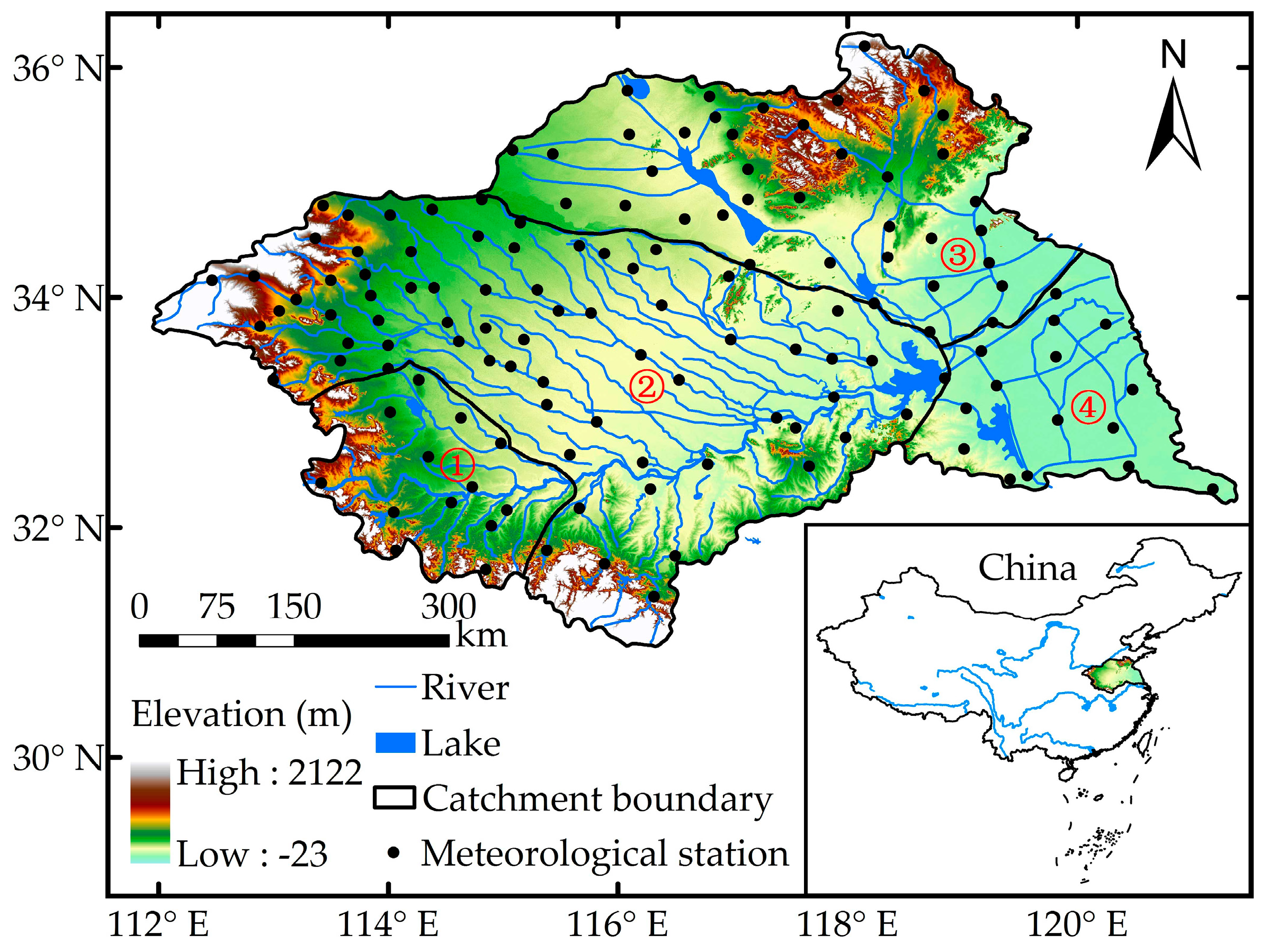
2.1. Study Area

The HRB is located between the Yangtze River and Yellow River Basin in Eastern China (111°55′ E–121°25′ E and 30°55′ N–36°36′ N) and has a watershed area of 270,000 km2. The length of the main stream is about 1000 km and the total river fall is about 200 m (Figure 1). Meanwhile, the HRB is situated in the climatic transition zone, which is recognized as the demarcation line (zero isotherm) between warm temperate and northern subtropical zones in China, accompanied with four distinctive seasons and moderate climate. The annual average precipitation is about 911 mm, with an uneven distribution pattern. More than 50% of the rainfall is concentrated during the monsoon season from June to September, accompanied by complex weather systems. Furthermore, the HRB is the most densely populated area and also a major grain-producing base in Eastern China [45], with the main crops—including wheat, rice, maize, potato, soybean, cotton, and canola—accounting for 17.3% of the total national grain yield.

2.2. Data Source

The datasets employed in the present study are mainly daily weather data obtained from 137 stations during 1961–2014 in the HRB, including the daily mean temperature (TA, °C), maximum temperature (Tmax, °C) and minimum temperature (Tmin, °C), relative humidity (RH, %), wind speed at 10 m (u10, m·s−1), and sunshine duration (SD, h). We obtained the weather data from the National Meteorological Information Center (NMIC) of the China Meteorological Administration (CMA) (http://data.cma.cn/site/index.html). The censored data are complemented through establishing linear interpolation between the neighboring weather stations. In this study, we defined five seasons as the growing season (April–October), spring (March–May), summer (June–August), autumn (September–November), and winter (December–February of the following year). The DEM (digital elevation model) datasets of 90 m spatial resolution (Figure 1) were acquired from the Internet (http://srtm.csi.cgiar.org/).

2.3. Reference Evapotranspiration Calculation

The FAO-56 Penman–Monteith (PM) model proposed by the Food and Agriculture Organization (FAO) has been regarded as an international recognized method to calculate ETref [2]. The FAO-56 PM model has a full theoretical basis which shows high accuracy [16]. The detailed formula is given as
E T r e f = 0.408 Δ ( R n G ) + γ 900 T + 273 u 2 ( e s e a ) Δ + γ ( 1 + 0.34 u 2 )
where E T r e f refers to the daily reference crop evapotranspiration (mm·day−1), Δ refers to the slope of vapor pressure curve (kPa·°C−1), R n refers to the net radiation at the crop height (MJ·m−2·day−1), G refers to the soil heat flux density (MJ·m−2·day−1), γ refers to the psychrometric constant (kPa·°C−1), T refers to the daily mean air temperature at 2 m (°C), u 2 refers to the wind speed at two-meter height (m·s−1), e s and e a refer to the saturation vapor pressure (kPa) and the actual vapor pressure (kPa), respectively.
For the convenience of E T r e f calculation, a conversion formula for wind speed was proposed by Allen et al. [2] as
u 2 = u z 4.87 ln ( 67.8 z 5.42 )
where u 2 refers to wind speed at two-meter height (m·s−1), u z refers to the wind speed at z meters above ground level.
Due to the lack of measured solar radiation ( R s ) data (MJ·m−2·day−1), R s is often calculated through sunshine hours, combed with the Angstrom formula [46]
R s = ( a s + b s n N ) R a
where R s refers to daily total solar radiation (MJ·m−2·day−1), R a refers to extraterrestrial radiation (MJ·m−2·day−1), n refers to daily sunshine hours (h), N refers to maximum possible sunshine hours (h), a s and b s are regression coefficients, according to Chen et al. [47], the values were set to 0.19 and 0.53, respectively [16].
Meanwhile, some sunshine duration data were missing in several inland stations of the HRB. In this regard, the radiation equation proposed by Hargreaves and Samani [48] was employed for calculating solar radiation ( R s ) through T m a x and T m i n as
R s = k R S × ( T m a x T m i n ) × R a
where k R S refers to the empirical coefficient and usually adopted the value of 0.16 for inland regions [48,49,50]. In order to verify the availability of the Hargreaves–Samani method, complete sunshine duration (SD) datasets of 39 meteorological stations located in the upper and middle HRB were employed in this study. The estimated SR and ETref calculated with Hargreaves–Samani (HS) method were compared with that calculated with SD during 1961–2014. The specific accuracy test can be found in Appendix A.
Finally, the net radiation ( R n ) is estimated by
R n = R n s R n l
R n s = ( 1 α ) R s
R n l = σ ( T m a x , K 4 + T m i n , K 4 2 ) ( 0.34 0.14 e a ) ( 1.35 R s R s 0 0.35 )
in which R n s refers to the incoming net shortwave radiation (MJ·m−2·day−1), α refers to the albedo of reference crop (value of 0.23), R n l refers to the net outgoing long-wave radiation (MJ·m−2·day−1), σ refers to the Stefan–Boltzmann constant (4.903 × 10⁻⁹ MJ·K−4·m−2·day−1), T m a x , K represents the maximum absolute temperature during 24 h (K = °C + 273.16), T m i n , K represents the minimum absolute temperature during 24 h (K = °C + 273.16), and R s o refers to clear-sky radiation. Furthermore, more specific approach procedures are provided in Allen et al.’s literature [2].

2.4. Trend Analysis

The worldwide recommended nonparametric test, Mann–Kendall (MK) test, was built to calculate the significance of a trend in hydro-meteorological time series [51,52]. The MK test is employed in this research to analyze temporal change trends of ETref and related meteorological variables [53,54,55]. It has an advantage which lies in its ability to test the linearity of a trend [31].
In order to identify slopes of ETref trends and climate factors, Theil–Sen’s estimator [55,56], a widely applied method to calculate the slope magnitude of the trend line, was adopted in this study
β = Median ( x j x i j i ) , 1 < i < j
where β refers to the estimated trend slope of the data series, x j and x i refer to the sequential data corresponding to time j and i , respectively.
Prior to applying the M–K test in this study, a pre-whitening method should be employed to eliminate the effect of a serial correlation on the trend value [57]. Yue et al. [58] improved this method and proposed an alternative approach, namely TFPW (trend-free pre-whitening), which is widely applied in many related study areas [17,30,59].

2.5. Spatial Interpolation Method

For investigating the spatial patterns of ETref and their trends, some spatial interpolation methods, such as spline, ordinary kriging (OK), and the inverse distance weighted (IDW), were implemented on account of datasets of meteorological stations being widely employed recently. Among these interpolation approaches, the IDW approach was adopted for the spatial pattern analysis in our study since it provides the lower mean error than the others [60,61]. The main justification for using the IDW technique is that it computes the spatially-interpolated values very quickly and accurately. All spatial distribution maps were prepared using the ArcGIS (version 9.3) software (Environmental Systems Research Institute (ESRI), Redlands, CA, USA).

2.6. Sensitivity Coefficient Estimation

For identifying sensitivities of ETref to meteorological factors, the differential method proposed by McCuen [27] is applied for this study
S ( v i ) = lim Δ v i / v i ( Δ E T r e f / E T r e f Δ v i / v i ) = E T r e f v i × v i E T r e f
where S ( v i ) refers to the sensitivity coefficient of E T r e f in relation to climatic variables ( v i ) . The positive (negative) sensitivities illustrate the E T r e f increases (decreases) are accompanied with the increases in v i . The absolute value of S ( v i ) represents the effect of a given v i on E T r e f . The specific derived calculation formula can be found from other literature [16].

2.7. Contributions of Climate Factors on ETref

The differential equation method indicates that the ETref is the function of meteorological variables. In previous studies [40,43], four meteorological variables (mean temperature (TA, °C), actual vapor pressure (ea, kPa), wind speed at two-meter height (WS, m·s−1), solar radiation (SR, MJ·m−2·day−1)) were selected as main influence factors to ETref, however, ea was not an independent variable, but a dependent variable function of TA and relative humidity (RH, %), considering the independence of each meteorological variable, we decided to replace the ea by RH in this study. Thus, the improved the differential equation method was used to estimate the individual contribution of each climate factor (TA, RH, WS, and SR) to ETref change trend based on the FAO-56 PM model. The detailed differential equation is
d E T r e f d t = E T r e f T A d T A d t + E T r e f R H d R H d t + E T r e f W S d W S d t + E T r e f S R d S R d t + ε
or, written briefly,
C _ E T r e f = C ( T A ) + C ( R H ) + C ( W S ) + C ( S R ) + ε
where C _ E T r e f refers to long term estimated trend of E T r e f , C ( T A ) , C ( R H ) , C ( W S ) , and C ( S R ) are contributions to E T r e f due to changes in T A , R H , W S , and S R , respectively. ε refers to the error term between the C _ E T r e f and E T r e f trends estimated by Theil–Sen’s estimator ( T _ E T r e f ). The contribution of each selected climate factor to the E T r e f trend can be obtained by calculating the averaged partial derivatives (Equations (9) and (10)) multiplied by the annual/seasonal tendency rates and the length of time (namely 365 or 366 for annual, 214 for growing season, 92 for spring and summer, 91 for autumn, and 90 or 91 for winter).

3. Results

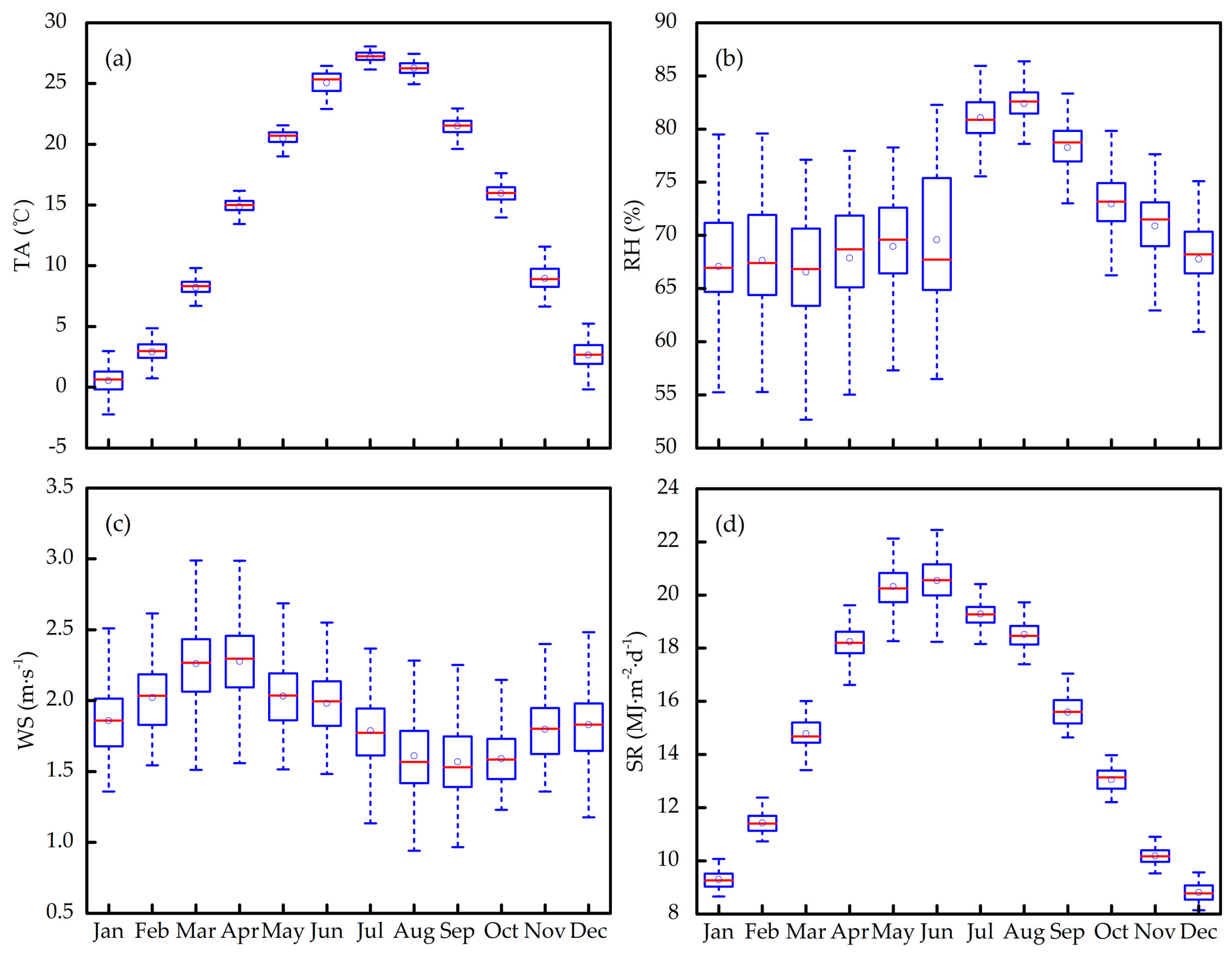
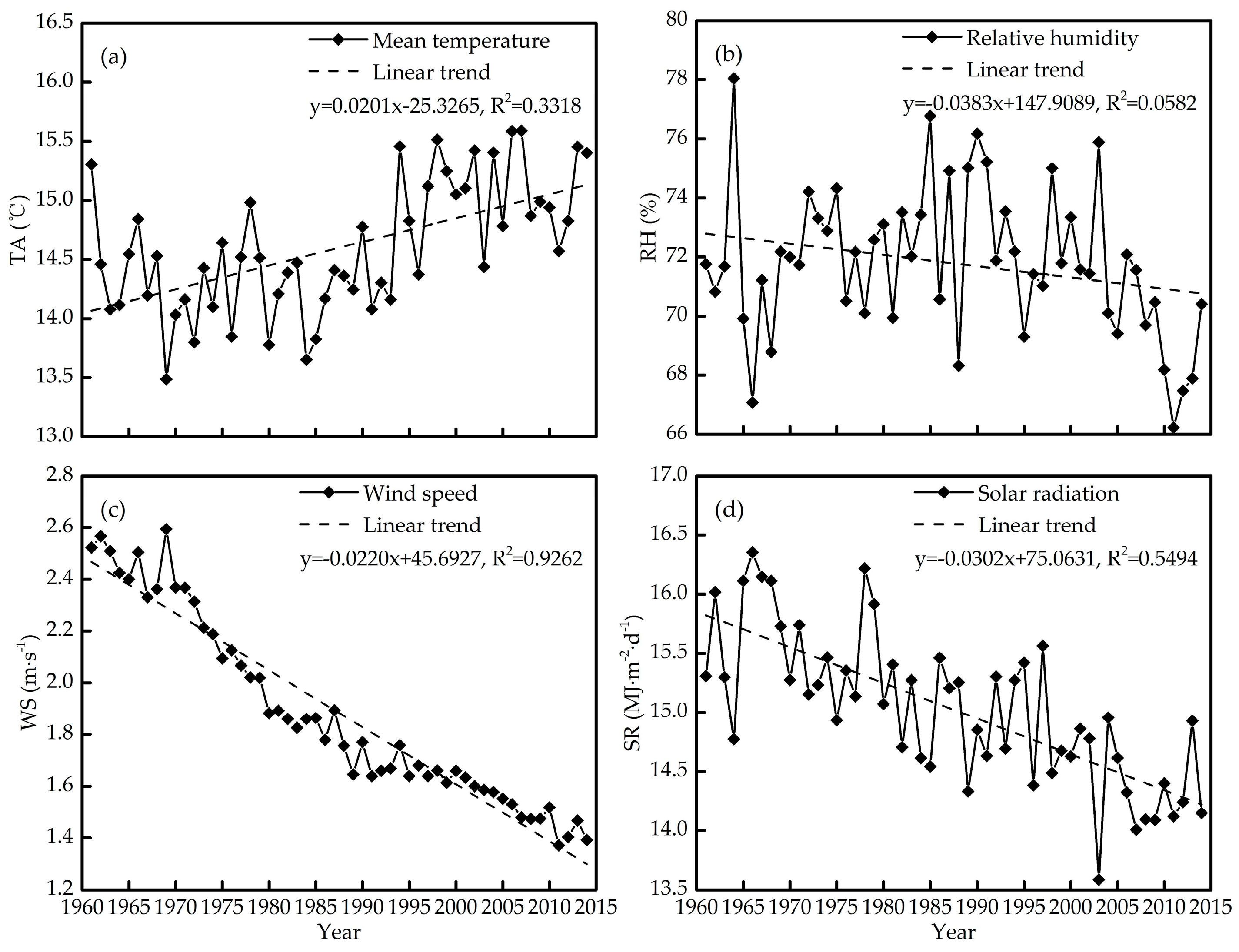
3.1. Variations of Climate Factors and Their Trend Analysis

Variations of monthly climate factors are shown in Figure 2. From Figure 2, monthly TA and SR exhibited similar variation patterns. The peak value occurred in June and July. The largest regional differences of SR were shown in spring and summer seasons, while the largest regional difference of TA exhibited in winter. Meanwhile, RH gradually increased before August and then decreased. Monthly WS values represent a fluctuating variation trend, the peak and valley values occurred in April and September, respectively.
The effects evaluation of climate factors to ETref was implemented by analyzing temporal trends of four meteorological parameters from 1961 to 2014 in the HRB. As from Figure 3, TA showed an overall upward trend in the past 54 years. It was noteworthy that a slow decreasing trend was observed before the 1990s and then a significantly increasing trend was observed. The RH fluctuated obviously, with a non-significant declining trend in the whole HRB. The WS and SR exhibited more significant declining trends in comparison with TA and RH.
The similar results can also be detected from Table 1. At the seasonal time scale, TA revealed a significant increasing trend in each season except the summer. Opposite to TA, RH exhibited a reverse change trend. Meanwhile, significant decreasing RH trends were found in the lower HRB in each season compared to the other regions. WS always exhibited a significant downward trend in all regions at each time scale, which could also be verified from Figure 3. The SR revealed a significant decreasing trend in the whole HRB in all time periods except spring.

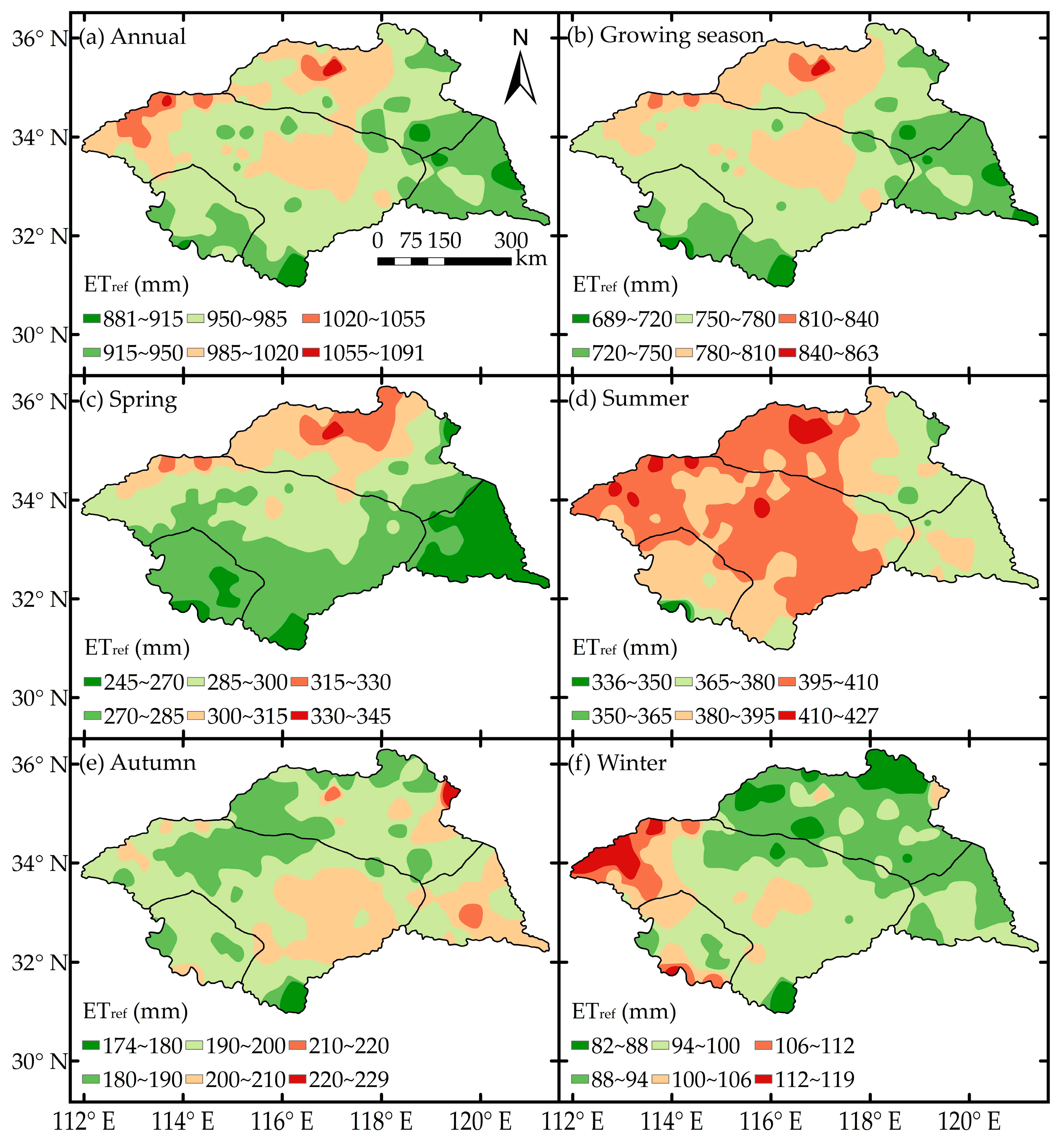
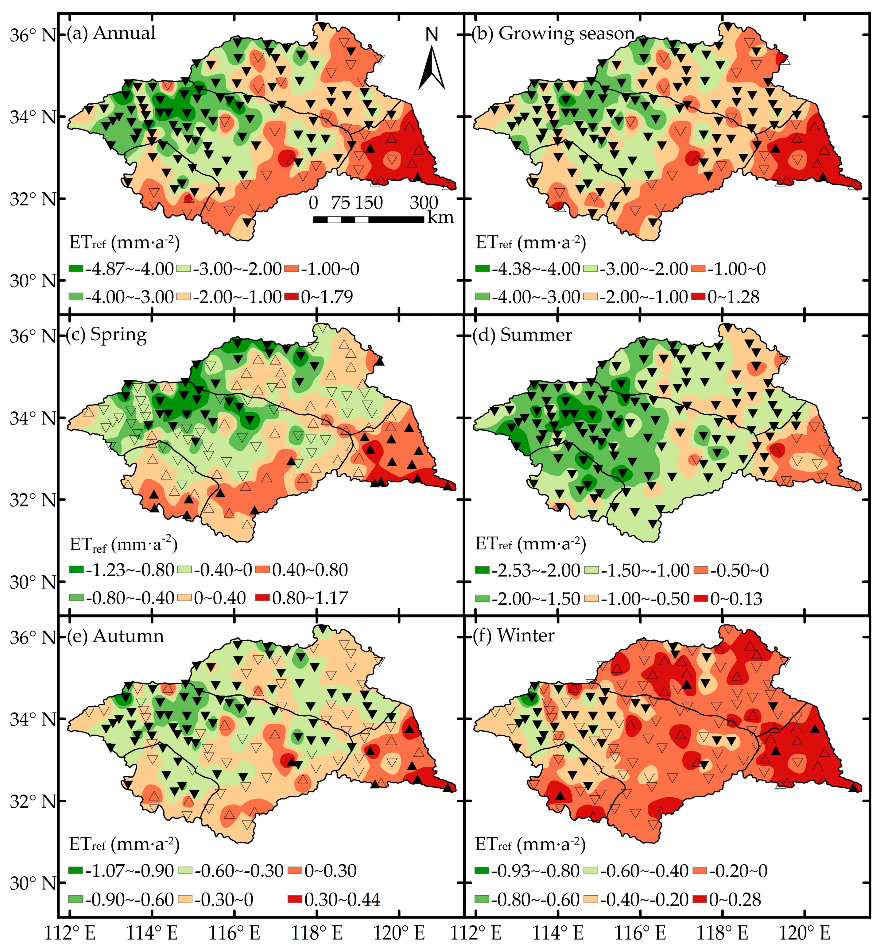
3.2. Variations of ETref and Their Trend Analysis

In order to obtain insights into the spatial distributions of annual and seasonal ETref in the HRB, the annual averaged ETref in each station from 1961 to 2014 was spatially interpolated using the IDW method (Figure 4). The annual ETref during the past 54 years in the HRB ranged from 881 mm to 1091 mm, with an average value of 969.56 mm. The higher values were observed in the north of the middle and Yi-Shu-Si River basins. Similar spatial distributions of ETref were identified during the growing season and spring, ranging from 689 mm to 863 mm, and from 245 mm to 345 mm, respectively. Meanwhile, the lower values of ETref mainly distributed in the upper and lower HRB. However, in the summer, the ETref was much higher than other seasons (336~427 mm), and the higher ETref values expanded to most parts of the upper and middle HRB also the Yi-Shu-Si River Basin. In autumn and winter, differences of ETref were smaller in the whole HRB. The higher values were observed in the southeast in autumn, and in the northwest in winter. In general, the ETref demonstrated a strong spatial heterogeneity in the whole HRB.
As shown in Table 2, at the annual time scale, a significant downward trend of ETref was found in the whole HRB (−1.894 mm·a−2), the upper and middle HRB and the Yi-Shu-Si River Basin. A non-significant upward trend was detected in the lower HRB (0.177 mm·a−2). The magnitude of the ETref trend followed the order: Middle > Upper > Yi-Shu-Si > Lower. During the growing season, the magnitude of the change rate was slightly lower than that at the annual time scale, while the spatial distribution was similar to that of the annual time scale. At the seasonal time scale, the magnitude of the change rates of ETref ranked in sequence as: summer > autumn > spring > winter in most of the HRB, except the lower HRB, while in the lower HRB the magnitude of change rates of ETref ranked in a sequence as: spring > summer > autumn > winter. In spring, only ETref in the lower HRB exhibited a significant increasing trend. In summer, ETref in all sub-regions showed significant decreasing trends. In autumn, ETref in the middle HRB and Yi-Shu-Si River Basin exhibited significant decreasing trends. However, in winter, no sub-region showed significant change trends. In the whole region, significant decreasing trends were observed at most time scales, except spring and winter, during which the change rate of ETref was the largest in the annual time scale.
The spatial distribution of seasonal ETref trends is displayed in Figure 5. Similar spatial distribution (increased from northwest to southeast) was observed at the annual time scale and during the growing season, ranging from −4.87 mm·a−2 to 1.79 mm·a−2 and −4.38 mm·a−2 to 1.28 mm·a−2, respectively. Among which, most decreasing trends were significant. In spring, the significant downward ETref trends were detected in the north parts of middle HRB and Yi-Shu-Si River Basin stations. However, ETref in the majority of stations of the lower HRB exhibited significant upward trends. Similar significant increasing trends could also be detected in some stations in the southern upper and middle HRB. In summer, more than 90% of stations demonstrated the significant decreasing trends of ETref, except the lower HRB. A general downward trend in ETref was observed in autumn and winter, with about 52% and 26% of stations exhibiting significant decreasing trends, respectively.

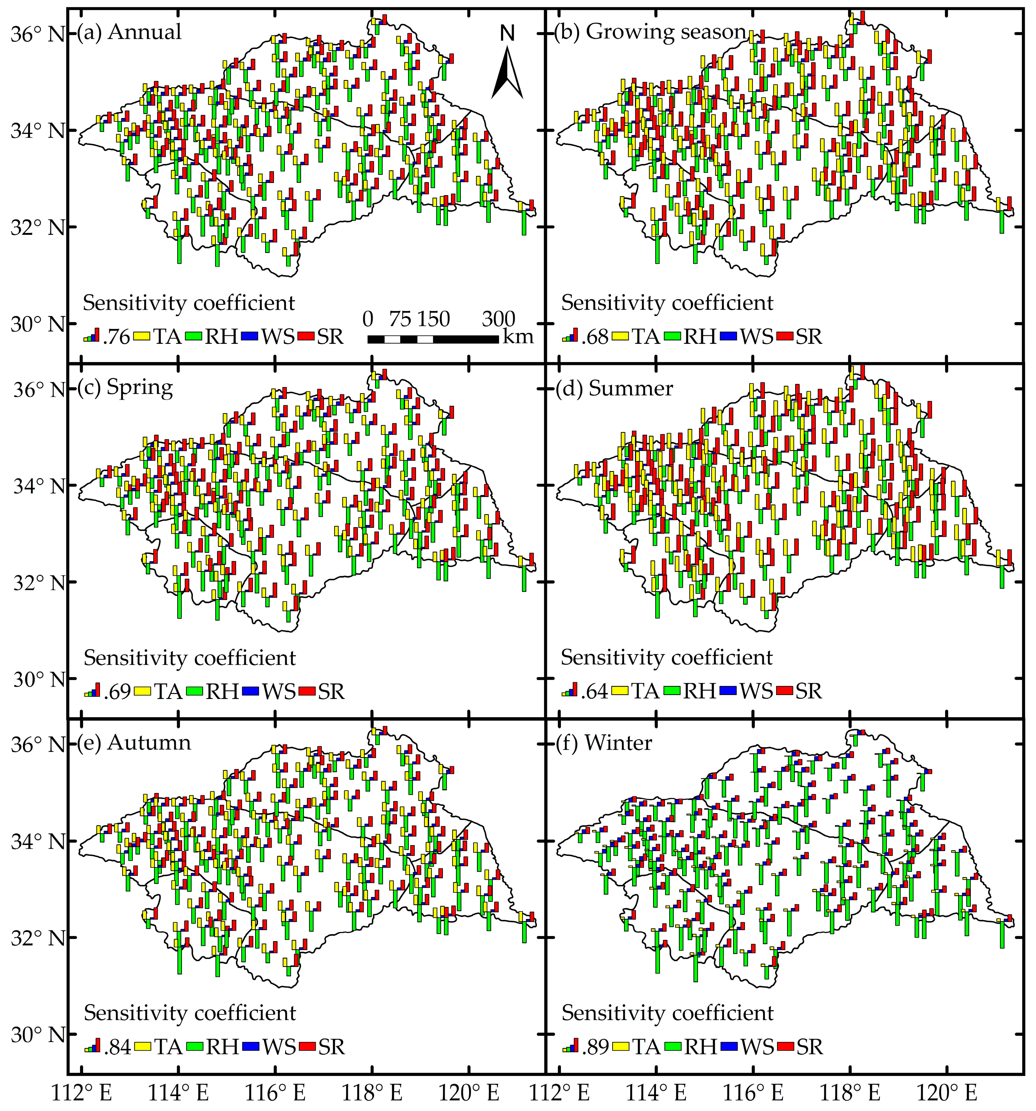
3.3. Sensitivity Coefficient of ETref to Climate Factors

To explore the effects of climate factors on ETref, sensitivity coefficients of air temperature, relative humidity, wind speed, and solar radiation in each time period of the HRB are shown in Table 3. Among all climate factors, only the RH showed negative sensitivity coefficients. Moreover, it declared that the ETref showed more sensitivity to RH, with SR, TA, and WS followed closely at the annual time scale in the whole HRB and every sub-region. In growing season, ETref in the upper and lower HRB showed the highest sensitivity to RH, while the whole HRB and other sub-regions showed the highest sensitivity to SR. At seasonal time scales, RH was the most sensitive factor in the whole HRB and all sub-regions except in summer. However, in summer, SR was the most sensitive factor in the whole HRB and most sub-regions, except the lower HRB. Meanwhile, RH was still the most sensitive factor in the lower HRB. In addition, the sensitivities of ETref to TA and SR were higher in the summer and during the growing season, but lower in the winter. The sensitivities of ETref to RH in autumn and winter seasons were much greater than that of other seasons. A detailed spatial distribution of sensitivity coefficients in each time period can be found in Figure 6.

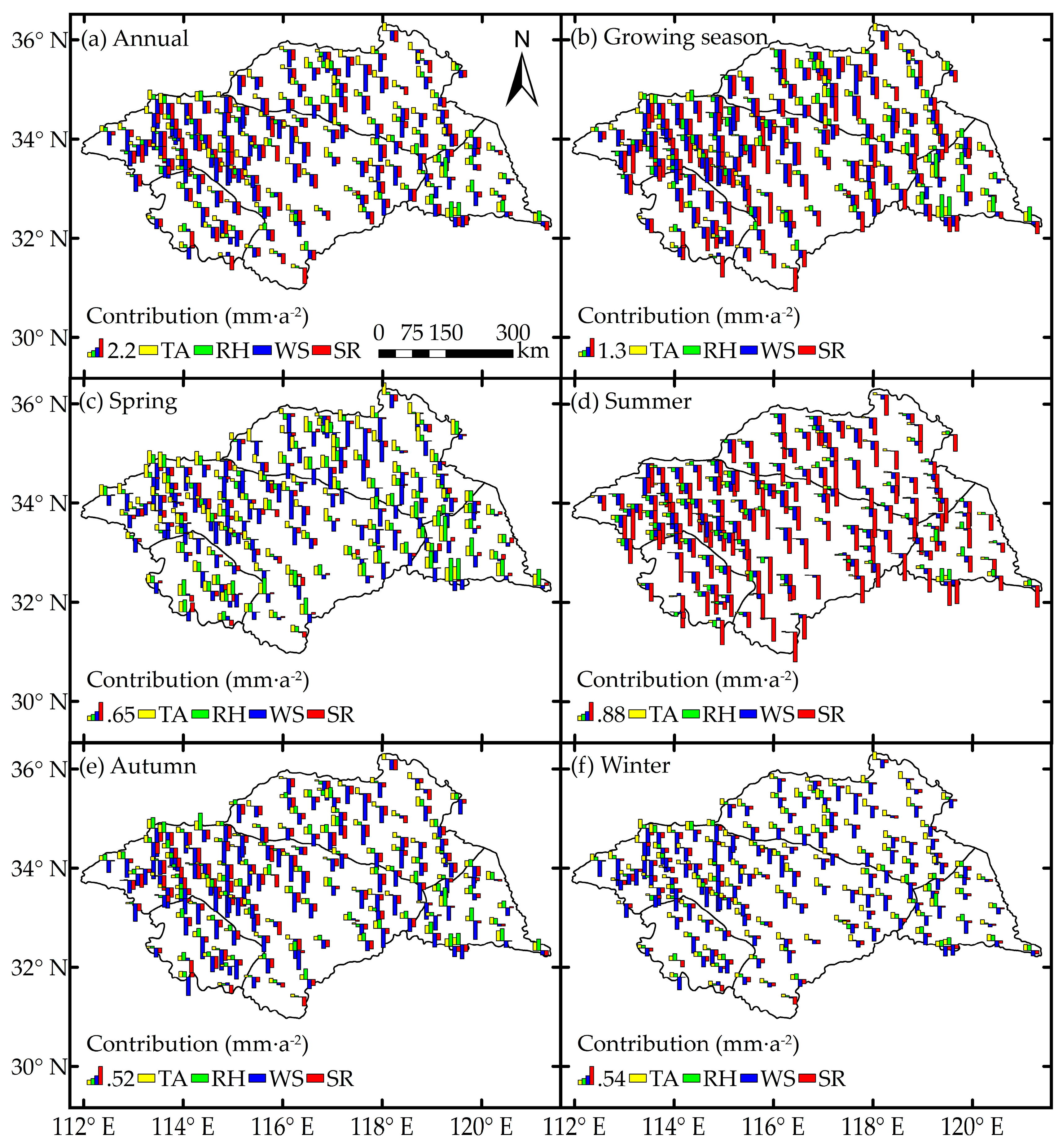
3.4. Quantitative Contributions of Climate Factors to ETref

The contributions from climate factors to the long-term ETref change trends were calculated by Equation (10). As observed from Figure 7, the change trends of the annual and seasonal ETref estimated using Equation (10) (C_ETref) were well fitted with ETref trends estimated by the Theil–Sen’s estimator (T_ETref). The R-squared value was larger than 0.94 in each time period and the slopes of the linear fit approximated to 1. The specific ETref change trends calculated from two approaches in all sub-regions in all time scales can be found in Table 4. The well-fitted relationship between C_ETref and T_ETref suggested that it was reasonable and reliable to adopt the four climate factors in Equation (10) to estimate its contributions to the change trends in ETref.
Based on the accuracy and applicability of the modified differential equation method, as shown from Table 4, TA and RH had positive contributions to ETref in the whole HRB and all sub-regions, except in some regions in summer. During the summer, TA showed small negative contributions in the upper and middle HRB, and RH showed small negative contributions in the whole HRB, upper, and middle HRB. WS and SR had negative contributions in the whole HRB and all sub-regions, except small positive contributions in the lower HRB in spring. This demonstrated that TA and RH were mainly responsible for the increasing trend in ETref, while WS and SR were mainly responsible for the decreasing trend in ETref. At an annual time scale, with spring, autumn and winter, WS contributed the most to ETref trends in the whole HRB and most sub-regions, except the lower HRB. In growing season and summer, SR contributed the most to ETref trends in the whole HRB and most sub-regions except the lower HRB. However, in the lower HRB, these factors contributed differently from other regions. The most contributive factor was RH at the annual time scale, growing season and in spring, then turned to SR in the summer and to WS in the autumn and winter. Further, it was noteworthy that positive contributions of TA and RH could not counteract the negative ones of WS and SR, which generated a significant downward trend (−1.894 mm·a−2) in the entire HRB at the annual time scale. Overall, this implies that the significant decrease of WS was the dominant contributing factor in ETref decline, followed by SR, TA, and RH, respectively. Similar findings were found in the upper, middle HRB and Yi-Shu-Si River Basin. Additionally, at seasonal time scales, the total contributions of the climatic variables in growing season and summer were much greater than that of the contributions in spring, autumn and winter seasons, which fit reasonably well with results from Table 1. Although the ETref was most sensitive to RH, the contribution of RH to ETref was generally less in the whole region. On the other hand, the ETref was the least sensitive to WS but the contribution of WS was the highest in the study area. Furthermore, the most vital contributing factor RH in the growing season and spring in the lower HRB merited more attention.
Figure 8 exhibits the seasonal and annual contributions of four climate factors to long-term ETref change trends in each meteorological station in the study period. WS was the dominate driving force to the changes in ETref at the annual time scale and spring, autumn, and winter seasons, which occupied 93, 94, 109, and 122 stations among a total of 137 stations in the whole HRB, respectively. On the contrary, in the same time scales, TA, RH, and SR were the dominate driving force to the changes in ETref, occupied 6, 6, 32 stations; 21, 21, 1 stations; 3, 8, 17 stations; and 10, 1, 4 stations among a total of 137 stations in the HRB, respectively. In the growing season and summer, SR contributed most to the change trends of ETref, especially in summer, which played a dominant role and occupied about 98.5% of stations of the entire HRB. Meanwhile, the TA, RH, WS, and SR acted as dominant parts in the changes of ETref at 1, 9, 45, and 82 stations during the growing season, respectively.

4. Discussion

4.1. Temporal Change Trends of ETref and Climate Factors in HRB

Global warming has become an accepted fact in the present era [31]. The warming rate in the global mean surface temperature from 1951 to 2012 was 0.012 °C·a−1. However, the significant increasing rate in TA (0.021 °C·a−1) in the entire HRB was two-fold larger than the global average [7], which was echoed by Sun et al. [62]. An interesting phenomenon was observed in this study that the TA in the upper and middle HRB demonstrated a slow and non-significant decreasing trend in summer.
Recently, the most significant decreasing rate of WS (−0.021 m·s−1·a−1) was detected in each time scale in the HRB. Similar results were also found elsewhere [63]. The decreasing WS rate agreed well with result of Guo et al. [64]. However, the magnitude of decreasing rate of WS in the HRB was much greater than those in the other river basins [1,21] and different areas in China [65,66], and also in East Asia [67]. The recent declining WS trend is mostly a result of large-scale atmospheric circulation patterns on account of climate warming [68], weakened Siberian High and East Asia Monsoon [69], descending temperature and pressure gradient [69,70,71], and intensified Asian zonal circulation patterns [72]. In addition, increased land surface roughness caused by the increased vegetation cover can give a reasonable explanation for the decreasing WS trend. Shan et al. [33] also found this was the reason for declining of WS rate, especially in Northwest China, where Chinese forestry and ecological projects have been implemented in large-scale forestation and reforestation. Furthermore, accelerated urbanization caused by population expansion and economic growth may be reasons for decreased WS, particularly in the regions near weather stations. Additionally, the decreasing WS will reduce the migration of water molecules, reducing the impact of aerodynamic force on ETref, therefore, lead to a downward trend in ETref [73]. However, the significant downward trend in the WS at each station of the HRB is still a debatable matter and needs further study.
Solar radiation (SR) as one crucial energy source, has found to be in a decreasing trend [1,21,43] which is similar to our results in the HRB. The radiation observation data showed that the SR decreased before 1980s [74,75], then gradually increased after 1990s, this phenomenon was named “from dimming to brightening” by Wild et al. [76]. As seen from Figure 3d, this phenomenon is not obvious in the HRB, and SR exhibited a significant downward trend at the rate of −0.03 MJ·m−2·day−1·a−1 in the annual time scale in the whole HRB. Possible reasons for this decreasing tendency are (1) the increased regional cloud cover [77]; (2) the increased aerosol loading due to the pollutants from anthropogenic emission [78,79]; (3) increased atmospheric moisture and the aggravated air-pollution caused by the energy depletion; and (4) the significant decreasing WS rate which restrained the spread of aerosols and pollutants [80].
In this study, we have drawn a conclusion that the TA increased significantly with a rate of 0.021 °C·a−1 in last 54 years in the HRB, whereas, the ETref exhibited a significant downward trend (−1.894 mm·a−2) in the whole region. The significant decreasing ETref in the HRB is in disagreement with climate warming result [81,82]. This differs from the earlier findings by Hulme et al. [83] and Goyal [82]. In fact, the two adverse change trends between the TA and ETref are titled the “evaporation paradox” proposed by Brutsaert and Parlange [13]. This paradoxical situation occurred in the HRB, especially in the upper and lower HRB and the Yi-Shu-Si River Basin. This finding is echoed with similar works in major basins of the Yangtze River [1], lower Yellow River [21], and Haihe River [84] in China and in many regions worldwide [5,11,85]. However, our results about the “evaporation paradox” slightly differ from the outcomes proposed by Thomas [15] which showed an increasing trend of ETref in the northeast and southwest region of China. This is because of the absence of a long-term meteorological dataset, a shortage of weather stations, and different study periods and areas in his research; whereas our study data source is a long-time series dataset (1961–2014) from 137 weather stations. McVicar et al. [63] conducted a worldwide research to study the ETref trend in the last three decades, then the downward tendency was detected in many parts worldwide. However, the lower HRB demonstrated an increasing ETref, this is also proved by results from Chu et al. [16].

4.2. Impact of Climate Factors to ETref Trends

The outcomes exhibited that the RH was the most sensitive factor of ETref in HRB, followed by SR, TA, and WS, respectively, which coincided with the conclusions proposed by Gong et al. [86] and Li et al. [31] in the Yangtze River Basin and also the Loess Plateau of Northern Shaanxi, China. However, in summer and during the growing season, the ETref showed the most sensitivity to SR, with TA, RH, and WS following, respectively. Similar findings could also be found in Spain [87] and the United States [88]. Additionally, the RH was the most sensitive factor in ETref in each time period of the lower HRB. All these discoveries are in accordance with the findings from Chu et al. [16] in Jiangsu Province, Eastern China. In fact, the meteorological factors influence ETref differently in different study areas. Huo et al. [14] indicated that the WS had the strongest sensitivity in arid Northwest China. Ye et al. [32] found SD was the dominating factor, with RH, WS, and TA following in the Poyang Lake catchment. Gao et al. [30] studied the sensitivities of ETref to the climate factors in the crop growth period in West Liao River Basin, then found SR was the most sensitive factor, with RH following. Moreover, Gao et al. [35] also have demonstrated SR was the most dominant factor for ETref in the same study area at the annual time scale, but varied at the seasonal time scale. The maximum temperature (Tmax) was the dominant climate factor for decreasing ETref in the Jing River Basin [8]. In other countries, Estévez et al. [87] proposed that ETref was most sensitive to TA, followed by RH, SR, and WS in Spain. Irmak et al. [88] found ETref was most sensitive to VPD (Vapor pressure deficit) in five locations of the United States, followed by WS in semiarid regions and SR in humid locations during the summer months. Thus, we concluded that diverse climatic conditions, different latitudes and elevations, and local environmental conditions are responsible for the various sensitivity analysis results of meteorological factors to ETref changes in various areas of the world.
In our research, we also found that WS was the dominant contributing climatic factor in the HRB. This result was echoed with results of Wang et al. [37], Zhang et al. [89], and McVicar et al. [63]. As shown above, RH was the most sensitive factor for ETref in the whole HRB, while WS was the least sensitive factor to the ETref in the same regions. This phenomenon may be due the change rate of WS was much greater than that of RH. Ultimately, WS exhibited a greater contribution to ETref trend. Thus, the higher contribution of RH in the lower HRB can be explained reasonably by the significant decreasing trend of RH in each time period shown in Table 1. However, the SR contributed more than WS in the growing season and summer, followed by TA and RH, respectively. This is mainly the result of the high values of SR concentrated in the growing season and summer (Figure 2), and its significantly decreasing trend during these periods (Table 1). Though the monthly change trend of TA was similar to SR, TA exhibited a significant increasing trend, except in summer and during the growing seasons, and these might be the main reason that SR exhibited a higher contribution to ETref than TA in the same period. However, the non-significance of the TA trend in summer and during the growing season was still unclear and needed to be further investigated. Similar to the sensitivities, the different meteorological factors contributions to ETref trends were discovered from different areas and in different climatic conditions. Fan et al. [29] reported that the ETref had different responses to climate factors across various climatic zones in China. Wang et al. [42] declared the decreasing net radiation was responsible for the ETref decrease in the three-river source area in China. The significantly increasing TA was the main reason for decreasing ETref in the entire Yellow River Basin [21]. Thus, effects of climate factors on ETref need to be further analyzed, especially in areas with varied climatic conditions, such as the HRB. Even though outcomes of this research indicated that the sensitivity and quantitative contribution analysis can delineate the importance of model parameters to output findings, which allows using it for making an accurate prediction, the methods of sensitivity and quantitative contribution analysis can be extended to other regions.

4.3. Uncertainties

We have taken into consideration four main climate factors from the FAO-56 PM model and analyze their effects on ETref trends. Although we have developed the differential equation method by using RH instead of ea in this study to reduce the estimation error, some errors may still exist due these four meteorological parameters influencing each other to some extent. Meanwhile, the systematic and random errors, inherent in meteorological measurements, could also affect the values of climate factors for estimating ETref [87]. At the same time, the influence of anthropogenic activities has acted as a primary part in recent years (e.g., Peterson et al. [81], Wang et al. [37]) and more uncertain factors are rising. Furthermore, attention should be drawn to some of the uncertainties that exist in the partial derivatives of the ETref, such as relative and fluctuating values during the long-term study period. The mean values of the partial derivatives of each climatic factor were used to calculate the contributions to ETref in our study which might generate more uncertainties [43]. In addition, on account of the lack of observed solar radiation data, the empirical parameters (as, bs) of the Angstrom equation listed in Equation (3) might have changed during the past 54 years’ time series due to the changed aerosol optical thickness in this area [90]. This is a crucial indication and may also constrain the measured effects of the changes in SR on ETref, ultimately leading to the underestimation of results by adopting this approximate value for calculating solar radiation from sunshine duration [16].

5. Conclusions

We found the variation of ETref could not generate obvious spatial diversity, with the higher values concentrated in the north of middle HRB and Yi-Shu-Si River Basin. ETref showed a significant downward trend (p < 0.001) in the upper and middle HRB, and also the Yi-Shu-Si River Basin, particularly in summer and during the growing season, while ETref exhibited a slight increasing trend in the lower HRB, especially significantly in spring. All these phenomena could be explained reasonably by the variations in climate factors. TA had a significant upward trend in most time scales except in summer; RH fluctuated obviously and showed a significant decreasing trend in the lower HRB in each time scale; WS exhibited a significant decreasing trend in all sub-regions in each time scale; and SR had a significant downward trend in most time scales, except in spring. According to the sensitivities of ETref to climate factors in the HRB, the negative RH showed as the most sensitive factor in most sub-regions, with the positive SR, TA, and WS following, respectively. However, the ETref was most sensitive to SR in the growing season and summer in most sub-regions except the lower HRB. Based on the developed differential equation method, WS was the most contributing factor, followed by SR, TA, and RH in most time scales, while the SR contributed most to the ETref trends in growing season and summer in most sub-regions, except the lower HRB. Generally, the negative contribution values of the WS and SR would offset the positive ones of TA and RH, which lead to an overall significant decreasing trend in ETref in relevant sub-regions and time scales. However, in the lower HRB, the RH contributed most to ETref, with WS, TA, and SR following, which could be responsible for the slightly increasing trend in ETref here.
This research deepens insights into the change patterns of regional climate and ETref, which will offer a scientific theoretical foundation for future investigation on the actual evapotranspiration (ET) of this basin. This research also plays a pivotal role in analogical agricultural crop production and irrigation management. The estimation of ET by using the physical model, as well as remote sensing and land use data, in recent years is an important study, which will delineate the spatiotemporal patterns of ET and its controlling factors in the HRB in the context of rapid urbanization and climatic change. It deserves further investigation and can be a promising extension of this present research work.

Acknowledgments

The fund of this research comes from the Postgraduate Research & Practice Innovation Program of Jiangsu Province (KYCX17_0885) and China Special Fund for Meteorological Research in the Public Interest (GYHY201106043; GYHY201506001). We also thank the editors and two anonymous reviewers for their constructive comments and suggestions that helped us to improve the quality of this manuscript.

Author Contributions

Meng Li and Ronghao Chu analyzed the data and wrote the paper. Shuanghe Shen supervised the whole research. Abu Reza Md. Towfiqul Islam modified and polished the English in this paper.

Conflicts of Interest

The authors declare no conflict of interest.

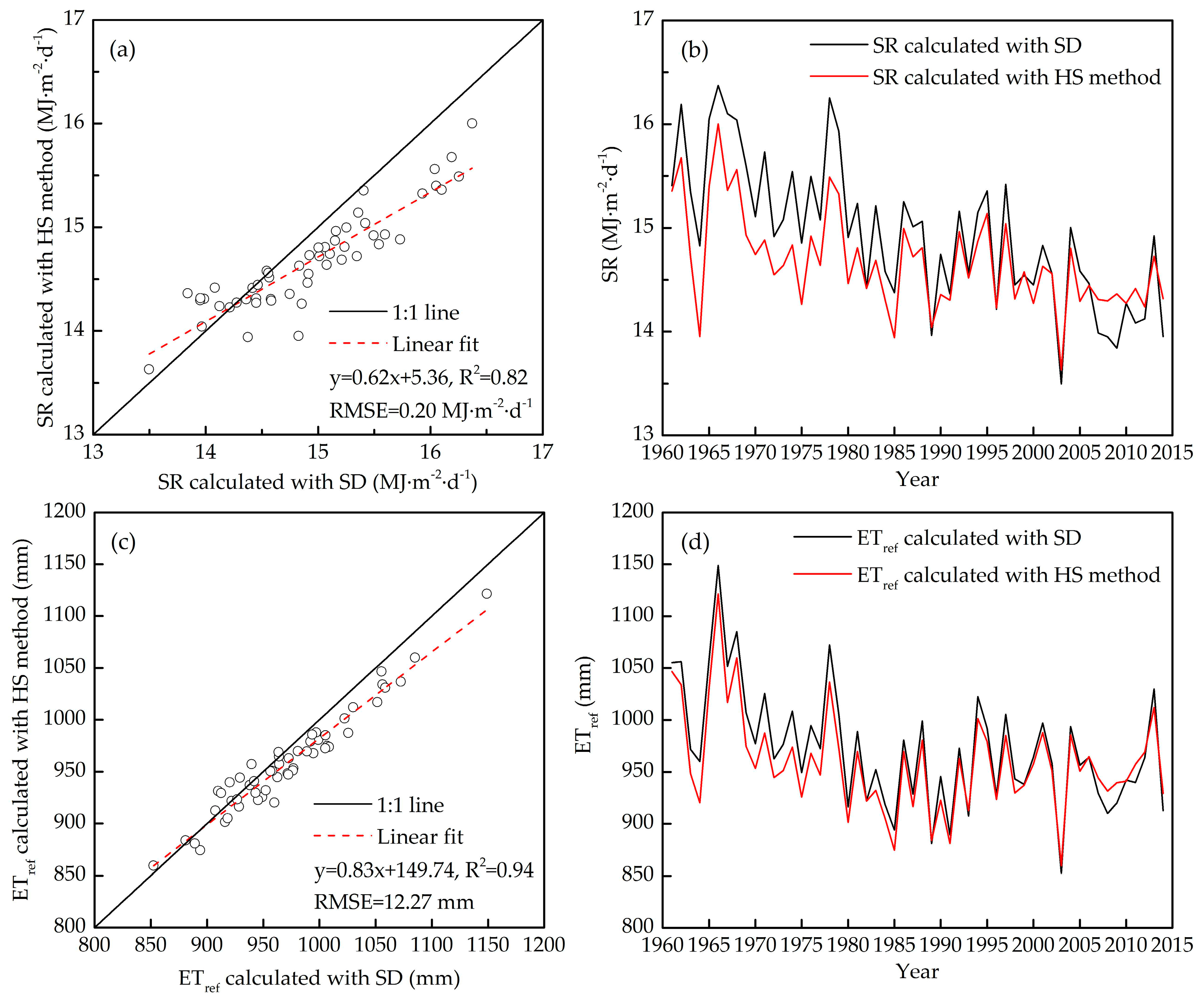
Appendix A. Validation of the Hargreaves–Samani Method for Estimating Solar Radiation

Figure A1. (a) The fitting precision of the SR_HS (SR calculated with Hargreaves–Samani method), (b) compared with the SR_SD (SR calculated with SD), and (c) the fitting precision of ETref_HS (ETref calculated with Hargreaves–Samani method) compared with (d) the ETref_SD (ETref calculated with SD).
Water 10 00144 g0a1

References

  1. Xu, C.Y.; Gong, L.; Jiang, T.; Chen, D.; Singh, V.P. Analysis of spatial distribution and temporal trend of reference evapotranspiration and pan evaporation in Changjiang (Yangtze River) catchment. J. Hydrol. 2006, 327, 81–93. [Google Scholar] [CrossRef]
  2. Allen, R.G.; Pereira, L.S.; Raes, D.; Smith, M. Crop Evapotranspiration—Guidelines for Computing Crop Water Requirements—FAO Irrigation and Drainage Paper 56; FAO: Rome, Italy, 1998. [Google Scholar]
  3. Zhao, L.; Xia, J.; Sobkowiak, L.; Li, Z. Climatic Characteristics of Reference Evapotranspiration in the Hai River Basin and Their Attribution. Water 2014, 6, 1482–1499. [Google Scholar] [CrossRef]
  4. Thomas, A. Development and properties of 0.25-degree gridded evapotranspiration data fields of China for hydrological studies. J. Hydrol. 2008, 358, 145–158. [Google Scholar] [CrossRef]
  5. Jhajharia, D.; Shrivastava, S.K.; Sarkar, D.; Sarkar, S. Temporal characteristics of pan evaporation trends under the humid conditions of northeast India. Agric. For. Meteorol. 2009, 149, 763–770. [Google Scholar] [CrossRef]
  6. Zuo, H.; Chen, B.; Wang, S.; Guo, Y.; Zuo, B.; Wu, L.; Gao, X. Observational study on complementary relationship between pan evaporation and actual evapotranspiration and its variation with pan type. Agric. For. Meteorol. 2016, 222, 1–9. [Google Scholar] [CrossRef]
  7. Alexander, L.V.; Allen, S.K.; Bindoff, N.L.; Bréon, F.-M.; Church, J.A.; Cubasch, U.; Emori, S.; Forster, P.; Friedlingstein, P.; Gillett, N.; et al. Climate change 2013: The physical science basis, in contribution of Working Group I (WGI) to the Fifth Assessment Report (AR5) of the Intergovernmental Panel on Climate Change (IPCC). Science 2013, 129, 83–103. [Google Scholar]
  8. Xu, L.; Shi, Z.; Wang, Y.; Zhang, S.; Chu, X.; Yu, P.; Xiong, W.; Zuo, H.; Wang, Y. Spatiotemporal variation and driving forces of reference evapotranspiration in Jing River Basin, northwest China. Hydrol. Process. 2015, 29, 4846–4862. [Google Scholar] [CrossRef]
  9. McMahon, T.A.; Finlayson, B.L.; Peel, M.C. Historical developments of models for estimating evaporation using standard meteorological data. WIREs Water 2016, 3, 788–818. [Google Scholar] [CrossRef]
  10. Cong, Z.T.; Yang, D.W.; Ni, G.H. Does evaporation paradox exist in China? Hydrol. Earth Syst. Sci. 2009, 13, 357–366. [Google Scholar] [CrossRef]
  11. Limjirakan, S.; Limsakul, A. Trends in Thailand pan evaporation from 1970 to 2007. Atmos. Res. 2012, 108, 122–127. [Google Scholar] [CrossRef]
  12. Breña-Naranjo, J.A.; Laverde-Barajas, M.Á.; Pedrozo-Acuña, A. Changes in pan evaporation in Mexico from 1961 to 2010. Int. J. Climatol. 2016, 23, 361–387. [Google Scholar] [CrossRef]
  13. Brutsaert, W.; Parlange, M.B. Hydrologic cycle explains the evaporation paradox. Nature 1998, 396, 30. [Google Scholar] [CrossRef]
  14. Huo, Z.; Dai, X.; Feng, S.; Kang, S.; Huang, G. Effect of climate change on reference evapotranspiration and aridity index in arid region of China. J. Hydrol. 2013, 492, 24–34. [Google Scholar] [CrossRef]
  15. Thomas, A. Spatial and temporal characteristics of potential evapotranspiration trends over China. Int. J. Climatol. 2000, 20, 381–396. [Google Scholar] [CrossRef]
  16. Chu, R.; Li, M.; Shen, S.; Islam, A.R.M.T.; Cao, W.; Tao, S.; Gao, P. Changes in reference evapotranspiration and its contributing factors in Jiangsu, a major economic and agricultural province of eastern China. Water 2017, 9, 486. [Google Scholar] [CrossRef]
  17. Dinpashoh, Y.; Jhajharia, D.; Fard, A.F.; Singh, V.P.; Kahya, E. Trends in reference crop evapotranspiration over Iran. J. Hydrol. 2011, 399, 422–433. [Google Scholar] [CrossRef]
  18. Tabari, H.; Aghajanloo, M.B. Temporal pattern of aridity index in Iran with considering precipitation and evapotranspiration trends. Int. J. Climatol. 2013, 33, 396–409. [Google Scholar] [CrossRef]
  19. Chaouche, K.; Neppel, L.; Dieulin, C.; Pujol, N.; Ladouche, B.; Martin, E.; Salas, D.; Caballero, Y. Analyses of precipitation, temperature and evapotranspiration in a French Mediterranean region in the context of climate change. Comptes Rendus Geosci. 2010, 342, 234–243. [Google Scholar] [CrossRef]
  20. Palumbo, A.D.; Vitale, D.; Campi, P.; Mastrorilli, M. Time trend in reference evapotranspiration: Analysis of a long series of agrometeorological measurements in Southern Italy. Irrig. Drain. Syst. 2011, 25, 395–411. [Google Scholar] [CrossRef]
  21. Liu, Q.; Yang, Z.; Cui, B.; Sun, T. The temporal trends of reference evapotranspiration and its sensitivity to key meteorological variables in the Yellow River Basin, China. Hydrol. Process. 2010, 24, 2171–2181. [Google Scholar] [CrossRef]
  22. Zuo, D.; Xu, Z.; Yang, H.; Liu, X. Spatiotemporal variations and abrupt changes of potential evapotranspiration and its sensitivity to key meteorological variables in the Wei River basin, China. Hydrol. Process. 2012, 26, 1149–1160. [Google Scholar] [CrossRef]
  23. Vörösmarty, C.J.; Sahagian, D. Anthropogenic disturbance of the terrestrial water cycle. Bioscience 2000, 50, 753–765. [Google Scholar] [CrossRef]
  24. Rezaei, M.; Valipour, M.; Valipour, M. Modelling evapotranspiration to increase the accuracy of the estimations based on the climatic parameters. Water Conserv. Sci. Eng. 2016, 1, 197–207. [Google Scholar] [CrossRef]
  25. Valipour, M.; Sefidkouhi, M.A.G.; Sarjaz, M.R. Selecting the best model to estimate potential evapotranspiration with respect to climate change and magnitudes of extreme events. Agric. Water Manag. 2017, 180, 50–60. [Google Scholar] [CrossRef]
  26. Tegos, A.; Malamos, N.; Efstratiadis, A.; Tsoukalas, I.; Karanasios, A.; Koutsoyiannis, D. Parametric Modelling of Potential Evapotranspiration: A Global Survey. Water 2017, 9, 795. [Google Scholar] [CrossRef]
  27. McCuen, R.H. A sensitivity and error analysis of procedures used for estimating evaporation. J. Am. Water Resour. Assoc. 1974, 10, 486–497. [Google Scholar] [CrossRef]
  28. Yin, Y.; Wu, S.; Chen, G.; Dai, E. Attribution analyses of potential evapotranspiration changes in China since the 1960s. Theor. Appl. Climatol. 2010, 101, 19–28. [Google Scholar] [CrossRef]
  29. Fan, J.; Wu, L.; Zhang, F.; Xiang, Y.; Zheng, J. Climate change effects on reference crop evapotranspiration across different climatic zones of China during 1956–2015. J. Hydrol. 2016, 542, 923–937. [Google Scholar] [CrossRef]
  30. Gao, Z.; He, J.; Dong, K.; Bian, X.; Li, X. Sensitivity study of reference crop evapotranspiration during growing season in the West Liao River basin, China. Theor. Appl. Climatol. 2016, 124, 1–17. [Google Scholar] [CrossRef]
  31. Li, C.; Wu, P.T.; Li, X.L.; Zhou, T.W.; Sun, S.K.; Wang, Y.B.; Luan, X.B.; Yu, X. Spatial and temporal evolution of climatic factors and its impacts on potential evapotranspiration in Loess Plateau of Northern Shaanxi, China. Sci. Total Environ. 2017, 589, 165–172. [Google Scholar] [CrossRef] [PubMed]
  32. Ye, X.; Li, X.; Liu, J.; Xu, C.; Zhang, Q. Variation of reference evapotranspiration and its contributing climatic factors in the Poyang Lake catchment, China. Hydrol. Process. 2015, 28, 6151–6162. [Google Scholar] [CrossRef]
  33. Shan, N.; Shi, Z.; Yang, X.; Gao, J.; Cai, D. Spatiotemporal trends of reference evapotranspiration and its driving factors in the Beijing-Tianjin Sand Source Control Project Region, China. Agric. For. Meteorol. 2015, 200, 322–333. [Google Scholar] [CrossRef]
  34. Wang, Z.; Xie, P.; Lai, C.; Chen, X.; Wu, X.; Zeng, Z.; Li, J. Spatiotemporal variability of reference evapotranspiration and contributing climatic factors in China during 1961–2013. J. Hydrol. 2017, 544, 97–108. [Google Scholar] [CrossRef]
  35. Gao, Z.; He, J.; Dong, K.; Li, X. Trends in reference evapotranspiration and their causative factors in the West Liao River basin, China. Agric. For. Meteorol. 2017, 232, 106–177. [Google Scholar] [CrossRef]
  36. Li, Z.; Li, Z.; Xu, Z.; Zhou, X. Temporal variations of reference evapotranspiration in Heihe River basin of China. Hydrol. Res. 2013, 44, 904–916. [Google Scholar] [CrossRef]
  37. Wang, W.; Shao, Q.; Peng, S.; Xing, W.; Yang, T.; Luo, Y.; Yong, B.; Xu, J. Reference evapotranspiration change and the causes across the Yellow River Basin during 1957–2008 and their spatial and seasonal differences. Water Resour. Res. 2012, 48, 1–27. [Google Scholar] [CrossRef]
  38. Nouri, M.; Homaee, M.; Bannayan, M. Quantitative trend, sensitivity and contribution analyses of reference evapotranspiration in some arid environments under climate change. Water Resour. Manag. 2017, 31, 2207–2224. [Google Scholar] [CrossRef]
  39. Roderick, M.L.; Rotstayn, L.D.; Farquhar, G.D.; Hobbins, M.T. On the attribution of changing pan evaporation. Geophys. Res. Lett. 2007, 34, 251–270. [Google Scholar] [CrossRef]
  40. Zheng, H.; Liu, X.; Liu, C.; Dai, X.; Zhu, R. Assessing contributions to panevaporation trends in Haihe River Basin, China. J. Geophys. Res. 2009, 114, 144–153. [Google Scholar] [CrossRef]
  41. Liu, Q.; Mcvicar, T.R. Assessing climate change induced modification of Penman potential evaporation and runoff sensitivity in a large water-limited basin. J. Hydrol. 2012, 464–465, 352–362. [Google Scholar] [CrossRef]
  42. Wang, Q.; Wang, J.; Zhao, Y.; Li, H.; Zhai, J.; Yu, Z.; Zhang, S. Reference evapotranspiration trends from 1980 to 2012 and their attribution to meteorological drivers in the three-river source region, China. Int. J. Climatol. 2016, 36, 3759–3769. [Google Scholar] [CrossRef]
  43. Liu, X.; Zhang, D. Trend analysis of reference evapotranspiration in Northwest China: The roles of changing wind speed and surface air temperature. Hydrol. Process. 2013, 27, 3941–3948. [Google Scholar] [CrossRef]
  44. Ye, J.; He, Y.; Pappenberger, F.; Cloke, H.L.; Manful, D.; Li, Z. Evaluation of ECMWF medium-range ensemble forecasts of precipitation for river basins. Q. J. R. Meteorol. Soc. 2013, 140, 1615–1628. [Google Scholar] [CrossRef] [Green Version]
  45. Yan, J.; Yu, J.; Tao, G.; Vos, J.; Bouman, B.A.M.; Xie, G.H.; Meinke, H. Yield formation and tillering dynamics of direct-seeded rice in flooded and nonflooded soils in the Huai River Basin of China. Field Crop. Res. 2010, 116, 252–259. [Google Scholar] [CrossRef]
  46. Angstrom, A. Solar and terrestrial radiation. Report to the international commission for solar research on actinometric investigations of solar and atmospheric radiation. Q. J. R. Meteorol. Soc. 1924, 50, 121–126. [Google Scholar] [CrossRef]
  47. Chen, R.; Kang, E.; Yang, J.; Lu, S.; Zhao, W. Validation of five global radiation models with measured daily data in China. Energy Convers. Manag. 2004, 45, 1759–1769. [Google Scholar] [CrossRef]
  48. Hargreaves, G.H.; Samani, Z.A. Estimating potential evapotranspiration. J. Irrig. Drain. Div. 1982, 108, 225–230. [Google Scholar]
  49. Hargreaves, G.H.; Allen, R.G. History and evaluation of Hargreaves evapotranspiration equation. J. Irrig. Drain. Eng. 2003, 129, 53–63. [Google Scholar] [CrossRef]
  50. Allen, R.G. Self-Calibrating Method for Estimating Solar Radiation from Air Temperature. J. Hydrol. Eng. 1997, 2, 56–67. [Google Scholar] [CrossRef]
  51. Tabari, H.; Somee, B.S.; Zadeh, M.R. Testing for long-term trends in climatic variables in Iran. Atmos. Res. 2011, 100, 132–140. [Google Scholar] [CrossRef]
  52. Zhang, Q.; Liu, C.; Xu, C.; Xu, Y.; Jiang, T. Observed trends of annual maximum water level and streamflow during past 130 years in the Yangtze River basin, China. J. Hydrol. 2006, 324, 255–265. [Google Scholar] [CrossRef]
  53. Mann, H.B. Nonparametric test against trend. Econometrica 1945, 13, 245–259. [Google Scholar] [CrossRef]
  54. Kendall, M.G. Rank Correlation Methods; Griffin: London, UK, 1975. [Google Scholar]
  55. Theil, H. A Rank Invariant Method of Linear and Polynomial Regression Analysis; Nederlandse Akademie Van Wetenschappen: Amsterdam, The Netherlands, 1950. [Google Scholar]
  56. Sen, P.K. Estimates of the Regression Coefficient Based on Kendall’s Tau. J. Am. Stat. Assoc. 1968, 63, 1379–1389. [Google Scholar] [CrossRef]
  57. Von Storch, H.; Navarra, A. Analysis of Climate Variability: Applications of Statistical Techniques, Misuses of Statistical Analysis in Climate Research; Springer: Berlin, Germany, 1995. [Google Scholar]
  58. Yue, S.; Pilon, P.; Phinney, B.; Cavadias, G. The influence of autocorrelation on the ability to detect trend in hydrological series. Hydrol. Process. 2002, 16, 1807–1829. [Google Scholar] [CrossRef]
  59. Kumar, S.; Merwade, V.; Kam, J.; Thurner, K. Streamflow trends in Indiana: Effects of long term persistence, precipitation and subsurface drains. J. Hydrol. 2009, 374, 171–183. [Google Scholar] [CrossRef]
  60. Tegos, A.; Malamos, N.; Koutsoyiannis, D. A parsimonious regional parametric evapotranspiration model based on a simplification of the Penman-Monteith formula. J. Hydrol. 2015, 524, 708–717. [Google Scholar] [CrossRef]
  61. Zhao, C.; Nan, Z.; Cheng, G. Methods for modelling of temporal and spatial distribution of air temperature at landscape scale in the southern Qilian mountains, China. Ecol. Model. 2005, 189, 209–220. [Google Scholar]
  62. Sun, F.; Yang, X.; Lu, S.; Yang, S. The contrast analysis on the average and extremum temperature trend in Northeast China. Sci. Meteorol. Sin. 2006, 26, 157–163. [Google Scholar]
  63. McVicar, T.R.; Roderick, M.L.; Donohue, R.J.; Li, L.T.; Niel, T.G.V.; Thomas, A.; Grieser, J.; Jhajharia, D.; Himri, Y.; Mahowald, N.M.; et al. Global review and synthesis of trends in observed terrestrial near-surface wind speeds: Implications for evaporation. J. Hydrol. 2012, 416–417, 182–205. [Google Scholar] [CrossRef]
  64. Guo, H.; Xu, M.; Hu, Q. Changes in near-surface wind speed in China: 1969–2005. Int. J. Climatol. 2015, 31, 349–358. [Google Scholar] [CrossRef]
  65. Mcvicar, T.R.; Roderick, M.L. Atmospheric science: Winds of change. Nat. Geosci. 2010, 3, 747–748. [Google Scholar] [CrossRef]
  66. Song, Z.W.; Zhang, H.L.; Snyder, R.L.; Anderson, F.E.; Chen, F. Distribution and trends in reference evapotranspiration in the North China Plain. J. Irrig. Drain. Eng. 2010, 136, 240–247. [Google Scholar] [CrossRef]
  67. Vautard, R.; Cattiaux, J.; Yiou, P.; Thépaut, J.-N.; Ciais, P. Northern Hemisphere atmospheric stilling partly attributed to an increase in surface roughness. Nat. Geosci. 2010, 3, 756–761. [Google Scholar] [CrossRef]
  68. Shi, Z.; Xu, L.; Yang, X.; Guo, H.; Dong, L.; Song, A.; Zhang, X.; Shan, N. Trends in reference evapotranspiration and its attribution over the past 50 years in the Loess Plateau, China: Implications for ecological projects and agricultural production. Stoch. Environ. Res. Risk Assess. 2017, 31, 257–273. [Google Scholar] [CrossRef]
  69. Xu, M.; Chang, C.-P.; Fu, C.; Qi, Y.; Robock, A.; Robinson, D.; Zhang, H.-M. Steady decline of East Asian monsoon winds, 1969–2000: Evidence from direct ground measurements of wind speed. J. Geophys. Res. 2006, 111, 906–910. [Google Scholar] [CrossRef]
  70. You, Q.; Kang, S.; Flügel, W.-A.; Pepin, N.; Yan, Y.; Huang, J. Decreasing wind speed and weakening latitudinal surface pressure gradients in the Tibetan Plateau. Clim. Res. 2010, 42, 57–64. [Google Scholar] [CrossRef]
  71. Lin, C.; Yang, K.; Qin, J. Observed surface and upper-air wind speed changes over China since 1960. J. Clim. 2012, 26, 2891–2903. [Google Scholar] [CrossRef]
  72. Kwon, M.H.; Jhun, J.G.; Ha, K.J. Decadal change in East Asian summer monsoon circulation in the mid-1990s. Geophys. Res. Lett. 2007, 34, 377–390. [Google Scholar] [CrossRef]
  73. Teh, C.B.S. Introduction to Mathematical Modeling of Crop Growth: How the Equations Are Derived and Assembled into a Computer Program; BrownWalker Press: Boca Raton, FL, USA, 2006. [Google Scholar]
  74. Stanhill, G.; Cohen, S. Global dimming: A review of the evidence for a widespread and significant reduction in global radiation with discussion of its probable causes and possible agricultural consequences. Agric. For. Meteorol. 2001, 107, 255–278. [Google Scholar] [CrossRef]
  75. Liepert, B.G. Observed reductions of surface solar radiation at sites in the United States and worldwide from 1961 to 1990. Geophys. Res. Lett. 2002, 29, 1–4. [Google Scholar] [CrossRef]
  76. Wild, M.; Gilgen, H.; Roesch, A.; Ohmura, A.; Long, C.N.; Dutton, E.G.; Forgan, B.; Kallis, A.; Russak, V.; Tsvetkov, A. From dimming to brightening: Decadal changes in solar radiation at Earth’s surface. Science 2005, 308, 847–850. [Google Scholar] [CrossRef] [PubMed]
  77. Stjern, C.W.; Ansson, J.E.K.; Hansen, A.W. Global dimming and global brightening-an analysis of surface radiation and cloud cover data in northern Europe. Int. J. Climatol. 2008, 29, 643–653. [Google Scholar] [CrossRef]
  78. Qian, Y.; Wang, W.; Leung, L.R.; Kaiser, D.P. Variability of solar radiation under cloud-free skies in China: The role of aerosols. Geophys. Res. Lett. 2007, 34, 1–5. [Google Scholar] [CrossRef]
  79. Che, H.Z.; Shi, G.Y.; Zhang, X.Y.; Arimoto, R.; Zhao, J.Q.; Xu, L.; Wang, B.; Chen, Z.H. Analysis of 40 years of solar radiation data from China, 1961–2000. Geophys. Res. Lett. 2005, 32, 1–5. [Google Scholar] [CrossRef]
  80. Yang, Y.H.; Zhao, N.; Hu, Y.K.; Zhou, X.Y. Effect of wind speed on sunshine hours in three cities in northern China. Clim. Res. 2009, 39, 149–157. [Google Scholar] [CrossRef]
  81. Peterson, T.C.; Golubev, V.S.; Groisman, P.Y. Evaporation losing its strength. Nature 1995, 377, 687–688. [Google Scholar] [CrossRef]
  82. Goyal, R.K. Sensitivity of evapotranspiration to global warming: A case study of arid zone of Rajasthan (India). Agric. Water Manag. 2004, 69, 1–11. [Google Scholar] [CrossRef]
  83. Hulme, M.; Zhao, Z.; Jiang, T. Recent and future climate change in East Asia. Int. J. Climatol. 1994, 14, 637–658. [Google Scholar] [CrossRef]
  84. Tang, B.; Tong, L.; Kang, S.; Zhang, L. Impacts of climate variability on reference evapotranspiration over 58 years in the Haihe river basin of north China. Agric. Water Manag. 2011, 97, 1506–1516. [Google Scholar] [CrossRef]
  85. Roderick, M.L.; Farquhar, G.D. Changes in Australian pan evaporation from 1970 to 2002. Int. J. Climatol. 2004, 24, 1077–1090. [Google Scholar] [CrossRef]
  86. Gong, L.; Xu, C.-Y.; Chen, D.; Halldin, S.; Chen, Y.D. Sensitivity of the Penman-Monteith reference evapotranspiration to key climatic variables in the Changjiang (Yangtze River) basin. J. Hydrol. 2006, 329, 620–629. [Google Scholar] [CrossRef]
  87. Estévez, J.; Gavilán, P.; Berengena, J. Sensitivity analysis of a Penman–Monteith ttype equation to estimate reference evapotranspiration in Southern Spain. Hydrol. Process. 2009, 23, 3342–3353. [Google Scholar] [CrossRef]
  88. Irmak, S.; Payero, J.; Martin, D.; Irmak, A.; Howell, T. Sensitivity analyses and sensitivity coefficients of standardized daily ASCE-Penman-Monteith equation. J. Irrig. Drain. Eng. 2006, 132, 564–578. [Google Scholar] [CrossRef]
  89. Zhang, Y.; Liu, C.; Tan, Y.; Yang, Y. Trends in pan evaporation and reference and actual evapotranspiration across the Tibetan Plateau. J. Geophys. Res. 2007, 112, 1–12. [Google Scholar] [CrossRef]
  90. Li, M.; Chu, R.; Shen, S.; Islam, A.R.M.T. Dynamic analysis of pan evaporation variations in the Huai River Basin, a climate transition zone in eastern China. Sci. Total Environ. 2018, 625, 496–509. [Google Scholar] [CrossRef] [PubMed]
Figure 1. The location of the Huai River Basin (HRB) in China and its spatial distributions of the elevation, meteorological stations and the river system, four sub-regions represent ①: Upper HRB, ②: Middle HRB; ③: Yi-Shu-Si River Basin; and ④: Lower HRB, respectively.
Water 10 00144 g001
Figure 2. Box plots show the monthly variations of (a) TA; (b) RH; (c) WS; and (d) SR in the HRB.
Water 10 00144 g002
Figure 3. Temporal trends of (a) TA; (b) RH; (c) WS; and (d) SR in the HRB during 1961–2014.
Water 10 00144 g003
Figure 4. Spatial distribution maps of (a) annual; (b) growing season; (c) spring; (d) summer; (e) autumn; and (f) winter ETref during 1961–2014 in the HRB.
Water 10 00144 g004
Figure 5. Spatial distribution maps of (a) annual; (b) growing season; (c) spring; (d) summer; (e) autumn; and (f) winter ETref trends during 1961–2014 in the HRB. The upward and downward triangles represent increasing and decreasing ETref trends The solid black triangle represents a significance level of 0.05.
Water 10 00144 g005
Figure 6. Spatial distribution maps of (a) annual; (b) growing season; (c) spring; (d) summer; (e) autumn; and (f) winter sensitivity coefficients during 1961–2014 in the HRB.
Water 10 00144 g006
Figure 7. Relationship between the calculated C_ETref and the estimated ETref trend (T_ETref) by Theil–Sen’s estimator.
Water 10 00144 g007
Figure 8. Spatial distribution patterns of contributions of climate factors to ETref in (a) annual; (b) growing season; (c) spring; (d) summer; (e) autumn; and (f) winter during 1961–2014 in the HRB.
Water 10 00144 g008
Table 1. Seasonal and annual trend analyses of climatic factors in each region of the HRB during 1961–2014.
RegionClimatic FactorAnnualGrowing SeasonSpringSummerAutumnWinter
ZβZβZβZβZβZβ
UpperTA (°C)3.480.01 ***2.180.010 *3.760.034 ***−0.91−0.0072.510.015 *2.760.025 **
RH (%)−1.55−0.035−0.79−0.027−2.81−0.133 **2.090.056 *−1.79−0.065−0.85−0.051
WS (m·s−1)−9.37−0.019 ***−9.13−0.019 ***−8.30−0.020 ***−8.16−0.019 ***−8.31−0.020 ***−8.18−0.020 ***
SR (MJ·m−2·day−1)−5.09−0.030 ***−4.36−0.038 ***−0.39−0.005−5.13−0.062 ***−2.27−0.018 *−3.52−0.023 ***
MiddleTA (°C)3.570.018 ***2.040.010 *3.570.030 ***−0.60−0.0043.180.016 **3.490.032 ***
RH (%)−0.55−0.015−0.13−0.005−1.33−0.0641.390.040−1.61−0.061−0.64−0.039
WS (m·s−1)−9.71−0.022 ***−9.58−0.021 ***−9.04−0.024 ***−9.09−0.020 ***−8.94−0.021 ***−8.56−0.023 ***
SR (MJ·m−2·day−1)−6.01−0.035 ***−5.42−0.045 ***−1.09−0.012−5.82−0.072 ***−3.10−0.026 ***−4.15−0.029 ***
Yi-Shu-SiTA (°C)4.860.025 ***3.630.017 ***4.460.035 ***1.030.0063.670.021 ***4.430.040 ***
RH (%)−1.79−0.042−1.60−0.035−1.66−0.075−0.57−0.012−1.31−0.050−1.01−0.053
WS (m·s−1)−8.97−0.021 ***−8.85−0.021 ***−8.55−0.025 ***−8.46−0.019 ***−7.80−0.019 ***−7.58−0.020 ***
SR (MJ·m−2·day−1)−5.82−0.030 ***−5.18−0.038 ***−1.34−0.010−5.82−0.062 ***−3.27−0.025 **−3.83−0.023 ***
LowerTA (°C)4.670.027 ***3.880.023 ***4.790.039 ***1.310.0124.070.026 ***3.890.034 ***
RH (%)−4.79−0.109 ***−4.74−0.120 ***−4.01−0.178 ***−3.36−0.085 ***−3.60−0.107 ***−2.95−0.098 **
WS (m·s−1)−8.76−0.021 ***−8.27−0.019 ***−8.58−0.025 ***−7.46−0.017 ***−7.33−0.019 ***−7.88−0.022 ***
SR (MJ·m−2·day−1)−4.10−0.018 ***−3.27−0.023 **0.950.009−4.18−0.056 ***−1.45−0.009−2.42−0.017 *
WholeTA (°C)4.060.021 ***2.780.013 **3.880.032 ***0.100.0013.520.018 ***3.770.035 ***
RH (%)−1.64−0.038−1.28−0.028−1.76−0.0830.180.005−1.87−0.062−0.97−0.054
WS (m·s−1)−9.64−0.021 ***−9.50−0.020 ***−8.98−0.024 ***−9.00−0.019 ***−8.64−0.020 ***−8.40−0.022 ***
SR (MJ·m−2·day−1)−5.73−0.030 ***−5.25−0.040 ***−0.72−0.007−5.79−0.066 ***−3.07−0.022 **−3.80−0.025 ***
Note: *, **, and *** denote the significance levels of 0.05, 0.01, and 0.001, respectively. β is the estimated slope trend of ETref, β > 0 and β < 0 signify an upward and a downward trend, respectively. Z is the Mann–Kendall test statistic.
Table 2. Seasonal and annual trends of ETref (mm·a−2) during 1961–2014 in each region of the HRB.
RegionAnnualGrowing SeasonSpringSummerAutumnWinter
ZβZβZβZβZβZβ
Upper−3.49−1.787 ***−3.55−1.578 ***0.690.197−4.97−1.567 ***−1.76−0.253−1.12−0.138
Middle−4.74−2.561 ***−4.92−2.287 ***−1.06−0.331−5.43−1.596 ***−2.73−0.400 **−1.82−0.235
Yi-Shu-Si−3.88−1.556 ***−3.83−1.446 ***−0.60−0.153−4.43−1.094 ***−2.25−0.276 *−0.39−0.044
Lower0.450.1770.150.0623.040.660 **−1.97−0.498 *0.910.1000.930.075
Whole−4.09−1.894 ***−4.25−1.772 ***−0.39−0.122−4.64−1.307 ***−2.40−0.308 *−1.24−0.143
Note: *, **, and *** denote the significance levels of 0.05, 0.01, and 0.001, respectively. β refers to the estimated slope trend of ETref, β > 0 and β < 0 signify an upward and a downward trend, respectively. Z is the Mann–Kendall test statistic.
Table 3. Annual and seasonal sensitivity coefficients of ETref to the main climate factors in each region of the HRB during 1961–2014.
RegionSensitivity CoefficientAnnualGrowing SeasonSpringSummerAutumnWinter
UpperS(TA)0.4630.6340.4930.6950.5410.122
S(RH)−0.963−0.764−0.853−0.675−1.032−1.301
S(WS)0.1150.0770.0890.0550.1310.184
S(SR)0.6420.7370.6660.7930.6300.480
MiddleS(TA)0.4610.6400.4980.7000.5440.102
S(RH)−0.850−0.669−0.739−0.597−0.907−1.165
S(WS)0.1400.0950.1140.0730.1520.222
S(SR)0.6150.7200.6370.7790.6090.436
Yi-Shu-SiS(TA)0.4360.6390.4800.6990.5360.028
S(RH)−0.813−0.663−0.678−0.642−0.852−1.082
S(WS)0.1560.1000.1380.0650.1690.253
S(SR)0.5820.7010.5910.7780.5770.383
LowerS(TA)0.4810.6620.4880.7240.5880.122
S(RH)−1.128−0.929−1.037−0.864−1.135−1.478
S(WS)0.1110.0670.0740.0420.1380.191
S(SR)0.6140.7180.6360.7830.6020.433
WholeS(TA)0.4590.6430.4930.7030.5490.091
S(RH)−0.892−0.713−0.777−0.653−0.939−1.204
S(WS)0.1380.0900.1120.0650.1520.222
S(SR)0.6100.7170.6290.7810.6020.427
Note: The bold fonts represent the most sensitive factors in each time period.
Table 4. Annual and seasonal contributions (mm·a−2) of the main climate factors to ETref in each region of the HRB during 1961–2014.
RegionContributionAnnualGrowing SeasonSpringSummerAutumnWinter
UpperC(TA)0.5720.2480.324−0.0560.1030.133
C(RH)0.2360.1110.296−0.1530.1210.066
C(WS)−1.300−0.775−0.334−0.281−0.386−0.289
C(SR)−1.217−1.203−0.057−1.028−0.191−0.122
C_ETref−1.710−1.6190.228−1.517−0.353−0.211
T_ETref−1.787−1.5780.197−1.567−0.253−0.138
MiddleC(TA)0.5840.2250.297−0.0390.1210.158
C(RH)0.0540.0080.141−0.1230.1050.047
C(WS)−1.777−1.038−0.488−0.405−0.446−0.389
C(SR)−1.383−1.358−0.115−1.123−0.257−0.125
C_ETref−2.523−2.163−0.166−1.690−0.476−0.309
T_ETref−2.561−2.287−0.331−1.596−0.400−0.235
Yi-Shu-SiC(TA)0.8310.4170.3750.0650.1590.200
C(RH)0.2890.1530.1770.0200.0920.078
C(WS)−1.622−0.977−0.567−0.321−0.395−0.325
C(SR)−1.133−1.130−0.096−0.986−0.224−0.087
C_ETref−1.635−1.537−0.112−1.223−0.368−0.134
T_ETref−1.556−1.446−0.153−1.094−0.276−0.044
LowerC(TA)0.8780.5230.3790.1190.1890.168
C(RH)1.0120.7680.4670.2420.2430.154
C(WS)−0.983−0.540−0.285−0.157−0.285−0.241
C(SR)−0.753−0.7200.056−0.869−0.109−0.069
C_ETref0.1550.0310.617−0.6650.0390.012
T_ETref0.1770.0620.660−0.4980.1000.075
WholeC(TA)0.6790.3100.3290.0040.1370.167
C(RH)0.2540.1510.207−0.0460.1220.071
C(WS)−1.608−0.944−0.473−0.345−0.411−0.347
C(SR)−1.222−1.204−0.080−1.047−0.223−0.108
C_ETref−1.897−1.687−0.018−1.434−0.374−0.217
T_ETref−1.894−1.772−0.122−1.307−0.308−0.143
Note: The bold fonts represent the most contributing factor in each time period.

