A Note on One- and Three-Dimensional Infiltration Analysis from a Mini Disc Infiltrometer

Abstract

Disc infiltrometers are used to characterize soil hydraulic properties. The purpose of this study was to determine the difference between three- and one-dimensional infiltration and to calculate the infiltration shape parameter γ from a proposed analytical infiltration equation. One- and three-dimensional infiltration tests were done on three repacked soils (loam, sandy loam, and silty clay loam) for two negative pressure heads. A mini disc infiltrometer of a radius of 22.5 mm with suction that ranged from −5 mm to −70 mm was used. The difference between experimental three- and one-dimensional cumulative infiltration was linear with time, which confirmed the proposed equation. In this study, the shape parameter γ seems not to be seriously affected by the soil type and acquires values from 0.561 to 0.615, i.e., smaller than the value γ = 0.75, which is widely used. With these values, the criteria proposed for calculating hydraulic conductivity using three-dimensional infiltration data may be fulfilled in most soils.

1. Introduction

For better agricultural water management, it is necessary to understand the infiltration process, which is a fundamental process through which cultivated crops absorb water and nutrients in a perpetual cycle to satisfy atmospheric energy and water demands. Knowledge of both soil water infiltration characteristics, saturated hydraulic conductivity and soil sorptivity, of the upper soil layers is essential for the modeling of the field infiltration process for agricultural water management and hydrological applications. Disc infiltrometers, among other experimental apparatuses used in situ for determining these two infiltration characteristics, have been extensively used in recent decades [1,2,3,4,5]. Disc infiltrometers allow measurements of infiltration with a constant and small negative pressure head, h₀, at the soil surface and have been extensively used to measure the near-saturated hydraulic conductivity, K₀, and sorptivity, S₀ [1,2,3,4,5]. Among the different types of disc infiltrometers, mini disc infiltrometers have the advantage of being portable and using small volumes of water, making them suitable for spatial variability studies [6,7,8].

If a disc infiltrometer is placed on the soil surface and the water flow below it is not artificially restricted, then a three-dimensional flow with axial symmetry could be established. Smettem et al. [1] showed that three-dimensional infiltration is related with one-dimensional infiltration with an extra added term which is linear with time and suggested the following approximate analytical expression:

$${\mathrm{I}}_{3\mathrm{D}}={\mathrm{I}}_{1\mathrm{D}}+\frac{{\mathsf{\gamma }\mathrm{S}}_0^2}{\mathrm{r}\left({\mathsf{\theta }}_0-{\mathsf{\theta }}_{\mathrm{n}}\right)}\mathrm{t},$$

(1)

where the subscript 3D and 1D refer to the three- and one-dimensional infiltration process, subscript 0 refers to values on the supply boundary where the pressure head is h₀ (L), subscript n refers to the initial conditions, r is the disc radius (L), S₀ is sorptivity (L T^−0.5), and γ is a shape parameter.

The shape parameter γ was originally set equal to $\sqrt{0.3}$ by Smettem et al. [1], but as it was shown, a better agreement between experimental and analytical solutions data could be established when γ = 0.75. The above findings were obtained from experiments in a sandy loam soil with a circular disc infiltrometer of 37.5 mm radius and with a quarter disc infiltrometer of 150 mm radius. Later, the shape parameter γ was revised to be 0.6 < γ < 0.8 by Haverkamp et al. [4]. They used the experimental data of Quadri et al. (1994) [9] performed in a sandy soil with a disc infiltrometer of radius r = 60 mm and a constant pressure head h₀ = −50 mm imposed on the soil surface. Smettem et al. (1995) [10] used a double-disc infiltrometer in such a way that they were able to collect infiltration measured data simultaneously, both from three- and one-dimensional infiltration and, more importantly, under the same initial and boundary conditions. From these experimental data and applying Equation (1), they found that the value of γ was 0.726. Lassabatere et al. (2009) [11] studied the cumulative infiltration from a disc of 10 cm radius for four soils (sand, loam, silt, and silty clay) at different initial water content. From the comparison of semianalytical equations of infiltration with the infiltration data, they found that the quasiexact formulation gives better results for γ values between 0.75 and 1. Moreover, from the results, it was shown that the value of γ depends on the soil type. More specifically, for the loam and the silt soils, the optimized values of γ were close to the value of 0.75, but for the sand and the silty clay soil, they were much bigger (1.03 and 0.977, respectively). In addition, Warrick and Lazarovitch (2007) [12] reported lower values for γ for medium textured soils and larger values for coarser soils and finer soils. Additionally, Lassabatere et al. (2009) [11] estimated the value of γ for four studied soils, based on the equation of Fuentes et al. (1992) [13], where significantly lower values γ from the values 0.75 till 1.03 were obtained. The values of γ from the equation of Fuentes et al. (1992) [13] were between 0.575 and 0.593. Warick et al. (2007) [14] and Warrick and Lazarovitch (2007) [12] reported, also, that the value of γ depends on the geometry of the infiltration source.

In order to calculate the value of γ from Equation (1), based on experimental data of the difference I_3D−I_1D, an accurate estimation of the parameters S₀ and Δθ is required. Various methodologies have been proposed to determine K₀ and S₀ from three-dimensional infiltration data from a circular source at soil surface using a disc infiltrometer. Among these, some are based on steady-state flow data and others on transient flow data [2,4,15,16,17,18,19,20]. In the case of a steady-state flow from a circular source with constant negative pressure head at soil surface, the analytical solution of Wooding [21] is used. Wooding’s equation is applied by assuming that the soil is homogenous and isotropic, and the initial water content is uniform. Due to uncertainties about the time at which a steady-state infiltration regime is attained, together with the fact that useful information is lost by ignoring the transient stage, several researchers use a transient three-dimensional infiltration equation for disc infiltrometers [22]. However, several expressions for transient infiltration [3,4,18] have in common the following two-term cumulative infiltration equation analogous to Philip [23]:

$$\mathrm{I}={\mathrm{C}}_1\sqrt{\mathrm{t}}+{\mathrm{C}}_2\mathrm{t}$$

(2)

where I is the cumulative infiltration (L) and the coefficients C₁ (L T^−0.5) and C₂ (L T⁻¹) differ among the expressions used [22]. Haverkamp et al. [4] established a physically based model for a disc infiltrometer for short and medium times:

$${\mathrm{I}}_{3\mathrm{D}}={\mathrm{S}}_0\sqrt{\mathrm{t}}+\frac{2-\mathsf{\beta }}{3}{\mathrm{K}}_0\mathrm{t}+\frac{{\mathsf{\gamma }\mathrm{S}}_0^2}{\mathrm{r}\left({\mathsf{\theta }}_0-{\mathsf{\theta }}_{\mathrm{n}}\right)}\mathrm{t}$$

(3)

where the subscript 3D refers to the three-dimensional infiltration process, subscript 0 refers to values on the supply boundary where the pressure head is h₀ (L), subscript n refers to the initial conditions, r is the disc radius (L), and β is a shape factor lying between 0 and 1, with common value 0.6. The first term on the right-hand side in Equation (3) represents vertical capillary flow and dominates infiltration during the initial stage. The second term represents gravity-driven vertical flow and the third term represents lateral capillary flow.

Haverkamp et al. [4] related C₁ and C₂ to S₀ and Κ₀ through the expressions as follows:

C₁ = S₀

(4)

$${\mathrm{C}}_2=\frac{2-\mathsf{\beta }}{3}{\mathrm{K}}_0+\frac{{\mathsf{\gamma }\mathrm{S}}_0^2}{\mathrm{r}\left({\mathsf{\theta }}_0-{\mathsf{\theta }}_{\mathrm{n}}\right)}$$

(5)

From Equations (4) and (5), it appears that the value of the C₁ parameter is independent of the infiltrometer radius r, while the value of C₂ is dependent on it.

Vandervaere et al. [19] established the following criterion for the reliability of the K₀ estimation from Equation (5), where γ = 0.75:

$$\frac{{\mathsf{\gamma }\mathrm{C}}_1^2}{\mathrm{r}\left({\mathsf{\theta }}_0-{\mathsf{\theta }}_{\mathrm{n}}\right)}<\frac{{\mathrm{C}}_2}{2}$$

(6)

That is, when the second right term of Equation (5) is large (dominant term in C₂), then the calculation of K₀ is impossible.

Dohnal et al. [24], by performing a numerical analysis on infiltration data from a mini disc infiltrometer of 12 soils, found that the second term of Equation (5) resulted in high values and therefore, K₀ could not be calculated by the Haverkamp et al. [4] model in all cases studied. Thus, they assumed the above criterion is too restrictive and suggested that it could be replaced by another, softer one:

$$\frac{{\mathsf{\gamma }\mathrm{C}}_1^2}{\mathrm{r}\left({\mathsf{\theta }}_0-{\mathsf{\theta }}_{\mathrm{n}}\right)}<{\mathrm{C}}_2$$

(7)

Various linear fitting techniques of Equation (2) (e.g., [5,25]) have been proposed for the calculation of the C₁ and C₂ parameters, which allow the possibility to detect the possible inadequacy of Equation (2), as well as the scattering of data points. Smiles and Knight [25] proposed the linearizing of Equation (2) by dividing both sides by $\sqrt{\mathrm{t}}$, giving the equation:

$$\frac{\mathrm{I}}{\sqrt{\mathrm{t}}}={\mathrm{C}}_1+{\mathrm{C}}_2\sqrt{\mathrm{t}}$$

(8)

and then plotting $\mathrm{I}/\sqrt{\mathrm{t}}$ as a function of $\sqrt{\mathrm{t}}$. Thus, it is easy to determine C₁ = S₀ as the intercept and C₂ as the slope of the fitted line on one- or three-dimensional infiltration experimental data. Additionally, S₀ could be estimated from one-dimensional cumulative infiltration data versus square root of time, at short times, where this relationship is linear with slope S₀.

The small radius (22.5 mm) mini disc infiltrometer has been widely used, since the smaller size makes it easier to insert into small locations; however, the small radius accentuates three-dimensional infiltration. Few data are available to verify that the difference between three- and one-dimensional infiltration is linear, and whether or not there is a universal shape parameter γ. The main objectives of this study were to (i) investigate the difference between three- and one-dimensional infiltration on three disturbed soils, a sandy loam, a loam, and a silty clay loam soil, using a mini disc infiltrometer, and also to verify that this difference is a linear relationship with time; and (ii) calculate the shape parameter γ using the mini disc infiltrometer experiment and to investigate whether the value of γ depends on the soil type.

2. Materials and Methods

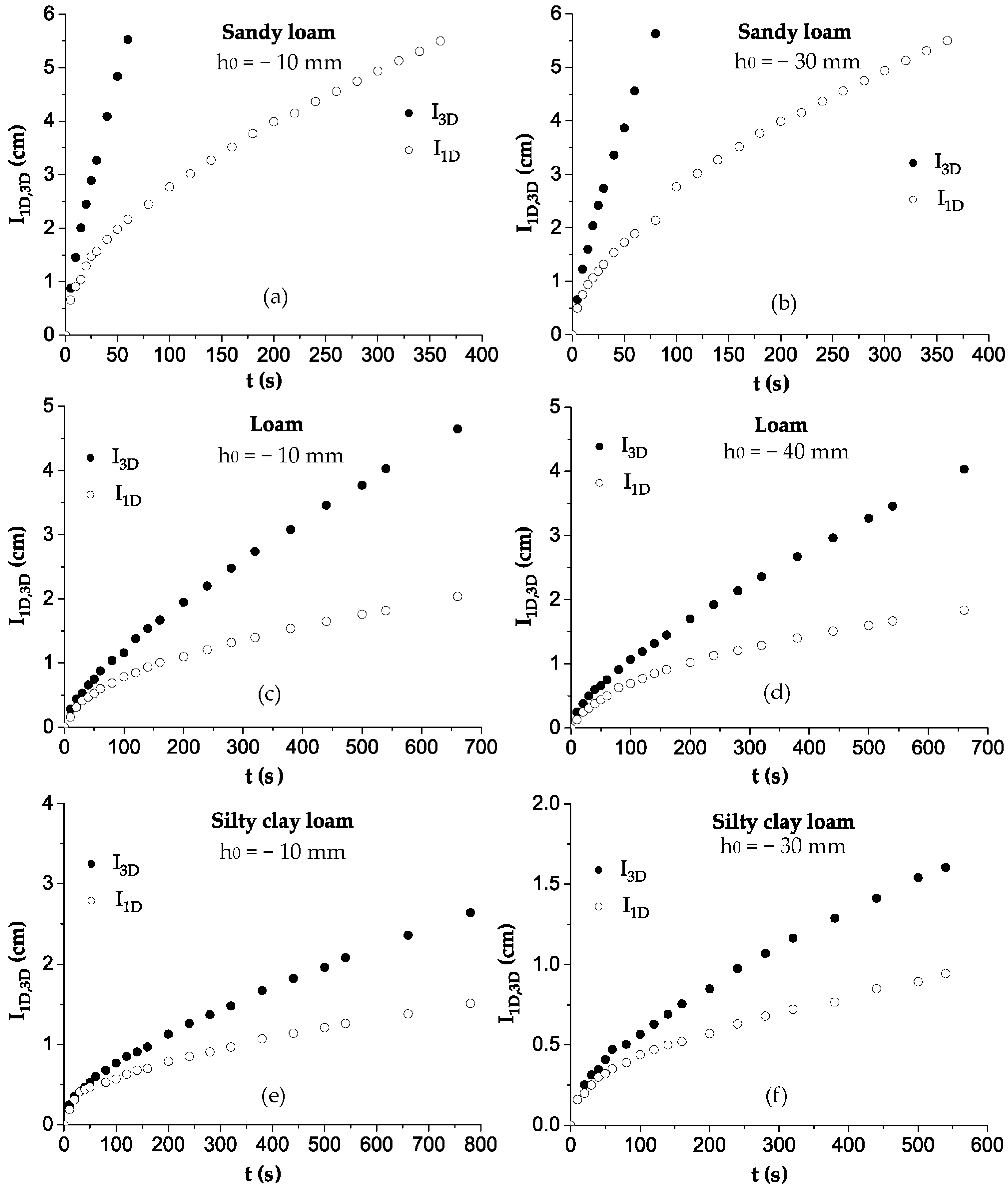
2.1. Three- and One-Dimensional Experiments Using the Mini Disc Infiltrometer

A mini disc infiltrometer [26] with a radius of 22.5 mm was used to perform three-dimensional infiltration experiments on repacked soils into a cylinder of 300 mm diameter and 300 mm length, and the disc was placed in the center at the soil surface to allow fully unconfined three-dimensional flow. On the other hand, one-dimensional infiltration experiments were performed on repacked soils into a cylinder of 45 mm diameter and 500 mm length, and the disc was placed on the top surface of the soils [27]. No contact material was required for these experiments.

The soils examined were a sandy loam, a loam, and a silty clay loam. The soil texture and the bulk density, ρ_φ, of soils are presented in

Table 1. Soil particle size distribution and bulk density, ρ_φ, of the soils examined.

Soil Type	Clay (%)	Silt (%)	Sand (%)	ρφ (g cm−3)
Sandy loam	13.2	8	78.8	1.41
Loam	20.0	38	42.0	1.17
Silty clay loam	36.5	52	11.5	1.23

. The disturbed soil samples used had been airdried and passed through a 2 mm sieve before the beginning of the experiments and, consequently, the initial soil water content was very low (θ_n = 0.04 cm³ cm⁻³ for all soils studied). The tested materials were carefully packed to a standard bulk density, as is shown in Table 1, for both cases of our experiments (three- and one-dimensional) for each soil tested. The pressure heads applied, during the three- and one-dimensional infiltration tests, were −30 and −10 mm for the sandy loam soil, −40 and −10 mm for the loam soil, and −30 and −10 mm for the silty clay loam soil. After cessation of each infiltration experiment, soil subsamples close to the surface were used for the determination of soil water content θ₀. The duration of the experiments ranged from 600 to 900 s. The experimental procedure we followed was similar to that of Smettem et al. (1994) [1].

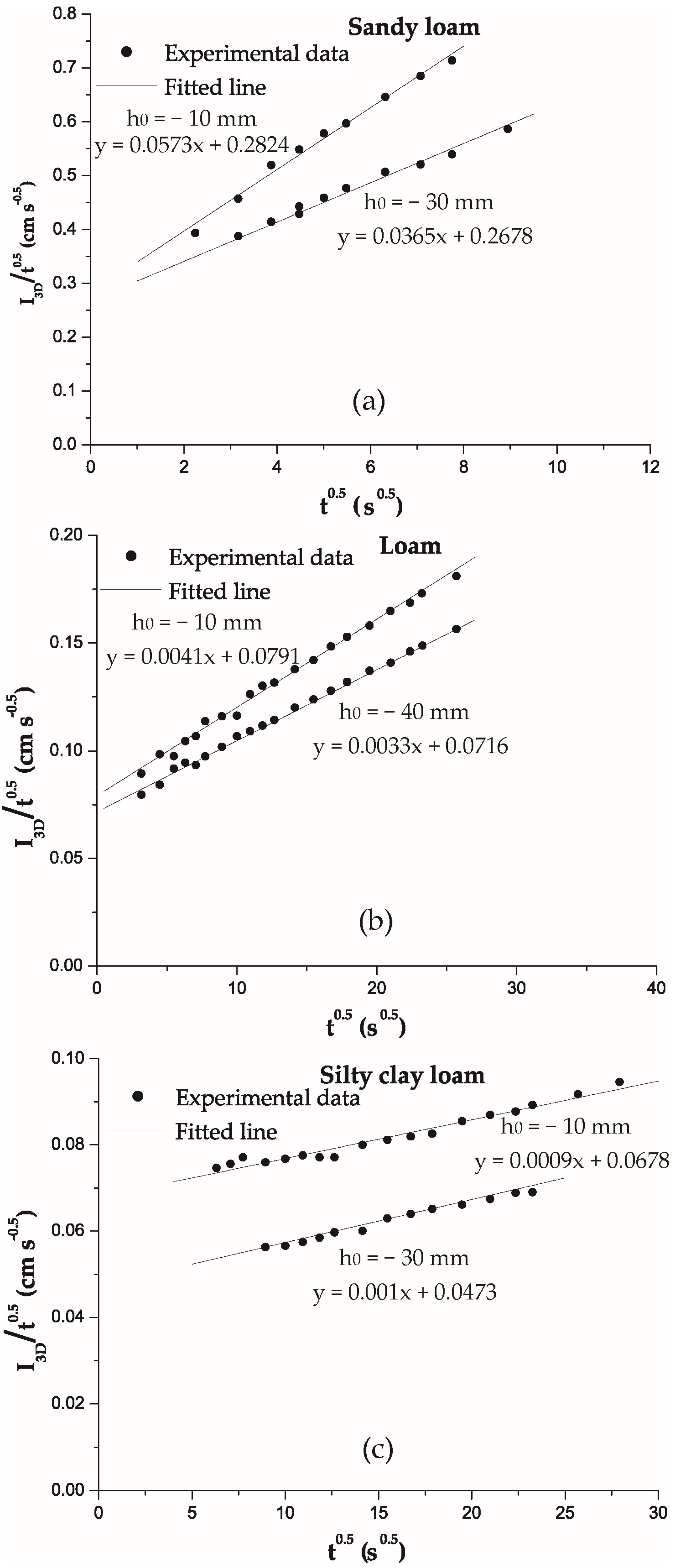
2.2. Estimation of Sorptivity

For the accurate estimation of γ from the difference of the three- and one-dimensional cumulative infiltration data (Equation (1)), an accurate determination of the sorptivity S₀ for every soil water pressure head imposed on the surface of each soil tested is needed. In this respect, the determination of the sorptivity S₀ was made according to two different ways. The sorptivity S₀ value for each pressure head h₀ was obtained from the slope of the one-dimensional infiltration data ${\mathrm{I}}_{1\mathrm{D}}$ as a function of $\sqrt{\mathrm{t}}$, for short times up to 60 s where the ${\mathrm{I}}_{1\mathrm{D}}\left(\sqrt{\mathrm{t}}\right)$ relationship is linear. In addition, an estimate of S₀ was also obtained from the intercept term of the three-dimensional infiltration data ${\mathrm{I}}_{3\mathrm{D}}/\left(\sqrt{\mathrm{t}}\right)$ as a function of $\sqrt{\mathrm{t}}$ (Equation (8)). The nonexistent difference of sorptivity S₀ between the two different methods is indirect evidence of the fact that the packing of the soil in the two methods was similar.

2.3. Determination of Soil Water Content

At the end of the three-dimensional infiltration experiment, a wet subsoil sample exactly below the mini disc infiltrometer was obtained and placed in an oven at 105 °C for 48 h in order to determine its gravimetric water content, w, according to the expression:

$$\mathrm{w}=\frac{{\mathrm{m}}_{\mathrm{w}}}{{\mathrm{m}}_{\mathrm{s}}}$$

(9)

where m_w the mass of water retained in the wet sample and m_s the mass of oven-dry soil (solid soil particles).

Knowing the bulk soil density ρ_φ, and density of water ρ_w, as:

$${\mathsf{\rho }}_{\mathsf{\phi }}={\mathrm{m}}_{\mathrm{s}}/{\mathrm{V}}_{\mathrm{o}}$$

(10)

$${\mathsf{\rho }}_{\mathrm{w}}={\mathrm{m}}_{\mathrm{w}}/{\mathrm{V}}_{\mathrm{w}}$$

(11)

where V_o the volume of the soil sample, then the volumetric water content θ₀ can be calculated from the combination of Equations (9)–(11) as follows:

$$\mathrm{w}=\frac{{\mathsf{\rho }}_{\mathrm{w}}{\mathrm{V}}_{\mathrm{w}}}{{\mathsf{\rho }}_{\mathsf{\phi }}{\mathrm{V}}_{\mathrm{o}}}=\frac{{\mathsf{\rho }}_{\mathrm{w}}}{{\mathsf{\rho }}_{\mathsf{\phi }}}{\mathsf{\theta }}_0\Rightarrow {\mathsf{\theta }}_0=\frac{{\mathsf{\rho }}_{\mathsf{\phi }}}{{\mathsf{\rho }}_{\mathrm{w}}}\mathrm{w}$$

(12)

3. Results and Discussion

3.1. Estimation of Sorptivity

In Figure 1, three- and one-dimensional cumulative infiltration versus time relationships are depicted for sandy loam, loam, and silty clay loam soils for each pressure head used.

The sorptivity S₀ can be calculated by the equation ${\mathrm{I}}_{3\mathrm{D}}={\mathrm{I}}_{1\mathrm{D}}={\mathrm{S}}_0\sqrt{\mathrm{t}}$ at short times ($\mathrm{t}\to 0$). However, Smettem et al. [10] and Minasny and McBratney [28] showed that the classical approach to calculating sorptivity from a disc infiltrometer experiment (three-dimensional infiltration flow) may give erroneous results (overestimated). For this reason, the S₀ value for each pressure head was obtained from the slope of the linear relationship of the one-dimensional infiltration data versus square root of time, ${\mathrm{I}}_{1\mathrm{D}}\left(\sqrt{\mathrm{t}}\right)$ (data not shown), for short times, where the effect of the gravity is negligible (

Table 2. One-dimensional infiltration parameters, h₀, θ₀, and S₀, for sandy loam, loam, and silty clay loam soil. R² is the coefficient of determination between the experimental infiltration data ${\mathrm{I}}_{1\mathrm{D}}\left(\sqrt{\mathrm{t}}\right)$ and fitted curve for S₀ estimation.

Soil Type	Pressure Head, h0 (mm)	Water Content, θ0 (cm3 cm−3)	Soil Sorptivity, S0 (cm s−0.5)	R2
Sandy loam	−10	0.399	0.284	0.997
	−30	0.385	0.241	0.999
Loam	−10	0.385	0.072	0.970
	−40	0.369	0.063	0.958
Silty clay loam	−10	0.464	0.061	0.990
	−30	0.446	0.046	0.990

).

The choice of the appropriate time interval for calculating S₀ in the one-dimensional infiltration experiments is relatively easy, since no sand layer is needed to be used on the surface of each porous medium to ensure hydraulic contact between the infiltrometer and the soil. The presence of this layer can be manifested on the first stages of infiltration, making the estimation of the appropriate time interval for calculating S₀ difficult [5,29].

Additionally, the value of S₀ at each pressure head was calculated by linearization of Equation (2) using the three-dimensional infiltration data. In Figure 2, the fitted curve of the linear relationship $\frac{\mathrm{I}}{\sqrt{\mathrm{t}}}={\mathrm{C}}_1+{\mathrm{C}}_2\sqrt{\mathrm{t}}$ on the three-dimensional infiltration data using various pressure heads, h₀, for all soils studied, are presented. As shown in Figure 2, from the fitting functions on three-dimensional infiltration data using Equation (8), the S₀ value, from the intercept term, can be obtained. The intercept values for all pressure heads tested in the three soils were very close to the S₀ values obtained from the slope of the linear relationship of the one-dimensional infiltration data versus square root of time, ${\mathrm{I}}_{1\mathrm{D}}\left(\sqrt{\mathrm{t}}\right)$, and are presented in Table 2. The same results came from Smettem et al. [10]. Perroux and White [30], after conducting disc infiltrometer experiments, showed that the time for estimating S₀ depends on the soil type and ranged from 6 to 2450 s, with an average value of 60 s. Vandervaere et al. [19] reported that a difference up to 15% between S₀ values obtained from three- and one-dimensional infiltration is acceptable due to possible different soil packing.

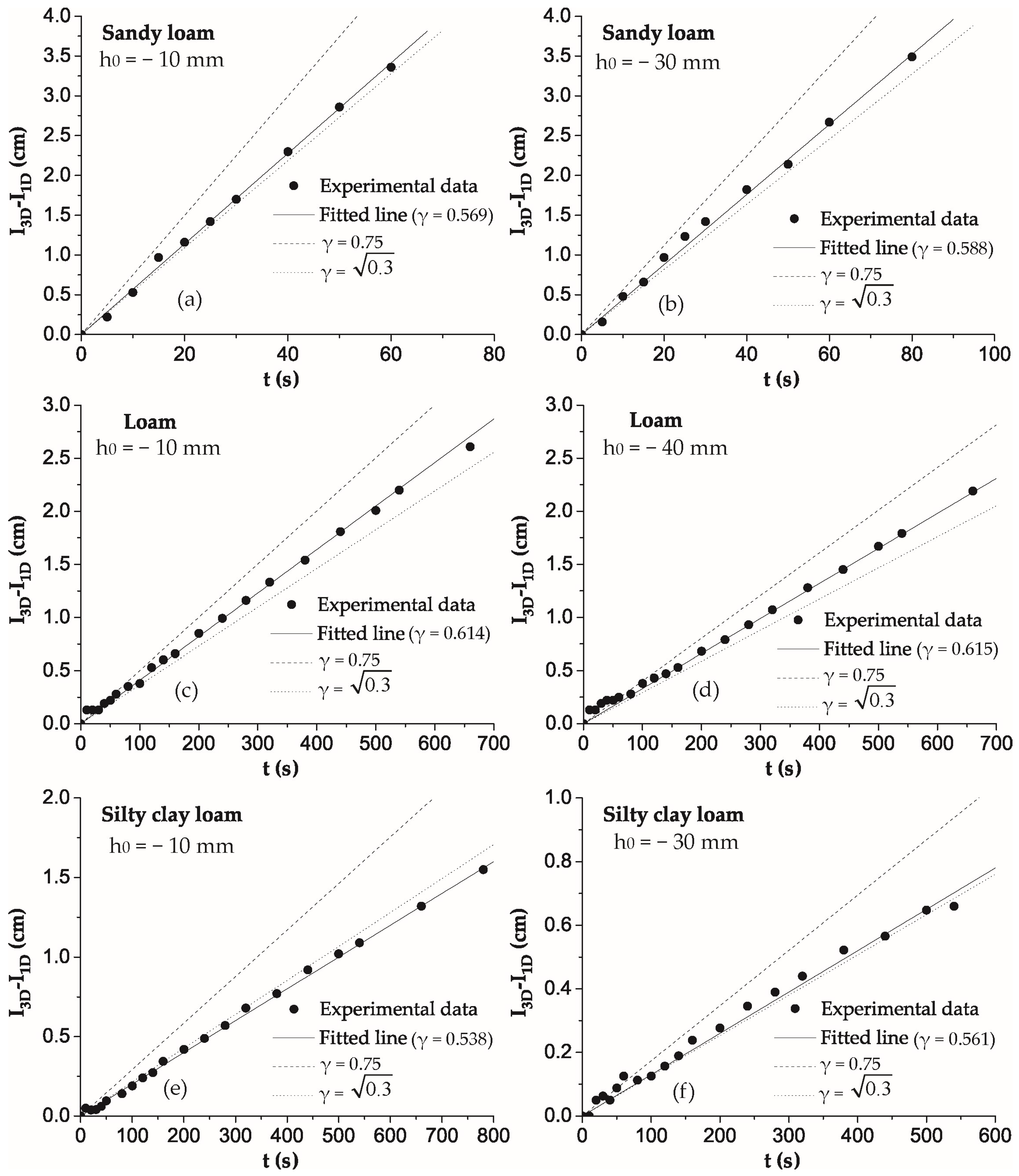
3.2. Estimation of Difference between Three- and One-Dimensional Infiltration Data

In Figure 3, the difference between experimental three- and one-dimensional cumulative infiltration (I_3D−I_1D) as a function of time t, for each pressure head tested in the three soils, is presented. As shown, the difference I_3D−I_1D is linear in time t for all cases studied, with a coefficient of determination R² > 0.98 (

Table 3. Estimated shape parameter γ from the slope of the fitted linear function I_3D−I_1D (t) on the experimental data using Equation (1). R² is the coefficient of determination between the experimental I_3D−I_1D (t) data and fitted curve for γ estimation.

Soil Type	Pressure Head, h0 (mm)	γ	Slope (cm min−1)	R2
Sandy loam	−10	0.569	0.0569	0.996
	−30	0.588	0.0440	0.996
Loam	−10	0.614	0.0041	0.998
	−40	0.615	0.0033	0.995
Silty clay loam	−10	0.538	0.0020	0.998
	−30	0.561	0.0013	0.989

), as predicted by Equation (1) of Smettem et al. [1], and independent of gravity. It also appears that the slope of this linear function decreases by reducing the pressure head (Table 3). This practically means that the reduction of S₀ is greater and predominant compared to the difference of soil water content θ₀−θ_n.

Moreover, in Figure 3, the difference between three- and one-dimensional cumulative infiltration (I_3D−I_1D) was presented for two different values of shape parameter γ ($\sqrt{0.3}$ and 0.75). The comparison between the experimental relationship I_3D−I_1D (t) and the predicted one by Equation (1) (using the S₀ and θ₀ values presented in Table 2) showed a good agreement with the shape parameter γ = $\sqrt{0.3}$, for all porous media used (Figure 3). This could be anticipated, since the experimental γ values are very close to the value $\sqrt{0.3}$, as was shown in both Table 3 and Figure 3.

In other words, the slope of experimental I_3D−I_1D as a function of time t was smaller than that obtained from Equation (1) using γ = 0.75. The values of γ which resulted from the mini disc infiltrometer seem to be close to the values of γ which were obtained through the application of the equation of Fuentes et al. (1992) [13] and were presented by Lassabatere et al. (2007) [11] for four soils using a disc infiltrometer of radius r = 10 cm. Moreover, it is shown that for this group of soils the values of γ are not seriously affected by the soil type. Nonetheless, a lot more experiments using more different soils are needed in order to reach safer conclusions. The difference between the experimental values of γ of our study (Table 3) and those ones are referred in the works of Haverkamp et al. [4], Smettem et al. [10], and Lassabatere et al. (2007) [11] may be attributed to various factors, such as initial conditions, as well as radius of infiltrometer. Haverkamp et al. (2005) [31] have reported the effect of initial water content on the shape parameter γ value, while Warrick and Lazarovitch (2007) [12] reported that the value of γ depends on the geometry of the infiltration source.

3.3. Effect of γ Parameter to Hydraulic Conductivity Calculation

It is profound that the smaller values of γ obtained for the case of the mini disc infiltrometer would reflect on the validity of the criteria (Equations (6) and (7)) for the possibility of the calculation of K₀ from Equation (5), since smaller values of γ will make it more probable that Equations (6) and (7) are valid. It is worth noting that neither the criterion to check K₀ calculation reliability of Vandervaere et al. [19] (Equation (6)) nor that of Dohnal et al. [24] (Equation (7)) is fulfilled in all cases of soils examined when γ = 0.75. In other words, K₀ is a minor term in C₂ (Equation (5)) and consequently, the K₀ estimate is unreliable. However, the smaller values of γ which were determined in the soils examined increases the possibility of reliable K₀ values calculation, since the criterion of Dohnal et al. [24] is more likely to be fulfilled.

In the cases of the sandy loam soil, at pressure head −10 mm, and loam soil, at pressure heads −10 and −40 mm, the criterion of Dohnal et al. [24] was fulfilled using the value of γ = $\sqrt{0.3}$, giving reliable K₀ values (0.34, 0.057, and 0.046 cm min⁻¹, respectively). On the other hand, the aforementioned criterion is not fulfilled in the case of the silty clay loam soil using this γ value. In this soil (fine-textured), the lateral capillary flow is of overwhelming importance [24].

4. Conclusions

The difference between experimental three- and one-dimensional cumulative infiltration data of three soils using a mini disc infiltrometer is linearly proportional to time. However, the shape parameter γ is different from that calculated by other researchers who conducted experiments on different soils using different infiltrometers. Additionally, from the three soils under the present investigation, it is shown that the value of γ is not seriously affected by the soil type. The calculation of the γ value, in combination with the value of S₀, as calculated by various methodologies, can be used to calculate the contribution of gravitational flow during three-dimensional infiltration. However, in fine-textured soils with strong lateral capillary flow, the calculation of K₀ is still unreliable.

References

1. Smettem, K.R.J.; Parlange, J.Y.; Ross, P.J.; Haverkamp, R. Three-dimensional analysis of infiltration from the disc infiltrometer: 1. A capillary-based theory. Water Resour. Res. 1994, 30, 2925–2929. [Google Scholar] [CrossRef] [Green Version]
2. Smettem, K.R.J.; Clothier, B.E. Measuring unsaturated sorptivity and hydraulic conductivity using multiple disc permeameters. J. Soil Sci. 1989, 40, 563–568. [Google Scholar] [CrossRef]
3. Warrick, A.W. Models for disc infiltrometers. Water Resour. Res. 1992, 28, 1319–1327. [Google Scholar] [CrossRef]
4. Haverkamp, R.; Ross, P.J.; Smettem, K.R.J.; Parlange, J.Y. Three dimensional analysis of infiltration from disc infiltrometer: 2. Physically-based infiltration equation. Water Resour. Res. 1994, 30, 2931–2935. [Google Scholar] [CrossRef]
5. Vandervaere, J.P.; Vauclin, M.; Elrick, D.E. Transient flow from tension infiltrometers: I. The two parameter equation. Soil Sci. Soc. Am. J. 2000, 64, 1263–1272. [Google Scholar] [CrossRef]
6. Smettem, K.R.J. Characterization of water entry into a soil with a contrasting textural class: Spatial variability of infiltration parameters and influence of macroporosity. Soil Sci. 1987, 144, 167–174. [Google Scholar] [CrossRef]
7. Mohanty, B.P.; Ankeny, M.D.; Horton, R.; Kanwar, R.S. Spatial analysis of hydraulic conductivity measured using disc infiltrometers. Water Resour. Res. 1994, 30, 2489–2498. [Google Scholar] [CrossRef]
8. Shouse, P.J.; Mohanty, B.P. Scaling of near-saturated hydraulic conductivity measured using disc infiltrometers. Water Resour. Res. 1998, 34, 1195–1205. [Google Scholar] [CrossRef] [Green Version]
9. Quadri, M.B.; Angulo-Jaramillo, R.; Vauclin, M.; Clothier, B.E.; Green, S.R. Axisymmetric transport of water and solute underneath a disk permeameter: Experiments and numerical model. Soil Sci. Soc. Am. J. 1994, 58, 696–703. [Google Scholar] [CrossRef]
10. Smettem, K.R.J.; Ross, P.J.; Haverkamp, R.; Parlange, J.Y. Three-dimensional analysis of infiltration from the disc infiltrometer: 3. Parameter estimation using a double-disk tension infiltrometer. Water Resour. Res. 1995, 31, 2491–2495. [Google Scholar] [CrossRef]
11. Lassabatere, L.; Angulo-Jaramillo, R.; Soria-Ugalde, J.M.; Simunek, J.; Haverkamp, R. Numerical evaluation of a set of analytical infiltration equations. Water Resour. Res. 2009, 45, W12415. [Google Scholar] [CrossRef]
12. Warrick, A.W.; Lazarovitch, N. Infiltration from a strip source. Water Resour. Res. 2007, 43, W03420. [Google Scholar] [CrossRef]
13. Fuentes, C.R.; Haverkamp, R.; Parlange, J.Y. Parameter constraints on closed-form soil water relationships. J. Hydrol. 1992, 137, 117–142. [Google Scholar] [CrossRef]
14. Warrick, A.W.; Lazarovitch, N.; Furman, A.; Zcrihun, D. Explicit infiltration function for furrows. J. Irrig. Drain. Eng. 2007, 133, 307–313. [Google Scholar] [CrossRef]
15. Clothier, B.E.; White, I. Measurement of sorptivity and soil water diffusivity in the field. Soil Sci. Soc. Am. J. 1981, 45, 241–245. [Google Scholar] [CrossRef]
16. Ankeny, M.D.; Ahmed, Μ.; Kaspar, T.C.; Horton, R. Simple field method for determining unsaturated hydraulic conductivity. Soil Sci. Soc. Am. J. 1991, 55, 467–470. [Google Scholar] [CrossRef]
17. Reynolds, W.D.; Elrick, E.D. Determination of hydraulic conductivity using a tension infiltrometer. Soil Sci. Soc. Am. J. 1991, 55, 633–639. [Google Scholar] [CrossRef]
18. Zhang, R. Infiltration models for the disc infiltrometer. Soil Sci. Soc. Am. J. 1997, 61, 1597–1603. [Google Scholar] [CrossRef]
19. Vandervaere, J.P.; Vauclin, M.; Elrick, D.E. Transient flow from tension infiltrometers: II. Four methods to determine sorptivity and conductivity. Soil Sci. Soc. Am. J. 2000, 64, 1272–1284. [Google Scholar] [CrossRef]
20. Latorre, B.; Moret-Fernández, D.; Peña, C. Estimate of soil hydraulic properties from disc infiltrometer three-dimensional infiltration curve: Theoretical analysis and field applicability. Procedia Environ. Sci. 2013, 19, 580–589. [Google Scholar] [CrossRef]
21. Wooding, R.A. Steady infiltration from shallow circular pond. Water Resour. Res. 1968, 4, 1259–1273. [Google Scholar] [CrossRef]
22. Vandervaere, J.P. The soil solution phase. In Methods of Soil Analysis: Part 4, Physical Methods; Dane, J.H., Topp, G.C., Eds.; Soil Science Society of America (SSSA, Inc.): Madison, WI, USA, 2002; pp. 889–894. [Google Scholar]
23. Philip, J.R. The theory of infiltration: 4. Sorptivity and algebraic infiltration equations. Soil Sci. 1957, 84, 257–264. [Google Scholar] [CrossRef]
24. Dohnal, M.; Dusek, J.; Vogel, T. Improving hydraulic conductivity estimates from mini disk infiltrometer measurements for soils with wide pore-size distributions. Soil Sci. Soc. Am. J. 2010, 74, 804–811. [Google Scholar] [CrossRef]
25. Smiles, D.E.; Knight, J.H. A note on the use of the Philip infiltration equation. Aust. J. Soil Res. 1976, 14, 103–108. [Google Scholar] [CrossRef]
26. Decagon Devices. Mini Disc Infiltrometer, User’s Manual; Decagon Devices Inc.: Pullman, DC, USA, 2007. [Google Scholar]
27. Kargas, G.; Londra, P.; Anastasiou, K. Investigation of the relationship between three- and one-dimensional infiltration using a mini disc infiltrometer. In Proceedings of the 3rd EWaS International Conference on “Insights on the Water-Energy-Food Nexus”, Lefkada Island, Greece, 27–30 June 2018. [Google Scholar]
28. Minasny, B.; McBratney, A.B. Estimation of sorptivity from disc-permeameter measurements. Geoderma 2000, 95, 305–324. [Google Scholar] [CrossRef]
29. Vandervaere, J.P.; Peugeot, C.; Vauclin, M.; Angulo-Jaramillo, R.; Lebel, T. Estimating hydraulic conductivity of crusted soils using disc infiltrometers and minitensiometers. J. Hydrol. 1997, 188–189, 203–223. [Google Scholar] [CrossRef]
30. Perroux, K.M.; White, I. Designs for disc permeameters. Soil Sci. Soc. Am. J. 1988, 52, 1205–1215. [Google Scholar] [CrossRef]
31. Haverkamp, R.; Debionne, D.; Viallet, P.; Angulo-Jaramillo, R.; de Condapa, D. Soil properties and moisture movement in the unsaturated zone. In The Handbook of Groundwater Engineering; Delleur, J.W., Ed.; CRC Press: Boca Raton, FL, USA, 2005; pp. 1–59. [Google Scholar]
Figure 1. Representation of three- and one-dimensional experimental cumulative infiltration data with time, I1D,3D(t), for various pressure heads: (a) h0 = −10 mm and (b) h0 = −30 mm for sandy loam soil; (c) h0 = −10 mm and (d) h0 = −40 mm for loam soil; and (e) h0 = −10 mm and (f) h0 = −30 mm for silty clay loam soil.
Water 10 01783 g001
Figure 2. Linear representation of three-dimensional experimental infiltration data and fitted linear lines for various pressure heads, h0, for (a) sandy loam, (b) loam, and (c) silty clay loam soil.
Water 10 01783 g002
Figure 3. The difference between experimental three- and one-dimensional cumulative infiltration over time, for pressure heads: (a) h0 = −10 mm and (b) h0 = −30 mm for sandy loam soil; (c) h0 = −10 mm and (d) h0 = −40 mm for loam soil; and (e) h0 = −10 mm and (f) h0 = −30 mm for silty clay loam soil. The experimental γ value was calculated from the slope of the fitted line (solid line) using Equation (1). The model lines are derived from Equation (1) using two different values of γ: (i) 0.3 (dotted line) and (ii) 0.75 (dashed line).
Water 10 01783 g003