Article

Numerical Investigations of Tsunami Run-Up and Flow Structure on Coastal Vegetated Beaches

1
School of Ocean Science and Environment, Dalian Ocean University, Dalian 116023, China
2
State Key Laboratory of Coastal and Offshore Engineering, Dalian University of Technology, Dalian 116023, China
*
Author to whom correspondence should be addressed.
Water 2018, 10(12), 1776; https://doi.org/10.3390/w10121776
Submission received: 23 October 2018 / Revised: 28 November 2018 / Accepted: 29 November 2018 / Published: 3 December 2018
(This article belongs to the Special Issue Ocean Exchange and Circulation)

Abstract

:
Tsunami waves become hazardous when they reach the coast. In South and Southeast Asian countries, coastal forest is widely utilized as a natural approach to mitigate tsunami damage. In this study, a depth-integrated numerical model was established to simulate wave propagation in a coastal region with and without forest cover. This numerical model was based on a finite volume Roe-type scheme, and was developed to solve the governing equations with the option of treating either a wet or dry wave front boundary. The governing equations were modified by adding a drag force term caused by vegetation. First, the model was validated for the case of solitary wave (breaking and non-breaking) run-up and run-down on a sloping beach, and long periodic wave propagation was investigated on a partially vegetated beach. The simulated results agree well with the measured data. Further, tsunami wave propagation on an actual-scale slope covered by coastal forest Pandanus odoratissimus (P. odoratissimus) and Casuarina equisetifolia (C. equisetifolia) was simulated to elucidate the influence of vegetation on tsunami mitigation with a different forest open gap. The numerical results revealed that coastal vegetation on sloping beach has significant potential to mitigate the impacts from tsunami waves by acting as a buffer zone. Coastal vegetation with open gaps causes the peak flow velocity at the exit of the gap to increase, and reduces the peak flow velocity behind the forest. Compared to a forest with open gaps in a linear arrangement, specific arrangements of gaps in the forest can increase the energy attenuation from tsunami wave. The results also showed that different cost-effective natural strategies in varying forest parameters including vegetation collocations, densities, and growth stages had significant impacts in reducing the severity of tsunami damage.

1. Introduction

Tsunamis are generated by marine earthquakes, underwater volcanic eruptions, or submerged landsides. Recent tsunami disasters (e.g., in the Indian Ocean in 2004, Samoa in 2009, Chile in 2010, Tohoku in 2011, and Indonesia in 2018) have caused vast losses of life and property, destruction of critical infrastructure in low-lying coastal areas, and massive damage to the coastal ecosystem [1,2,3,4]. These great threats demonstrate the need to mitigate tsunamis by using artificial obstacles including wave-dissipating blocks, rock breakwaters, and large embankments. Recent studies investigated tsunami waves in both laboratory experiments [5,6,7,8] and field investigations [9,10] with the ultimate goal of mitigating their impacts and reducing natural disasters in coastal regions. Considering the advantages of flexibility and repeatability in numerical models, many numerical simulations have been carried out using different models to investigate the run-up heights and velocity processes of tsunamis [11,12,13,14,15,16]. Typical models that were considered included depth-integrated Boussinesq-type models and depth-integrated non-linear shallow water models (NSWMs), with results showing that NSWMs are more robust and efficient for tsunami predictions in real-scale basins.
Generally, coastal forests which act as natural obstacles are widely distributed in coastal areas. They also effectively mitigate tsunami damage from economic, environmental, and aesthetically pleasing points of view in concert with hard structures [17,18]. Currently, there is some literature on the capability of coastal vegetation to attenuate wave energy in short-period waves [19,20]. While tsunamis are categorically different from short-period waves, there have been an increasing number of studies that address the role of vegetation in mitigating coastal natural disasters, which can include the strategy of planting coastal vegetation as a bio-shield [21,22,23]. Recent research has calculated the friction and drag force of vegetation in a tsunami, using mathematical equations. Real-scale simulations of tsunami were performed to investigate the effectiveness of forests as a bio-shield for tsunami protection, with results indicating that a forest with two layers in the vertical direction including P. odoratissimus and C. equisetifolia was effective for attenuating the wave energy [24]. Based on two dimensional nonlinear long-wave equations, Thuy et al. developed a numerical model to estimate tree-breaking, the drag forces, and turbulence-induced shear force due to the presence of vegetation (P. odoratissimus and C. equisetifolia) [25]. Considering the effects of the porosity of vegetation, a one-dimensional numerical model using Boussinesq-type equations was developed to evaluate the effects of the forest density distribution on tsunami-force reduction, including the drag and inertia forces caused by vegetation [26]. Numerical investigations were conducted to study the impact of patchy vegetation on tsunami dynamics based on Boussinesq model, and the results demonstrated that patchy vegetation, with appropriate configuration, can be effective in mitigating tsunami hazards [27]. Based on a nonlinear long wave equation model that included the breaking or washout of trees, numerical simulations were carried out to estimate the effects of coastal forest and sea embankments on reducing the washout area and the tsunami mitigation function of the coastal forest [28].
Roads are perpendicular to the coast function as pathways that form gaps in the vegetation of the coastal forest. Gaps in the coastal forest can increase risks and potential damage, as the water flow from the tsunami accelerates as it moves through the gap into the densely populated block [29]. Tanimoto et al. studied it by changing the width of open gap and found that a specific gap with 15 m width causes the highest flow velocity in their simulated conditions [30]. Thuy et al. numerically simulated the effect of an open gap in coastal forests on tsunami run-up, and found that maximum flow velocity greatly increased at the open gap exit, meaning that an open gap (like a road) in a coastal forest had a negative effect on tsunami run-up behind the forest [31]. Nandasena et al. investigated hydrodynamic parameters (flow velocity and depth) of tsunami waves and bending moment of vegetation on Misawa, a site covered by pine forest with two gaps [32]. However, no studies have discussed the effects of different open gaps in existing forests via the analysis of maximum tsunami run-up and variations of velocity through the gaps using a model with shock capture capability.
In this paper, we numerically investigate the hydrodynamic processes on a vegetated sloping beach and quantify the effects of a gap in forest vegetation on the run-up by solving the depth-averaged 2D model. The proposed model was tested for breaking and non-breaking solitary waves propagating on a bare sloping beach, and long periodic wave propagation on a partially-vegetated sloping beach to examine the accuracy of the numerical model. Then, the model was used to simulate tsunami waves propagating on actual-scale forest-covered beach, and to study the mitigation effects of gap arrangements and different vegetation parameters on tsunami waves.

2. Numerical Method

2.1. Governing Equations

The depth-averaged 2D shallow water equations are formed by integrating the Navier–Stokes equations which include continuity and momentum equations for depth-averaged free surface flows. These are expressed as Equations (1)–(3):
h t + u h x + v h y = 0
h u t + ( h u u ) x + ( h u v ) y x ( v t h u x ) y ( v t h u y ) = g h η x τ b x + f c h v f x
h v t + ( h u v ) x + ( h v v ) y x ( v t h v x ) y ( v t h v y ) = g h η y τ b y f c h u f y
In the above equations, t is time, h indicates the local water depth, u and v stand for the depth-averaged flow velocities in the x and y directions, respectively, η stands for the water surface elevation from a reference datum, vt is defined as the eddy viscosity coefficient calculated by ν t = α u h where α is empirical constant and ranges from 0.3 to 1.0, u means the bed shear velocity, τ b x and τ b y denote friction in the x and y directions, respectively, τ b x = g n 2 u u 2 + v 2 h 1 3 , τ b y = g n 2 v u 2 + v 2 h 1 3 , where n stands for Manning’s roughness coefficient, fc indicates the Coriolis parameter, and fx and fy stand for the drag force caused by vegetation.
The conservative and vector form of 2D shallow water equations with vegetation effects are expressed as follows:
U t + F x + G y = F d x + G d y + S
The definitions of U, F, G, Fd and Gd are shown as follows:
U = [ h h u h v ] , F = [ h u h u u h u v ] , G = [ h v h u v h v v ] , F d = [ 0 ν t u h x ν t v h x ] , G d = [ 0 ν t u h y ν t v h y ] , S = [ 0 g h η x τ b x + f c h v f x g h η y τ b y f c h u f y ]
For notational convenience, Equation (4) is often rewritten as:
U t + E w a d v = E w d i f + S
where E w a d v = F i + G j and E w d i f = F d i + G d j .

2.2. Vegetation Drag Force

The resistance effects of vegetation on flow are added into the momentum equations as an internal source of resistant force per unit fluid mass. The drag force exerted by vegetation per unit volume is expressed as [33]:
f x = 1 2 N C D ( h ) b v min ( h v , h ) u u 2 + v 2 , f y = 1 2 N C D ( h ) b v min ( h v , h ) v u 2 + v 2
Here, N stands for the vegetation density defined as the number of plants per square meter, bv indicates the diameter, and hv indicates the height of the vegetation. CD (h) indicates the depth-averaged equivalent drag coefficient which considers the vertical stand structures of a tree, defined by Tanaka et al. [1] as follows:
C D ( h ) = C D r e f 1 h 0 h α ( z g ) β ( z g ) d z g
α ( z g ) = b ( z g ) b r e f
β ( z g ) = C D ( z g ) C D - r e f
where CD-ref is the reference drag coefficient of the trunk at zg (equal to 1.2 m in principle), α(zg) is considered as an additional coefficient to express the effects of cumulative width on drag force at each height zg, b(zg) means the projected width, and bref indicates the reference projected width. β(zg) is expressed as an additional coefficient representing the effect of leaves or aerial roots on drag force, and CD(zg) is drag coefficient of a tree at the height zg above the ground surface.

2.3. Finite Volume Method

The discretization of the governing equations is based on the finite volume method using an unstructured triangular mesh. The conserved variables are defined at the cell centers and represent the average value of each cell. The integral form of Equation (10) over the ith control volume can be expressed as:
V i U t d V + V i E w a d v d V = V i E w d i f d V + V i S d V
In this expression, subscript i and j denote the element and the element side, respectively, while Vi stands for the domain of the ith. Basing Green’s theorem. Equation (11) can be rewritten as:
Δ U i Δ t A i = L i E w a d v n d l + L i E w d i f n d l + V i S d V
where U i stands for the average value of the conserved variables over the ith cell, and U i is stored at the center of the ith cell, with U i = 1 A i V i U d V . Li means the boundary of the Vi. A i denotes the area of the ith cell, n is the outward surface normal vector of Li, with n = ( n x , n y ) = ( cos ϕ , sin ϕ ) , and ϕ is the angle included between the x direction and the outward normal vector.
In the 2D triangular grid system, the line integral term in the Equation (12) can be further approximated and assessed as follows:
Δ U i = Δ t A i j = 1 m ( E w a d v n i j ) l i j + Δ t A i j = 1 m ( E w d i f n i j ) l i j + Δ t A i V i S d V
where m denotes the number of total edges of the triangular cell (three in this model), the subscript j means the index of the edge of a triangular mesh, n i j stands for the outward normal flux vector, and l i j means the length of the arc.

2.4. Evaluation of Numerical Fluxes

Variables are usually approximated as constant states within each control volume. Riemann problems at the interface of the cell can be solved using various Riemann approximations for evaluating the interface fluxes. The interface fluxes of Roe’s solver are expressed as follows:
E w a d v n = 1 2 [ ( F , G ) R n + ( F , G ) L n | J | ( U R U L ) ]
where U R and U L are reconstructed Riemann state variables on the right and left sides of the cell interface, respectively. The flux Jacobian matrix A can be assessed as:
| J | = ( E w a d v n ) U = F U n x + G U n y = [ 0 n x n y ( c 2 u 2 ) n x u v n y 2 u n x + v n y u n y u v n x + ( c 2 v 2 ) n y v n x u n x + 2 v n y ]
where n x and n y denote the components of the outward surface normal vector in the x- and y- directions, respectively, and c indicates the wave velocity, with
c = g h
where | J | = R | Λ | L , R and L stand for the right and left eigenvector matrices, and | Λ | denotes the diagonal matrix of the absolute values of the eigenvalues of A.
Where | Λ | is defined as:
| Λ | = ( Λ 1 0 0 0 Λ 2 0 0 0 Λ 3 )
where
λ 1 = u n x + v n y ,   λ 2 = u n x + v n y c ,   λ 3 = u n x + v n y + c
The right and left eigenvector matrices are expressed as follows:
R = ( 0 1 1 n y u c n x u + c n x n x v c n y v c n y ) ,   L = ( ( u n y v n x ) n y n x u n x + v n y 2 c + 1 2 n x 2 c n y 2 c u n x + v n y 2 c + 1 2 n x 2 c n y 2 c )
where the Riemann state variables u, v, and c on the cell interface are necessary to deal with the fluxes as calculated by Roe’s average:
u = h + u + + h u h + + h ,   v = h + v + + h v h + + h ,   c = g ( h + + h ) 2
The subscripts + and indicate the right and left sides of the cell edge, respectively. When the drying-wetting interfaces exist in the computational domain, Roe’s average can be calculated by: u = u + + u 2 , v = v + + v 2 .

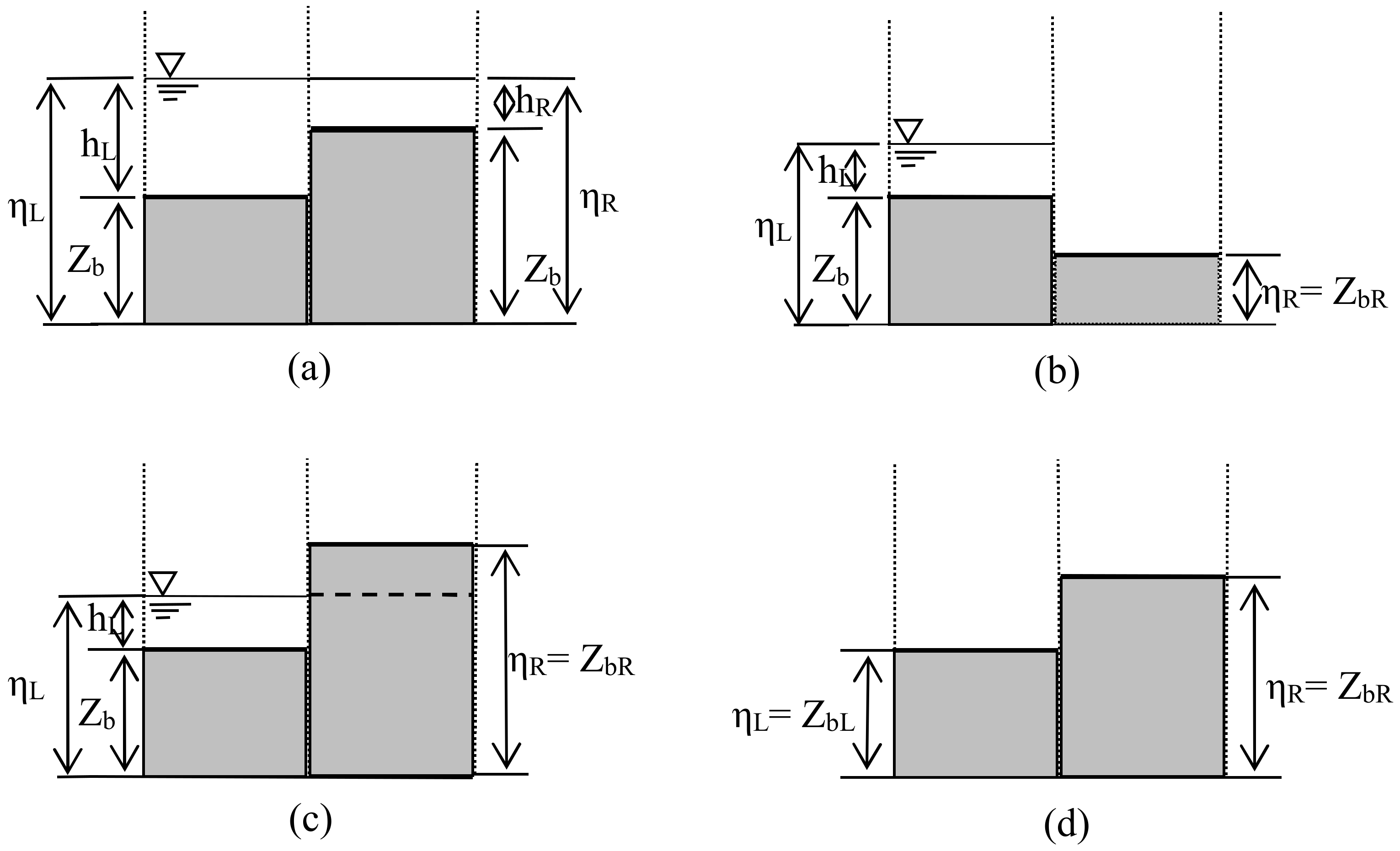
2.5. Treatment of Wetting and Drying Fronts

A technique to treat both wet and dry boundaries was introduced to achieve zero mass error [34,35]. A criterion, ε, was adopted to define and classify the following four types of edges:
  • Wet edge (see Figure 1a): two adjacent cells are wet, in which water depth of left cell hL > ε and water depth of right cell hR > ε.
  • Partially wet edge (with flux), as presented in Figure 1b: a wet cell (left) links to a dry cell on the right, and the water level of the wet cell is higher than that of the dry cell, where hL > ε, hR ≤ ε and water level of left cell ηL > water level of left cell ηR.
  • Partially wet edge (no flux), as shown in Figure 1c: a wet cell (left) links to a dry cell on the right, and the water level of the wet cell is lower than that of the dry cell, where hL > ε, hR ≤ ε, and ηL < ηR. To eliminate the non-physical flux problem produced in the interface, the water level ηR and bed level ZbR for the dry cell were temporarily replaced by a value which equaled to the water level ηL in the wet cell.
  • Dry edge, as presented in Figure 1d: two adjacent cells are dry, where hL ≤ ε and hR ≤ ε.
According to these four types of edges, cells were correspondingly divided into three types:
  • Wet cell: all the edges of this cell consisted of a wet or partially wet edges (with flux) and all the nodes of the cell are flooded.
  • Dry cell: all the edges of this cell consist of dry or partially wet edges (no flux).
  • Partially wet cell: all other cells do not satisfy the criteria of either a wet or dry cell, as defined above.

3. Numerical Simulation and Experimental Validation

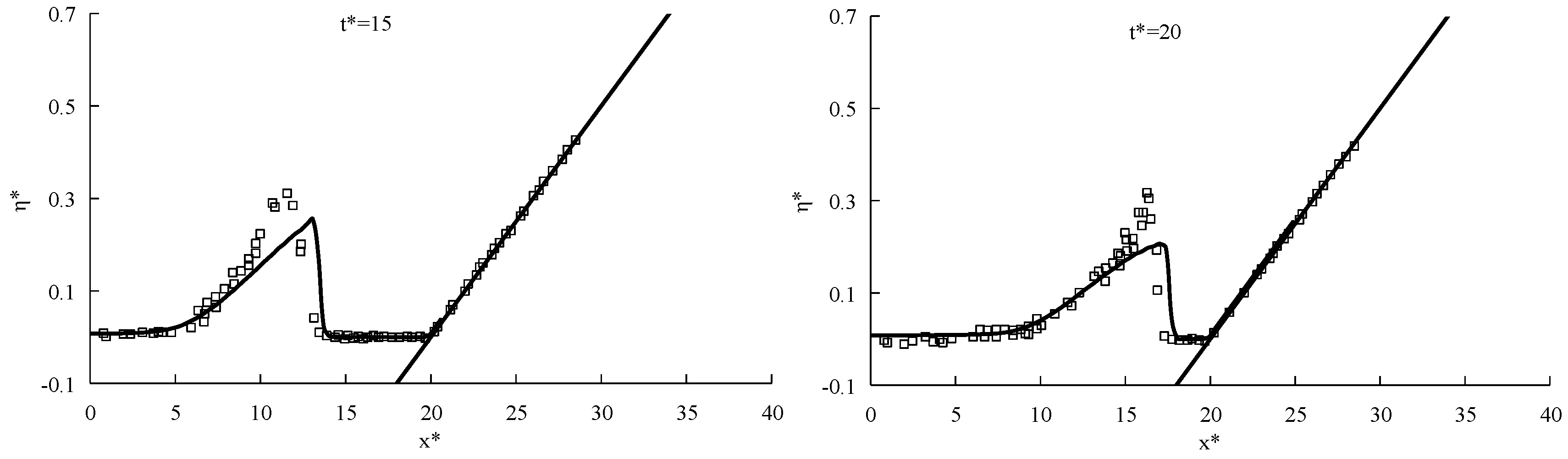
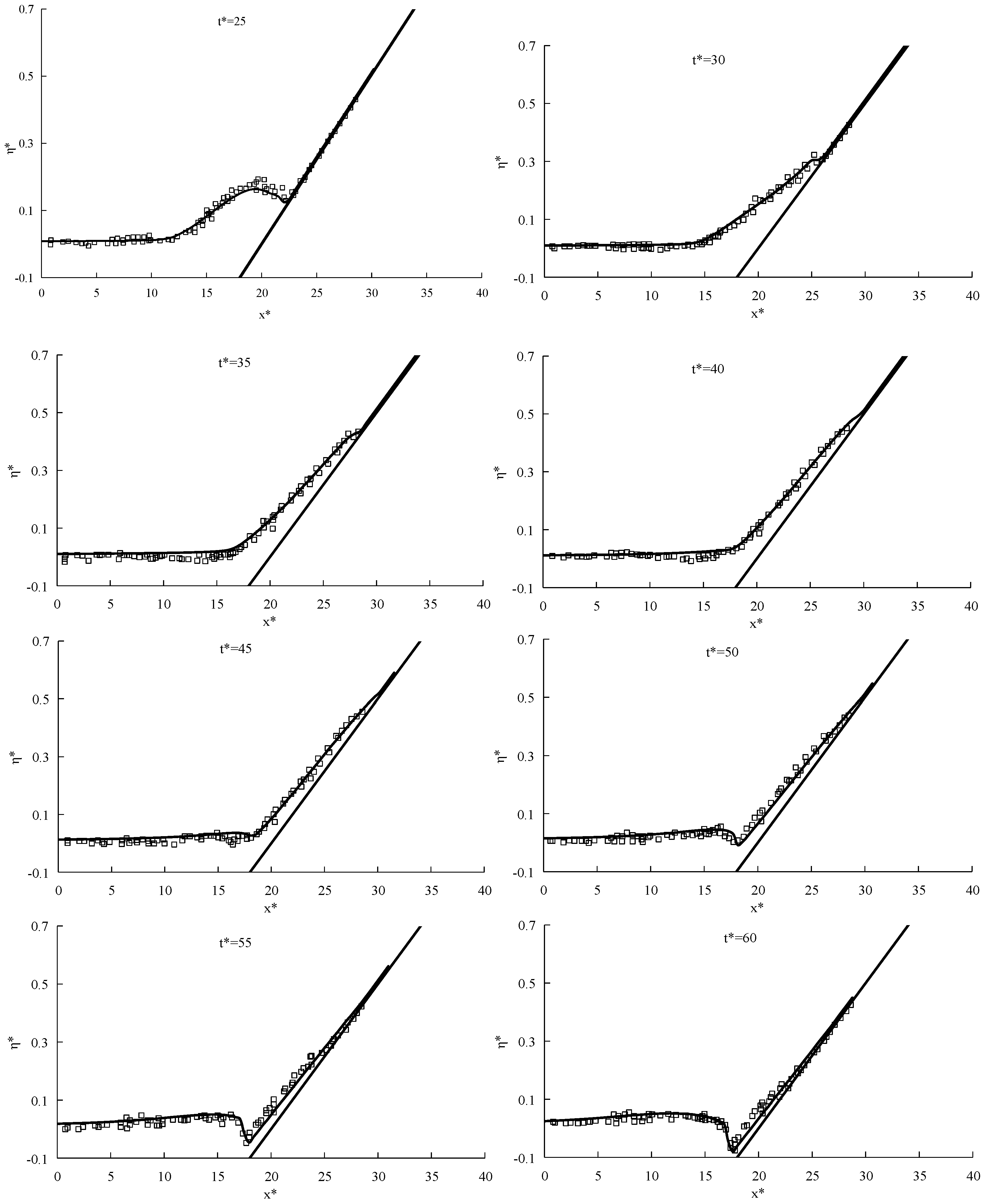
3.1. Solitary Wave Run-up on a Bare Sloping Beach

The depth-integrated shallow water model was run for experiment cases of breaking and non-breaking solitary waves on a bare sloping beach conducted by Synolakis to validate the accuracy of the numerical scheme for modeling wave run-up and run-down [36]. The topography consists of a 1:19.85 sloping beach adjacent to a constant depth region, as illustrated in Figure 2. A solitary wave propagates from left to right in a wave flume; and according to first-order solitary wave theory, the water surface elevation and velocity in initial time are defined as follows:
η ( x ) = H W sec h 2 ( 3 H W 4 h 0 3 ( x X 0 ) )
u ( x ) = η ( x ) g h 0
where Hw means wave height, h0 denotes initial water depth with a value of 1 m, X0 stands for the position of initial wave crest and is located a half wave length from the toe of the sloping beach in the computing domain, and u is wave velocity.
In this case study, the numerical model used uniform triangular cells with a grid spacing of 0.02 m and a time step of 0.001 s. The minimum water depth to define a “dry bed” was set as 0.0001 m, and the Manning’s bed roughness coefficient was calibrated as 0.01 for the glassed flume in the present model. The solitary wave was defined as non-breaking in this case, as Hw/h0 = 0.0185. For convenience, the results are presented in non-dimensional forms: x = x h 0 , η = η h 0 and t = t g h 0 . Comparisons of the simulated and experimental free-surface evolutions are presented in Figure 3. As illustrated, the incident wave propagates on the sloping beach at the early stage (t = 25, 30, 35, 40, 45, and 50), and reaches maximum run-up height at about t = 55, at which point backwash occurs. The maximum run-down happens at around t = 70. Simulated free surface profiles show good agreement with experimental data. Figure 4 shows the comparison of simulated and experimental water surface processes from a breaking solitary wave with Hw/h0 = 0.3. In Figure 4, wave breaking is not well reproduced by the depth-averaged shallow model and the computed wave fronts are steeper and slightly earlier than the experimental results at t = 15 and t = 20, as the model does not consider a wave dispersion term [37,38]. However, the wave breaking is only in a small portion of the domain. At the next step (t = 25), wave breaking is reasonably simulated by the model as a collapse of the wave near the shoreline approximately which can be explained that the wave breaking may be weakened and become smaller portion of the domain. The breaking solitary wave reaches a maximum height around t = 45, and approaches the lowest position where a hydraulic jump is formed near the shoreline around t = 55. The simulated results agree with experimental data very well, which indicate that the proposed model can accurately predict the propagation of breaking and non-breaking solitary waves on a bare sloping beach.

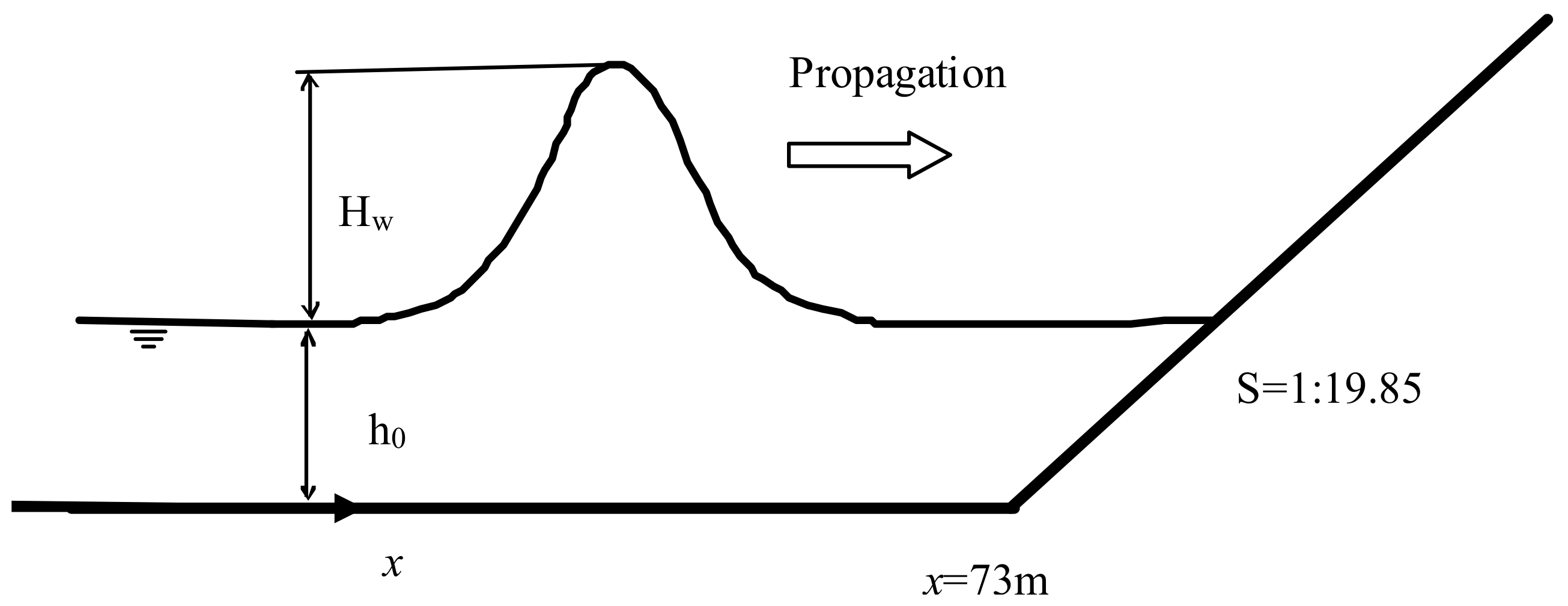
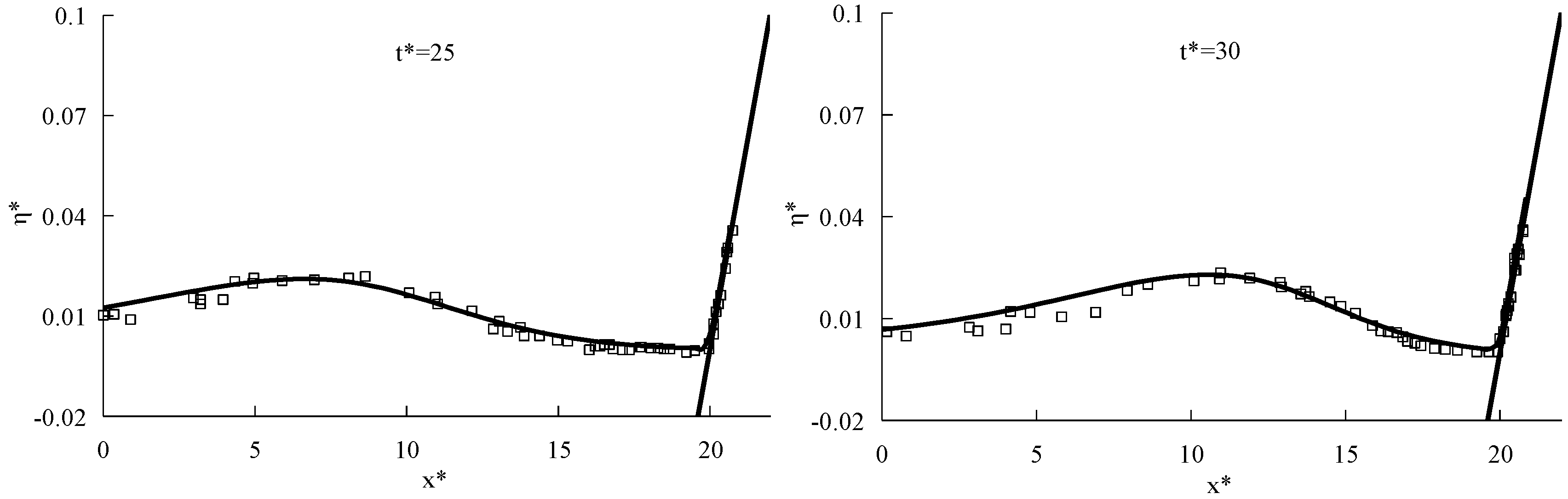
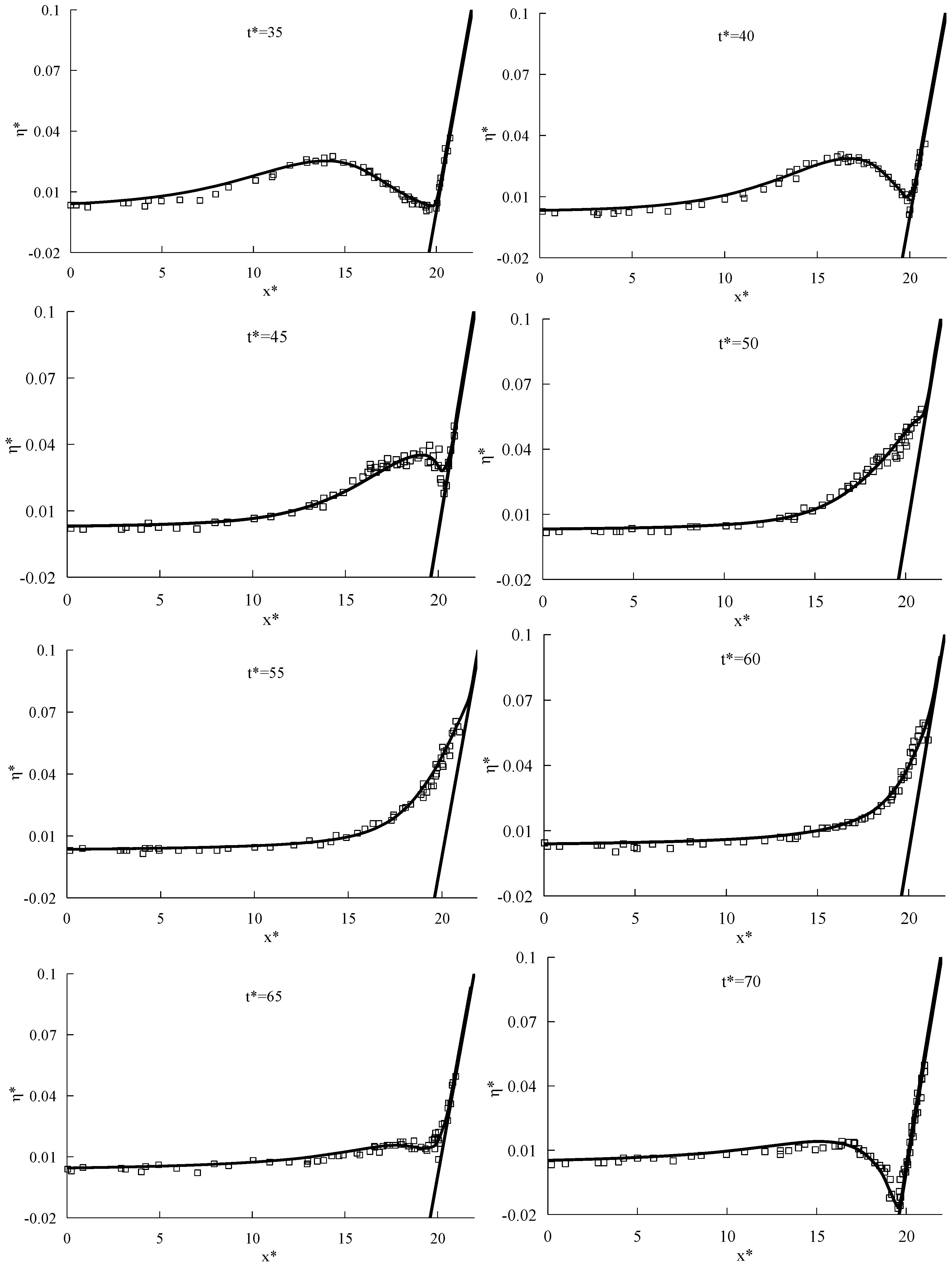
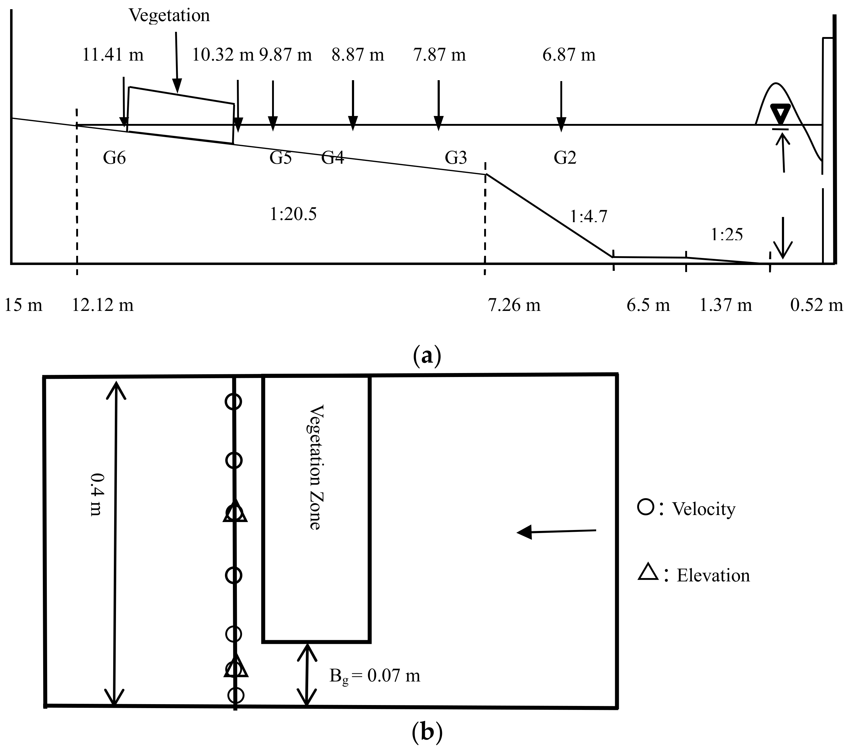
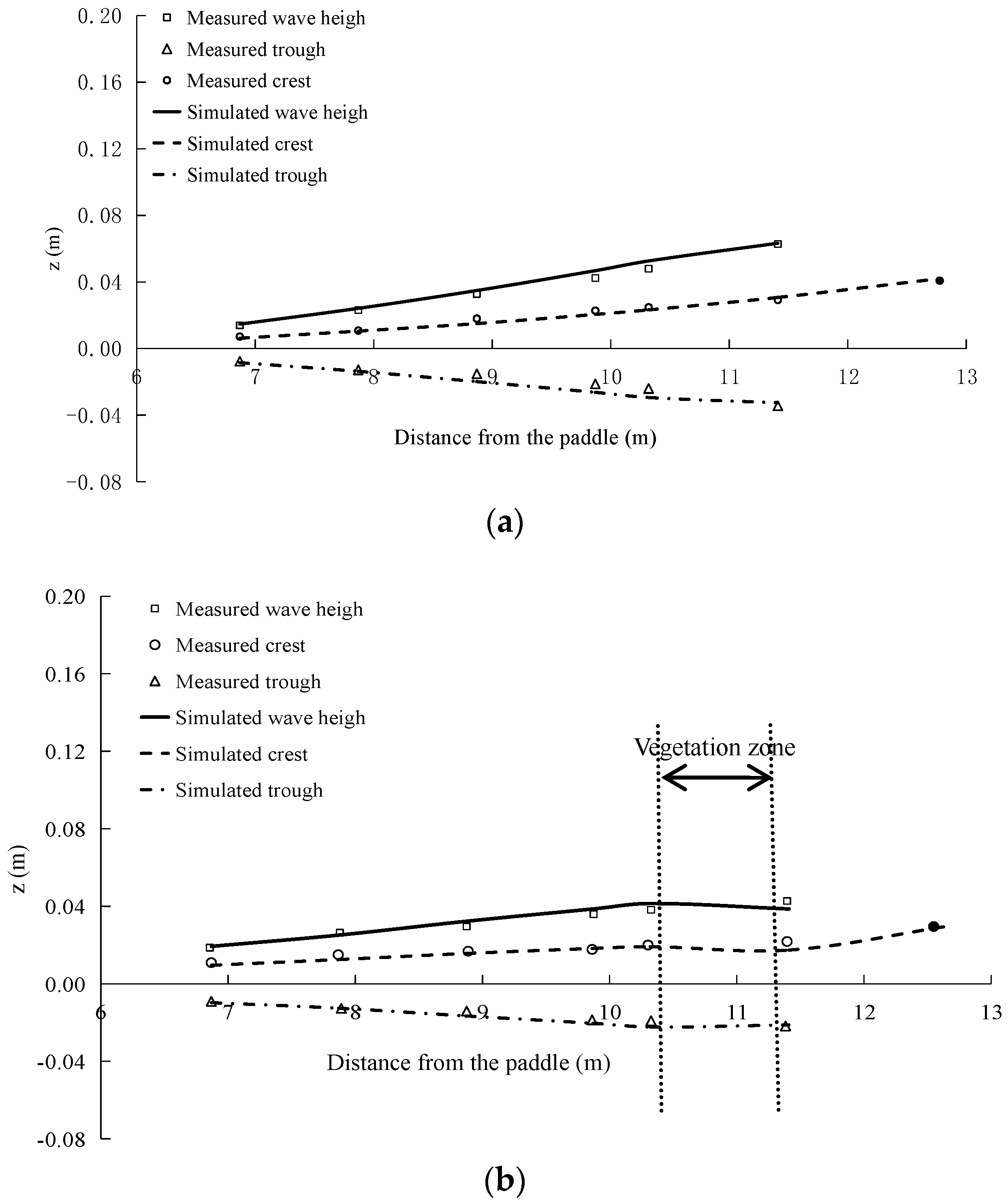
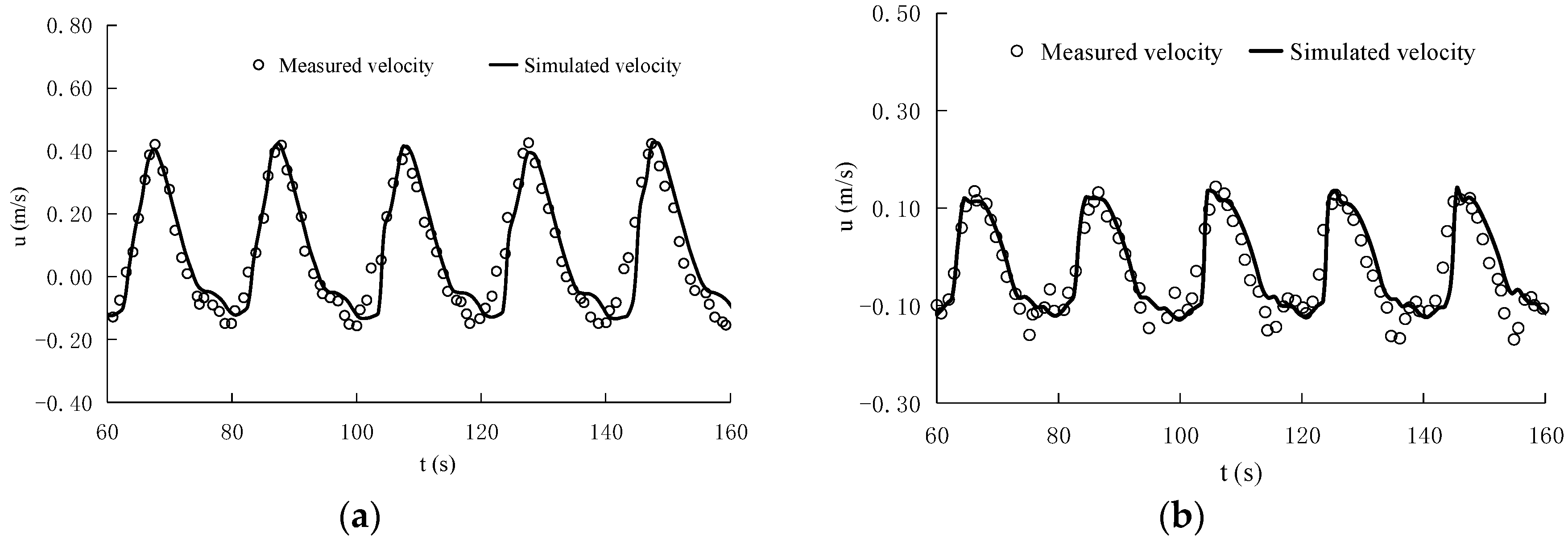
3.2. Propagation of Long Periodic Waves on a Partially Vegetated Sloping Beach

A laboratory experiment exploring the propagation of long periodic waves in a wave channel with a partially-vegetated sloping beach was conducted in Saitama University [31,32]. In this experiment, the wave tank was 15 m long and 0.4 m wide for propagation, and the bed profile of the beach consisted of several sections with various slopes (Figure 5a). The vegetation was modelled using wooden cylinders with a diameter of 0.005 m at a still water depth of 0.44 m. The vegetation domain was from x = 10.36 to 11.36 m, with different vegetation gap widths (Bg = 0, 0.07, and 0.4 m), while the vegetation density was set as 2200 stem/m−2, and the drag coefficient CD of wooden cylinders was calibrated as 2.5 in the present study. An incident sinusoidal wave with a period of T = 20 s and wave height of 0.16 cm was propagated from a 0.52 m long constant bottom segment to a sloping beach. In the current case, water surface elevations were measured using capacitance wave gauges at six positions (G1–G6) along the center of the flume in cases of Bg = 0 and 0.4 m, and the flow velocities were measured using electromagnetic current meters at locations in the cross section passing behind vegetation domain G6 (see Figure 5b) in case of Bg = 0.07 m. The run-up height above still water surface was measured by tracing the moving of water front by eyes with a scale on the slope. The computational domain was represented by uniform triangular cells with a grid spacing of 0.01 m and a time step of 0.002 s for the numerical model. The minimum depth criterion for a dry and wet bed was considered as 0.001 m, and the Manning coefficient was set as 0.012.
A comparison of wave crests, heights, and troughs in Figure 6a,b demonstrates that for the case of non-vegetated areas, wave heights increased due to shoaling as the long waves approached shallow water, however, the increased amplitudes of wave heights were attenuated by the resistance effects of vegetation at the sloping zone, with the attenuated rate reaching 38.96% at G6 (at the center behind vegetation). The wave height at the front of the vegetated zone was also affected by the reflection of waves caused by the vegetation. Figure 7 shows the comparison of time series of velocities at the center of the gap exit and the center of the end of the vegetation when Bg = 0.07 m, indicating that the peak flow velocity at the center of the gap exit can reach 0.42 m/s and is 3.07 times more than the peak flow velocity at behind the center of the vegetation zone. Figure 8 shows the distribution of the peak velocities averaged from five wave periods at steady state in a cross-section of Gage 6, indicating that vegetation plays an important role in the distribution of flow velocities. The results demonstrate that the present model is an effective tool to predict long periodic wave propagation on a partially vegetated sloping beach. Vegetation can effectively attenuate the wave propagation; however, an open gap in vegetation zone generates large flow and adverse effect at gap exit.

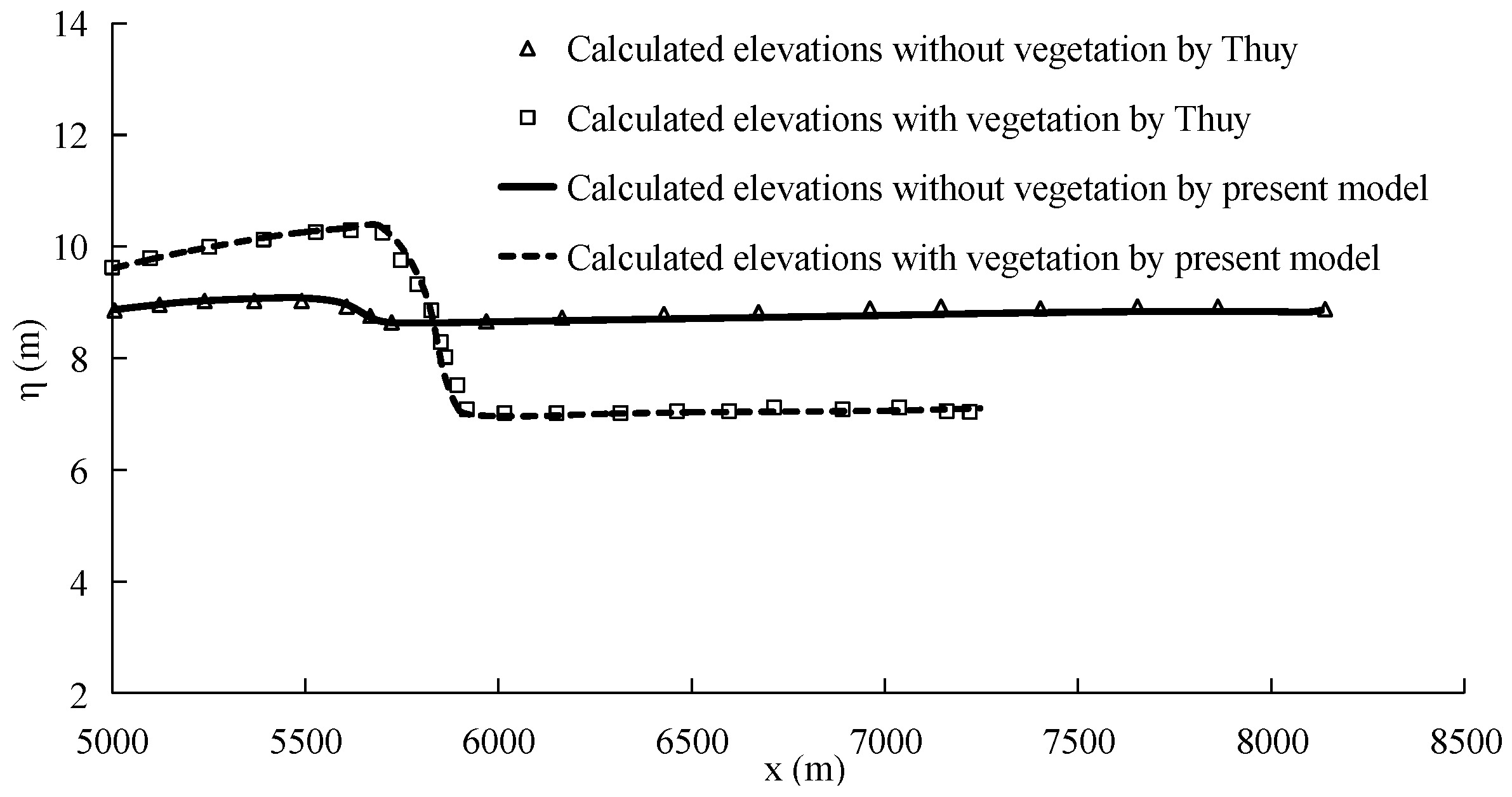
3.3. Effects of Forest on Tsunami Run-up at Actual Scale

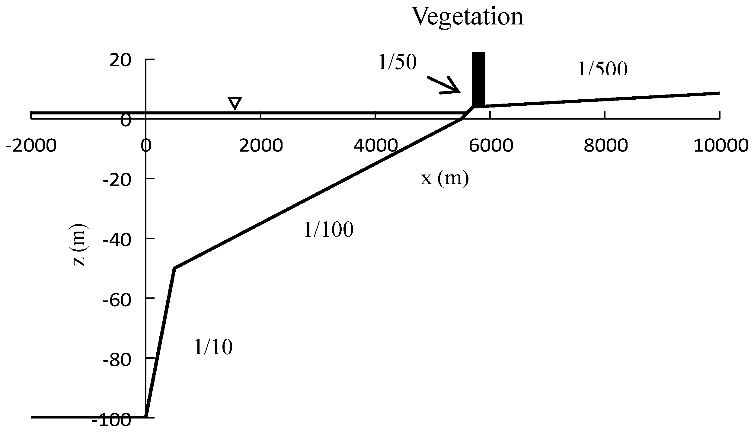
3.3.1. Coastal Topography and Forest Conditions

Coastal forests are widely considered to mitigate tsunami damage on coastal beaches in some countries and regions. In this case study, a numerical simulation was performed to investigate the run-up of tsunami and the effects of forest vegetation on tsunami mitigation. A coastal topography adopted for tsunami simulation is presented in Figure 9 [25,31]. The bed profile of the computed domain consisted of four slopes: S = 1/10, 1/100, 1/50, and 1/500, while the offshore water depth with a horizontal bed was 102 m below the still water level, all parameters for a tsunami wave simulation can be seen in references [25,31].
P. odoratissimus is a representative tree of South and Southeast Asia with a complex aerial root structure growing in coastal beach. In addition, C. equisetifolia is another representative species that grows densely on sandy beaches. These two species are discussed in evaluating the resistance of vegetation on tsunami propagation. The tree heights hv of P. odoratissimus and C. equisetifolia are considered as 8 m and 11 m, respectively; the reference diameters bref of P. odoratissimus and C. equisetifolia are set as 0.2 m and 0.15 m, respectively; and the density values N of P. odoratissimus and C. equisetifolia are 0.22 trees/m2 and 0.4 trees/m2, respectively. The depth-averaged equivalent drag coefficient CD(h) are variable with vegetation parameters and inundation depth h, and they are modified by Tanaka et al. and Thuy et al. [22,26]. The coastal forest starts at a slope of 1/500 (see Figure 9).
In this numerical simulation, the computational domain is discretized into 38,010 triangular meshes, in which the coarsest grid spacing at the sea-side is 20 m, and the finest grid spacing is 2.5 m at the nearshore area. The Manning’s roughness coefficient is set as 0.02 for the computational domain. By comparing the maximum water surface elevations in Figure 10, there is good agreement between the simulated and Thuy’s results [31].
In non-vegetated areas, as the wave crest approaches a 1/50 slope, its energy compresses and the maximum water surface elevations increase slightly because of shoaling. When the wave crest approaches a slope of 1/500, the maximum water surface elevations decrease due to the accelerated flow velocity on a mild slope. For fully vegetated areas, the maximum water surface elevations increase significantly at the front of the forest due to the reflection of the waves caused by the vegetation. In the forest zone, the maximum water surface elevations decrease drastically. The run-up height above the still water level is 5.10 m with full vegetation, which is lower than the 6.86 m for non-vegetation areas. The results indicate that P. odoratissimus effectively protects coastal communities from the destruction by a tsunami wave by reducing wave energy.

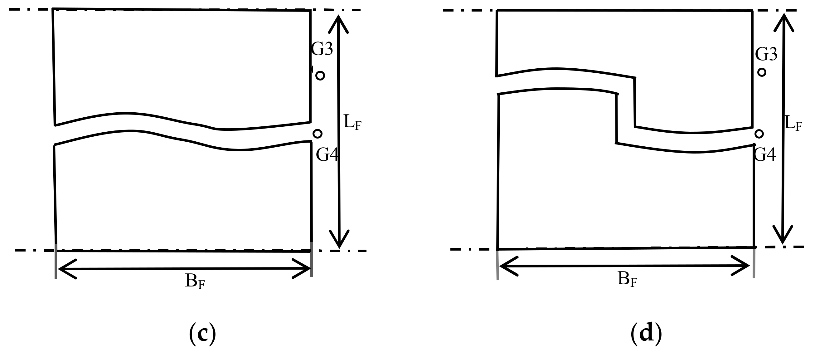
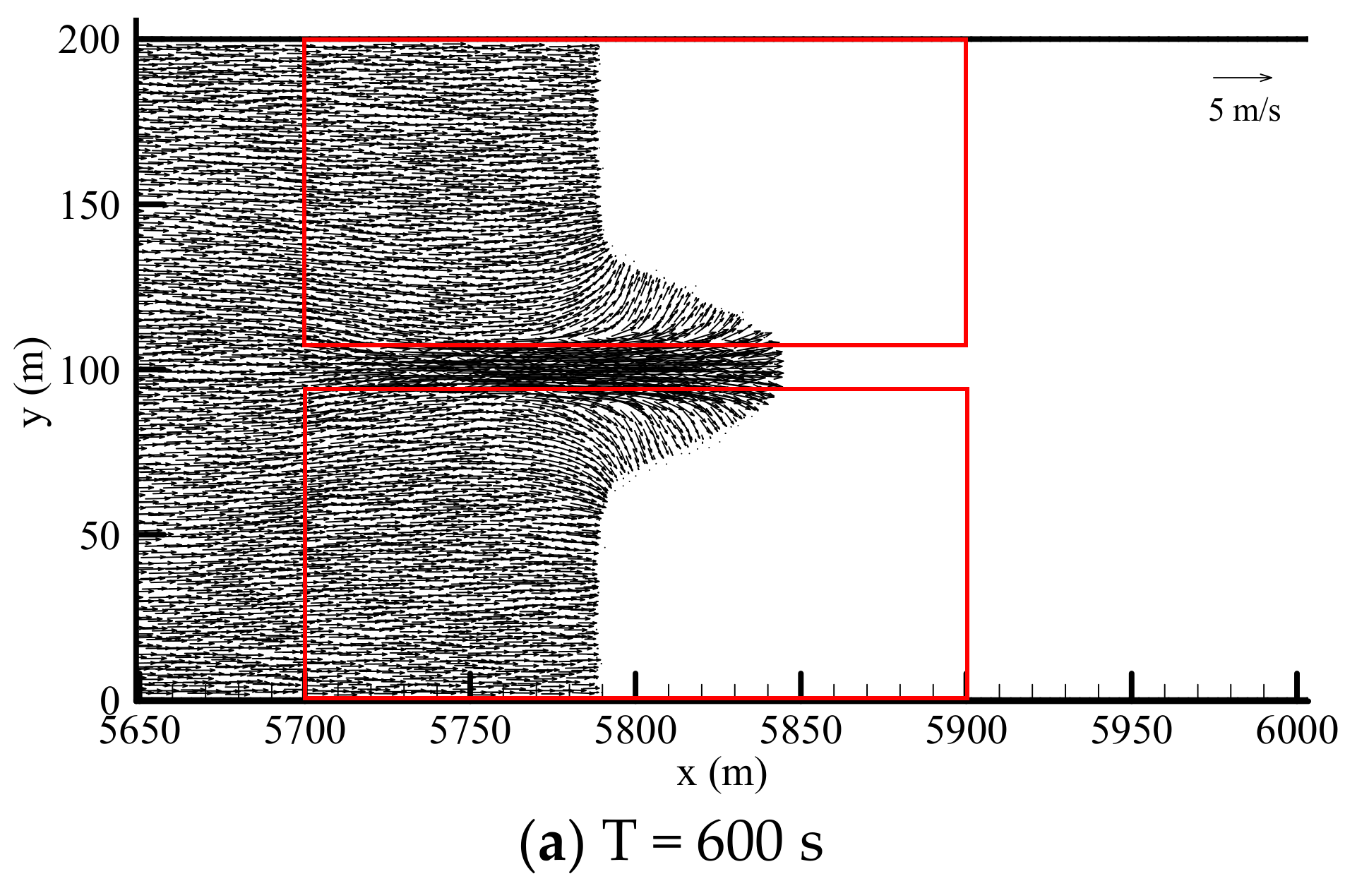
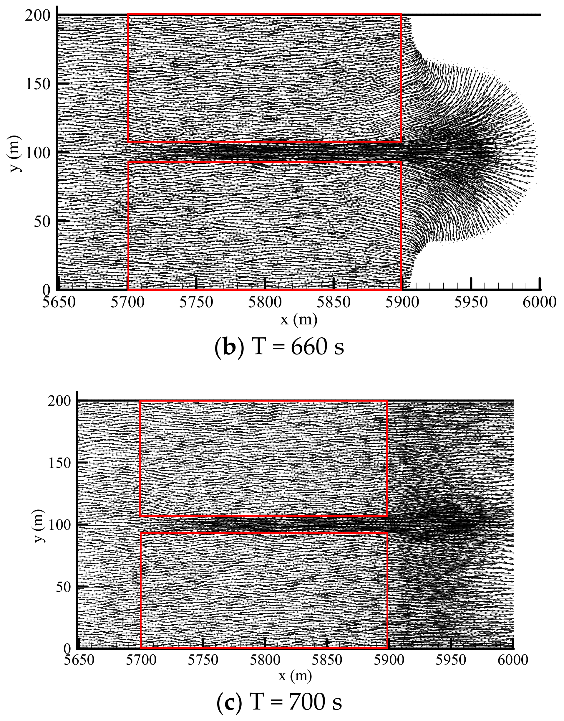
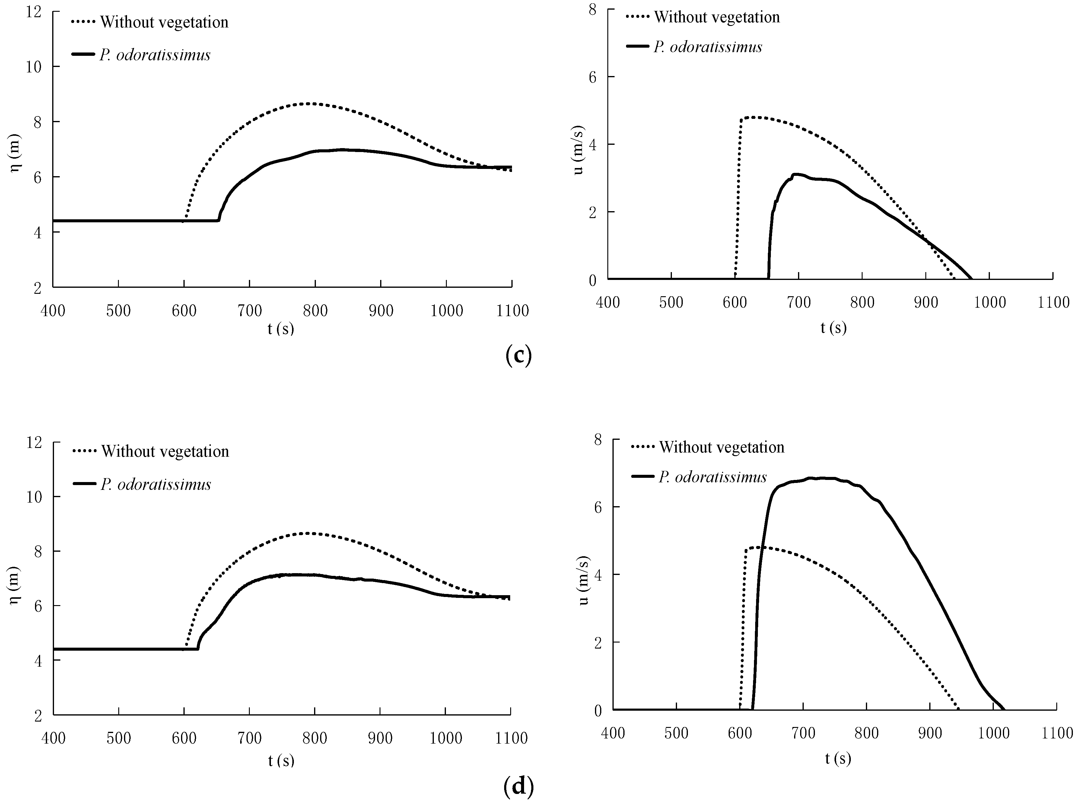
3.3.2. Effects of Forest with a Straight Open Gap on Tsunami Run-up

Figure 11 shows four types of gap arrangements (Cases 1, 2, 3, and 4) in P. odoratissimus forest with the simulation conditions of LF = 200 m, BF = 200 m, and BG = 15 m. In this section, tsunami run-up on the sloping beach is considered using a straight gap (Case 1) to investigate the effect on tsunami run-up.
Figure 12a–c presents the predicted flow structure in Case 1 at different times (600, 660 and 700 s). The flow velocity of the first wave is fast in an open gap zone, while the wave moves slowly in the forest domain due to the resistance from vegetation. The first wave front quickly passes the open gap and spreads out from the exit, and the flow behind the forest gradually becomes uniform, with the exception of the areas close to the gap exit. Figure 13 shows the temporal variation of water surface elevations and flow velocities at four predicted stations (G1, G2, G3, and G4) for Case 1. In this case, the maximum water surface elevations in the presence of vegetation are higher at G1 (the middle of the open gap) and G2 (the middle before the vegetation) than those in the absence of vegetation due the reflection of tsunami waves caused by P. odoratissimus forest.
As the flow passes the forest, the maximum water surface elevations drastically decrease. The maximum water surface elevation values at G3 (the middle behind the forest) and G4 (the middle at the end of the open gap) in the presence of vegetation with an open gap decrease to 80.72% and 82.52% of that for the case of non-vegetation, respectively. The time delays in a tsunami arriving at G3 and G4 are about 45 and 14 s, respectively, when the wave passes through forest with an open gap compared to that of non-vegetated case. The P. odoratissimus forests slightly impact the peak velocities at G1 and G2, which reach 4.36 and 4.35 m/s, respectively. Due the resistance effects of P. odoratissimus, the flow velocities at G1 and G2 decrease dramatically after reaching their peak. The peak velocity at G3 is decreased by 35.13% and the peak velocity at G4 is increased by 44.04%. The open gap in forest vegetation amplifies negative effects on tsunami propagation even more than in the non-vegetated case.

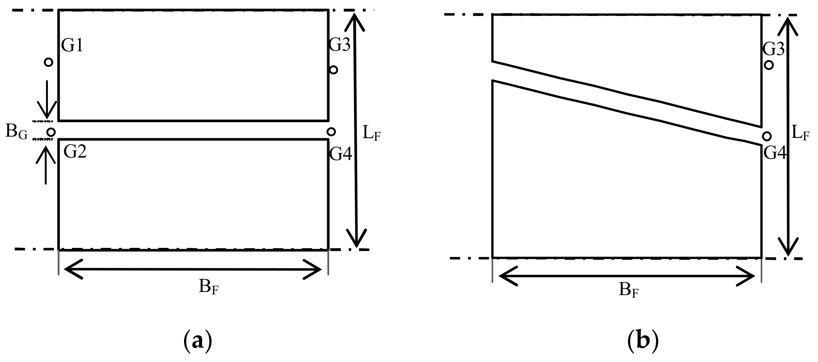
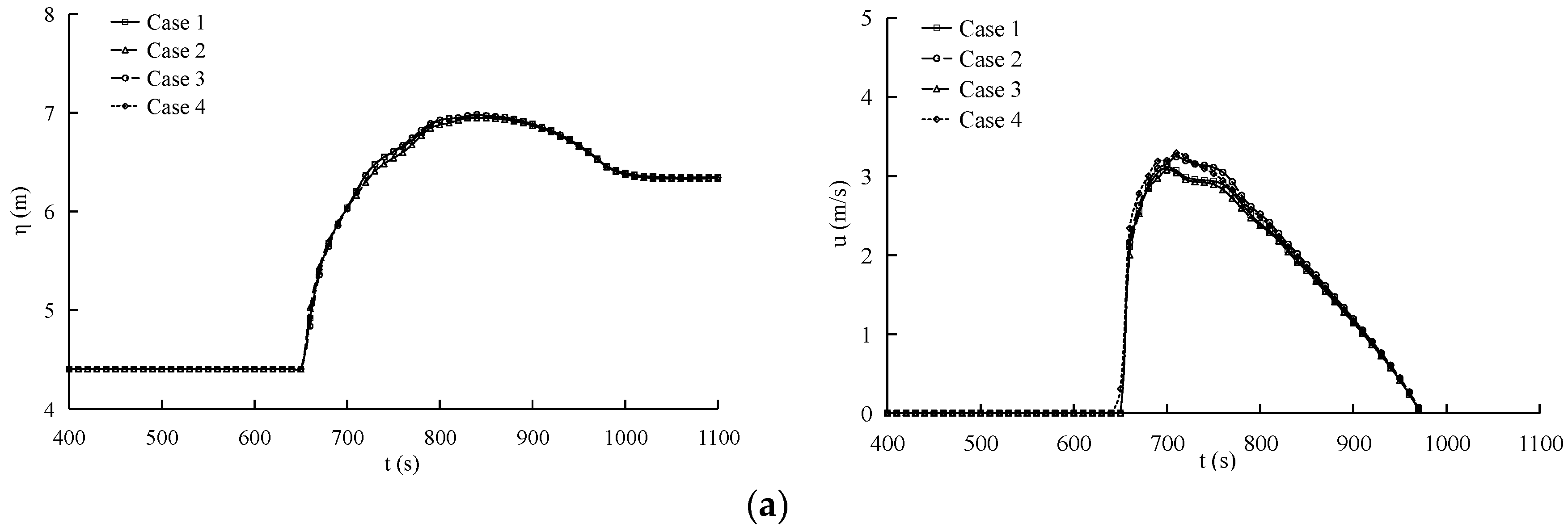
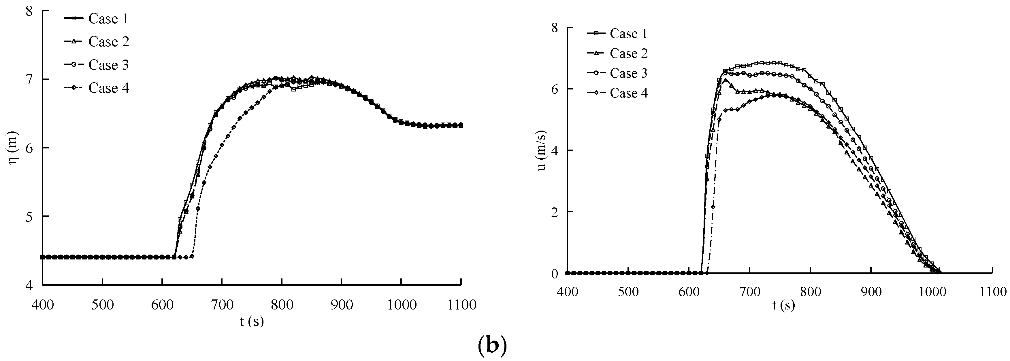
3.3.3. Effects of Arrangements of Vegetation Patches and Open Gaps

Four types of gap structures are discussed to investigate their potential to increase the energy attenuation of tsunami waves on a vegetated beach. Figure 14 illustrates the structures of a flow field at 660 s for three cases with different gap arrangements, and shows that the flow velocities are larger in open gaps than those in vegetated zones, and the front of the first wave quickly passes the open gap, and the maximum peak flow velocities appear around the gap exit. The furthest distance that tsunami waves reach is variable, but there are differences in flow where structures occur. As presented in Figure 15, the effects of the gap arrangements on the water surface elevations at G3 and G4 are insignificant for four cases, while the different gap arrangements have important effects on flow velocities of tsunami waves.
Compared to Case 1, the peak flow velocities at the G3 station are increased by about 0.15 m/s (4.92%) and 0.21 m/s (6.71%) for Case 2 and Case 4, respectively, and the peak flow velocity is attenuated slightly by about 0.05 m/s (−1.46%) for Case 3. Compared to Case 1, the peak flow velocities at G4 are decreased by about 0.47 m/s (−6.77%), 0.34 m/s (−4.87%) and 0.89 m/s (−12.88%) for Case 2, 3, and 4, respectively. Figure 16 shows the comparisons of the run-up heights of the first tsunami wave for different cases including fully vegetated, non-vegetated, and four types of vegetation arrangements with different gaps. The results indicate that the slight differences of run-up heights occur for different gap arrangements, however, the presence of vegetation significantly attenuates the energy of tsunami waves compared to non-vegetated case. Therefore, it is reasonable to reduce the disadvantages from open gaps by changing gap arrangements.

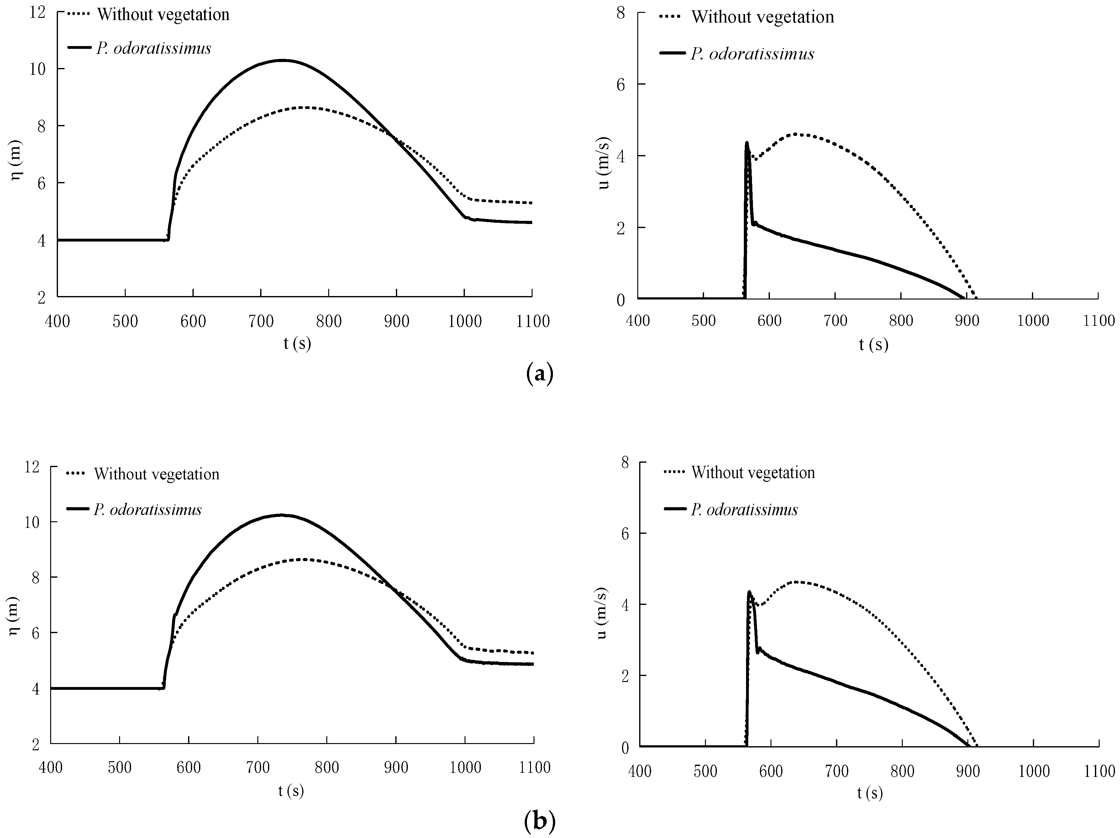
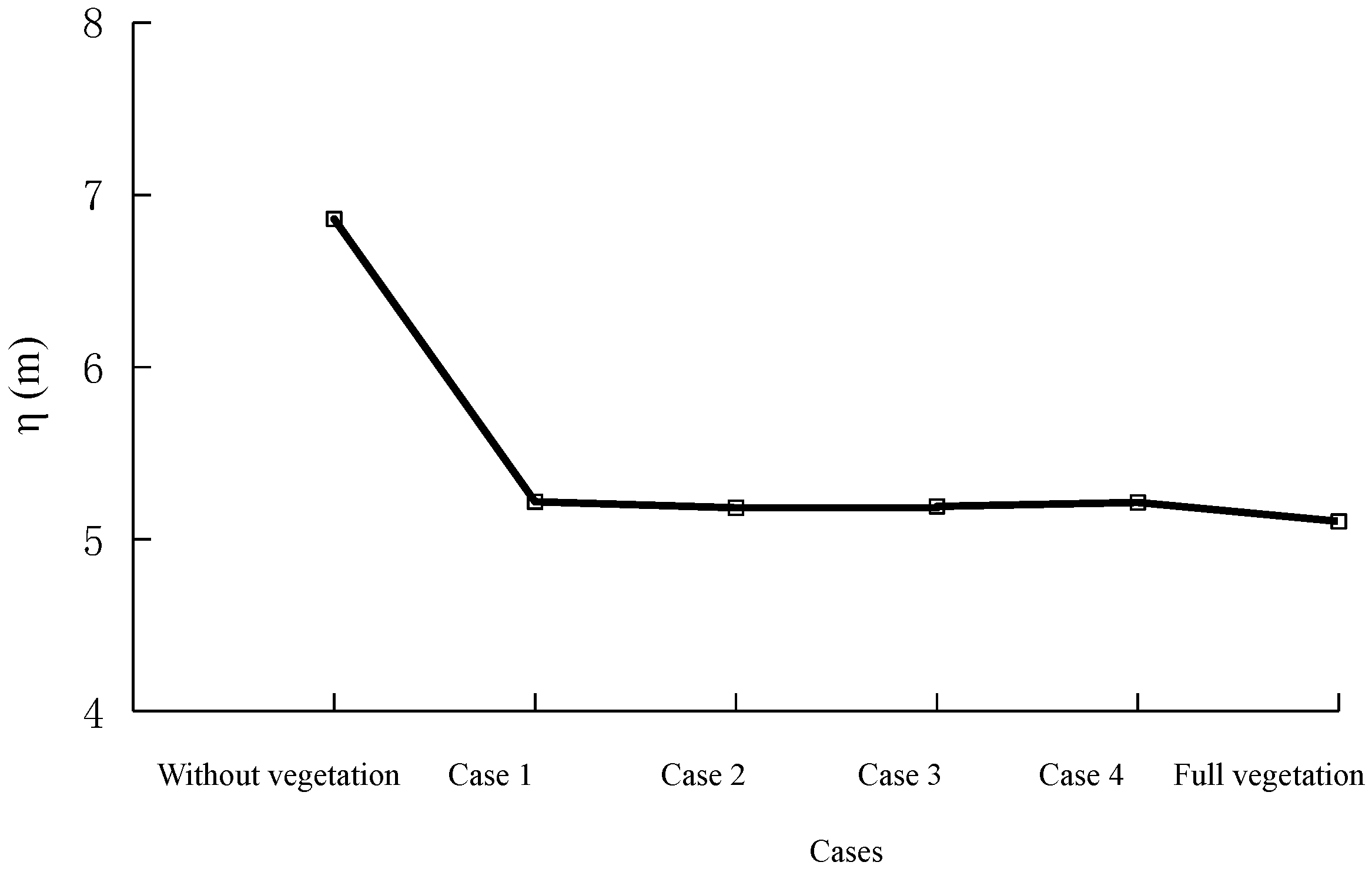
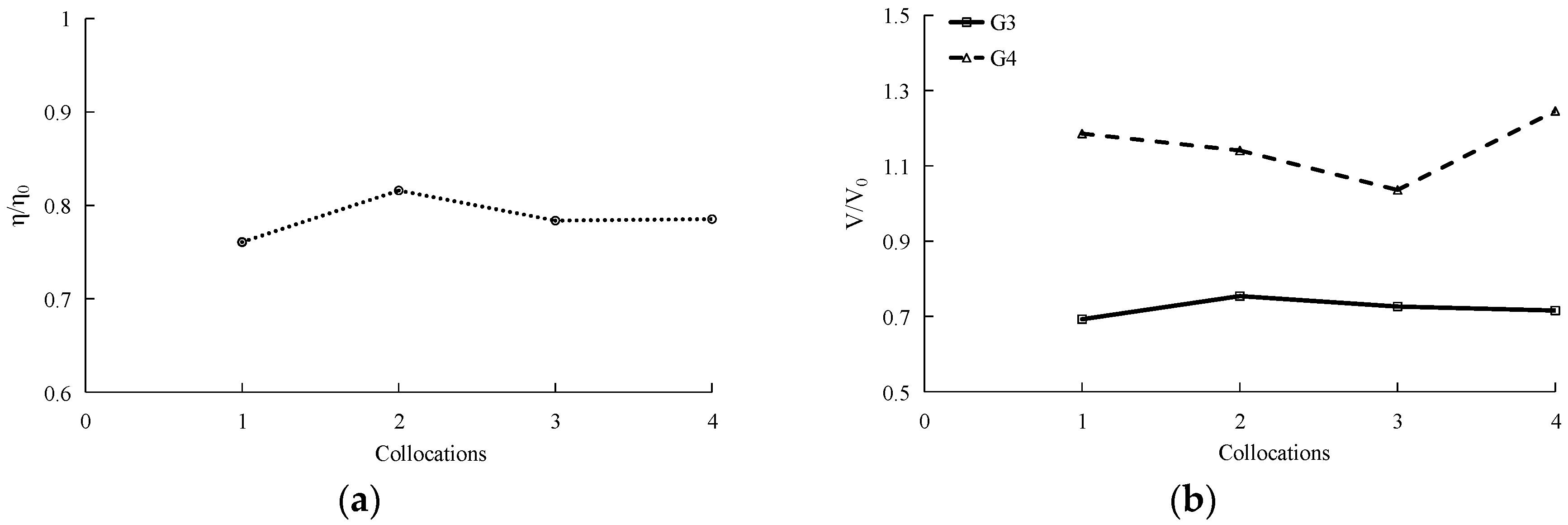
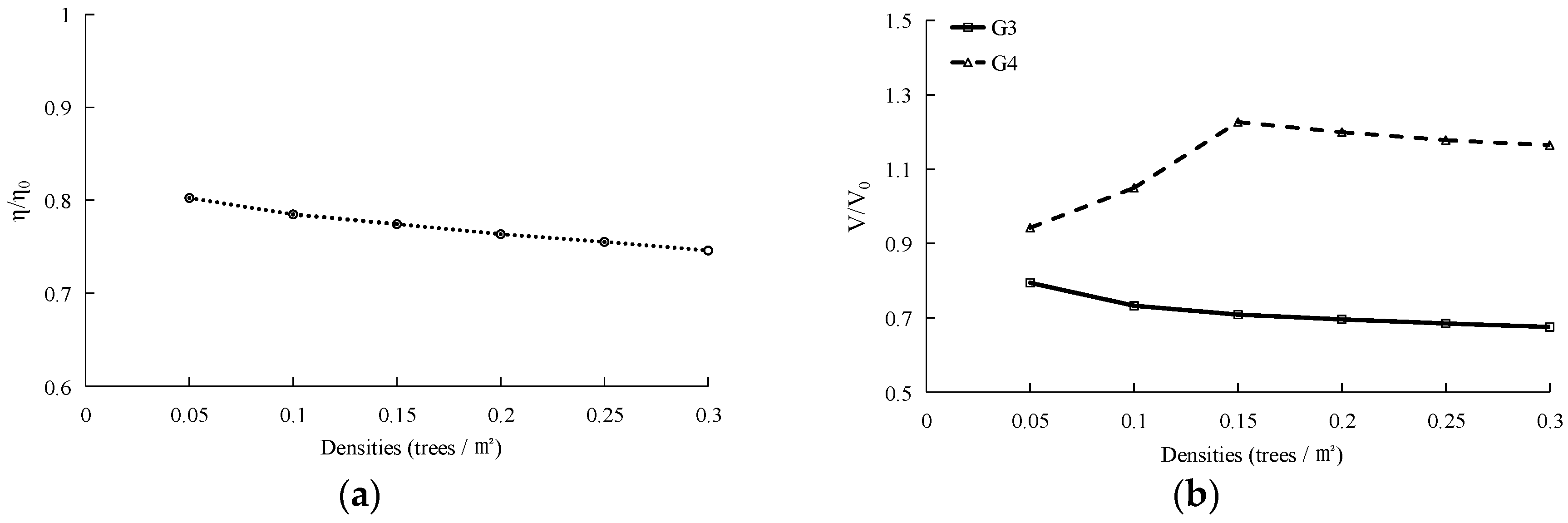
3.3.4. Effects of Forest Parameters on Tsunami Run-up

To investigate the effects of coastal forest parameters on tsunami run-up, a sensitivity analysis of different tree configurations, densities, and growth stages was examined in the gap arrangement of Case 4. In this section, Collocation 1 (pure P. odoratissimus), Collocation 2 (pure C. equisetifolia), Collocation 3 (C. equisetifolia as the back vegetation layer of P. odoratissimus), and Collocation 4 (C. equisetifolia as the front vegetation layer of P. odoratissimus) are considered to analyze effects of tree configuration on tsunami propagation. Figure 17 shows the variation of normalized run-up heights (η/η0) and normalized peak flow velocities (V/V0) at simulated gauges (G3 and G4) with different tree arrangements, respectively, where η0 and V0 denote the run-up height and the peak flow velocity in the absence of vegetation. The results indicate that C. equisetifolia as a new vegetation layer at the back of existing P. odoratissimus (Collocation 3) can minimize the amplification of the peak flow velocity through the open gap, while generating a slightly larger peak flow velocity at the G3 station. The run-up height is higher than that of Collocation 1 (pure P. odoratissimus) and smaller than that of Collocation 2. This is because the peak flow velocity is reduced significantly due greater resistance of P. odoratissimus when it passes the P. odoratissimus vegetation layer, and in back zone of C. equisetifolia vegetation with smaller drag force, the velocity increment in open gap is smaller compared to that of other tree configurations.In Collocation 1 (pure P. odoratissimus), Figure 18 indicates that normalized run-up height and normalized peak flow velocity at G3 decreased monotonously with increased densities, while the normalized peak flow velocity of G4 first increased (vegetation density ≤ 0.15 tree/m2) and then presented adverse variation. Figure 19 indicates that the increased vegetation height and diameter at different growth stages of P. odoratissimus generate positively correlated effects on normalized peak flow velocity at G4, and significant attenuation effects on normalized run-up height and normalized peak flow velocity at G3. Generally, changing forest parameters (e.g. vegetation collocations, densities and growth stages) could be a more cost-effective way to mitigate tsunami damage.

4. Conclusions

Based on the shallow water equations of mass and momentum, an explicit depth-averaged 2D numerical model was developed to simulate wave attenuation and tsunami wave mitigation in a vegetated coastal region. The finite volume method was used to keep conservation of mass in this model. The proposed model was well verified for both breaking and non-breaking solitary wave propagations on a bare sloping beach, and long periodic wave propagation on a partially-vegetated sloping beach, as shown by comparison of experimental data. Overall, the present numerical model has been shown to accurately account for wave propagation and transformation in vegetated and non-vegetated sloping beaches.
In the case of full P. odoratissimus forest on an actual-scale beach, the water surface elevations at the front of the forest belt increased due to the effect of reflected waves caused by vegetation. Here, P. odoratissimus forest played a positive role in reducing maximum water surface elevations through the vegetated zone, and as such the maximum wave run-up height of the tsunami was effectively reduced. When a forest has an open gap, the negative effects can be reduced by choosing a beneficial arrangement of vegetation and open gaps. Sensitivity analysis was also carried out by changing tree collocation, tree densities, and growth stage, with results showing that they had important impacts in reducing the peak flow velocity of the tsunami wave at the open gap exit.
Overall, these study findings provide cost-effective natural strategies to improve the effectiveness of P. odoratissimus forests with an open gap by changing vegetation arrangements and vegetation parameters (collocations, tree densities, and growth stage), which are important in the design and establishment of vegetated bioshields against tsunami hazards.

Author Contributions

H.Z. contributed to the establishment of model, significantly to analysis and manuscript preparation. M.Z. contributed to the conception of the study and the final editing. T.X. and J.T. contributed to the collection of experimental data.

Funding

This work was supported by the National Nature Science Foundation of China (51779039, 51879028), the Wetland Degradation and Ecological Restoration Program of Panjin Pink Beach (PHL-XZ-2017013-002), the Fund of Liaoning Marine Fishery Department (201725).

Conflicts of Interest

The authors declare no conflict of interest.

References

  1. Gopinath, G.; Løvholt, F.; Kaiser, G.; Harbitz, C.B.; Srinivasa, R.K.; Ramalingam, M.; Singh, B. Impact of the 2004 Indian ocean tsunami along the Tamil Nadu coastline: field survey review and numerical simulations. Nat. Hazards 2014, 72, 743–769. [Google Scholar] [CrossRef]
  2. Gelfenbaum, G.; Apotsos, A.; Stevens, A.W.; Jaffe, B. Effects of fringing reefs on tsunami inundation American Samoa. Earth Sci. Rev. 2011, 107, 12–22. [Google Scholar] [CrossRef]
  3. Liu, H.; Shimozono, T.; Takagawa, T.; Okayasu, A.; Fritz, H.; Sato, S.; Tajima, Y. The 11 March 2011 Tohoku tsunami survey in rikuzentakata and comparison with historical event. Pure Appl. Geophys. 2013, 170, 1033–1046. [Google Scholar] [CrossRef]
  4. Sarfaraz, M.; Pak, A. SPH numerical simulation of tsunami wave forces impinged on bridge superstructures. Coast. Eng. 2017, 121, 145–157. [Google Scholar] [CrossRef]
  5. Touhami, H.E.; Khellaf, M.C. Laboratory study on effects of submerged obstacles on tsunami wave and run-up. Nat. Hazards 2017, 87, 757–771. [Google Scholar] [CrossRef]
  6. Hsiao, S.C.; Lin, T.C. Tsunami-like solitary waves impinging and overtopping an impermeable seawall: experiment and RANS modeling. Coast. Eng. 2010, 57, 1–18. [Google Scholar] [CrossRef]
  7. Irish, J.L.; Weiss, R.; Yang, Y.; Yang, Y.; Song, Y.; Zainali, A.; Marivela-Colmenarejo, R. Laboratory experiments of tsunami run-up and withdrawal in patchy coastal forest on a steep beach. Nat. Hazards 2014, 74, 1933–1949. [Google Scholar] [CrossRef]
  8. Ko, H.T.S.; Yeh, H. On the splash-up of tsunami bore impact. Coast. Eng. 2018, 131, 1–11. [Google Scholar] [CrossRef]
  9. Witt, D.L.; Yin, L.Y.; Yim, S.C. Field investigation of tsunami impact on coral reefs and coastal sandy slopes. Mar. Geol. 2011, 289, 159–163. [Google Scholar] [CrossRef]
  10. Fritz, H.M.; Petroff, C.M.; Catalán, P.A.; Cienfuegos, R.; Winckler, P.; Kalligeris, N.; Weiss, R.; Barrientos, S.E.; Meneses, G.; Valderas-Bermejo, C.; et al. Field Survey of the 27 February 2010 Chile Tsunami. Pure Appl. Geophys. 2011, 168, 1989–2010. [Google Scholar] [CrossRef]
  11. Shuto, N. Numerical simulation of tsunamis-Its present and near future. Nat. Hazards 1991, 4, 171–191. [Google Scholar] [CrossRef]
  12. Li, L.; Qiu, Q.; Huang, Z. Numerical modeling of the morphological change in Lhok Nga, west banda aceh, during the 2004 Indian ocean tsunami: Understanding tsunami deposits using a forward modeling method. Nat. Hazards 2012, 64, 1549–1574. [Google Scholar] [CrossRef]
  13. Suppasri, A.; Imamura, F.; Koshimura, S. Effects of the rupture velocity of fault motion, ocean current and initial sea level on the transoceanic propagation of tsunami. Coast. Eng. J. 2010, 52, 107–132. [Google Scholar] [CrossRef]
  14. Ryan, K.J.; Geist, E.L.; Barall, M.; Oglesby, D.D. Dynamic models of an earthquake and tsunami offshore Ventura, California. Geophys. Res. Lett. 2015, 42, 6599–6606. [Google Scholar] [CrossRef] [Green Version]
  15. Maris, F.; Kitikidou, K. Tsunami hazard assessment in Greece-Review of numerical modeling (numerical simulations) from twelve different studies. Renew. Sust. Energ. Rev. 2016, 59, 1563–1569. [Google Scholar] [CrossRef]
  16. Qu, K.; Ren, X.; Kraatz, S. Numerical investigation of tsunami-like wave hydrodynamic characterics and its comparison with solitary wave. Appl. Ocean Res. 2017, 63, 36–48. [Google Scholar] [CrossRef]
  17. Kerr, A.M.; Baird, H.B. Natural barriers to natural disasters. Bioscience 2017, 57, 102–103. [Google Scholar] [CrossRef]
  18. Okal, E.; Fritz, H.M.; Synolakis, C.E.; Borrero, J.C. Field survey of the Samoa tsunami of 29 September. Seismol. Res. Lett. 2010, 81, 577–591. [Google Scholar] [CrossRef]
  19. Augustin, L.N.; Irish, J.L.; Lynett, P. Laboratory and numerical studies of wave damping by emergent and near-emergent wetland vegetation. Coast. Eng. 2009, 5, 332–340. [Google Scholar] [CrossRef]
  20. Yang, Z.; Tang, J.; Shen, Y. Numerical study for vegetation effects on coastal wave propagation by using nonlinear Boussinesq model. Appl. Ocean Res. 2018, 70, 32–40. [Google Scholar] [CrossRef]
  21. Tanaka, N.; Ogino, K. Comparison of reduction of tsunami fluid force and additional force due to impact and accumulation after collision of tsunami-produced driftwood from a coastal forest with houses during the Great East Japan tsunami. Landscape Ecol. Eng. 2017, 13, 287–304. [Google Scholar] [CrossRef]
  22. Feagin, R.A.; Mukherjee, N.; Shanker, S.; Baird, A.H.; Cinner, J.; Kerr, A.M.; Koedam, N.; Sridhar, A.; Arthur, R.; Jayatissa, L.P.; et al. Shelter from the storm? Use and misuse of coastal vegetation bioshields for managing natural disasters. Conserv. Lett. 2010, 3, 1–11. [Google Scholar] [CrossRef] [Green Version]
  23. Bayas, J.C.L.; Marohn, C.; Dercon, G.; Dewi, S.; Piepho, H.P.; Joshi, L.; Noordwijk, M.V.; Cadisch, G. Influence of coastal vegetation on the 2004 tsunami wave impact in west Aceh. Proc. Natl. Acad. Sci. USA 2011, 108, 18612–18617. [Google Scholar] [CrossRef] [PubMed] [Green Version]
  24. Tanaka, N.; Nandasena, N.A.K.; Jinadasa, K.S.B.N.; Sasaki, Y.; Tanimoto, K.; Mowjood, M.I.M. Developing effective vegetation bioshield for tsunami protection. J. Civ. Environ. Eng. Syst. 2009, 26, 163–180. [Google Scholar] [CrossRef]
  25. Thuy, N.B.; Tanaka, N.; Tanimoto, K. Tsunami mitigation by coastal vegetation considering the effect of tree breaking. J. Coast. Conserv. 2012, 16, 111–121. [Google Scholar] [CrossRef]
  26. Iimura, K.; Tanaka, N. Numerical simulation estimating effects of tree density distribution in coastal forest on tsunami mitigation. Ocean Eng. 2012, 54, 223–232. [Google Scholar] [CrossRef]
  27. Yang, Y.Q.; Irish, J.L.; Weiss, R. Impact of patchy vegetation on tsunami dynamics. Waterw. Port Coastal Ocean Eng. 2017, 143, 04017005. [Google Scholar] [CrossRef]
  28. Tanaka, N.; Yasuda, S.; Iimura, K.; Yagisawa, J. Combined effects of coastal forest and sea embankment on reducing the washout region of houses in the Great East Japan tsunami. J. Hydro-Environ. Res. 2014, 8, 270–280. [Google Scholar] [CrossRef]
  29. Mascarenhas, A.; Jayakumar, S. An environmental perspective of the post-tsunami scenario along the coast of Tamil Nadu, India: Role of sand dunes and forests. J. Environ. Manag. 2008, 89, 24–34. [Google Scholar] [CrossRef]
  30. Tanimoto, K.; Tanaka, N.; Thuy, N.B.; Nandasena, N.A.K.; Iimura, K. Effect of open gap in coastal forest on tsunami run-up—investigation by 2-dimensional numerical simulation. Ocean Eng. 2008, 24, 87–92. (In Japanese) [Google Scholar]
  31. Thuy, N.B.; Tanimoto, K.; Tanaka, N.; Harada, K.; Iimura, K. Effect of open gap in coastal forest on tsunami run-up-investigations by experiment and numerical simulation. Ocean Eng. 2009, 36, 1258–1269. [Google Scholar] [CrossRef]
  32. Nandasena, N.A.K.; Sasaki, Y.; Tanaka, N. Modeling field observations of the 2011 Great East Japan tsunami: Efficacy of artificial and natural structures on tsunami mitigation. Coast. Eng. 2012, 67, 1–13. [Google Scholar] [CrossRef]
  33. Zhang, M.; Li, C.; Shen, Y. Depth-averaged modeling of free surface flow in open channels with emerged and submerged vegetation. Appl. Math. Model. 2013, 37, 540–553. [Google Scholar] [CrossRef]
  34. Liang, Q.; Borthwick, A.G.L. Adaptive quadtree simulation of shallow flows with wet-dry fronts over complex topography. Comput. Fluids 2009, 38, 221–234. [Google Scholar] [CrossRef]
  35. Brufau, P.; García-Navarro, P.; Vázquez-Cendón, M.E. Zero mass error using unsteady wetting-drying conditions in shallow flows over dry irregular topography. Int. J. Numer. Methods Fluids 2004, 45, 1047–1082. [Google Scholar] [CrossRef]
  36. Synolakis, C.E. The run-up of long waves. Ph D Thesis, California Institute of Technology, Pasadena, CA, USA, January 1986. [Google Scholar]
  37. Wu, W.; Marsooli, R. A depth-averaged 2D shallow water model for breaking and non-breaking long waves affected by rigid vegetation. J. Hydraul. Res. 2012, 50, 558–575. [Google Scholar] [CrossRef]
  38. Tang, J.; Causon, D.; Mingham, C.; Qian, L. Numerical study of vegetation damping effects on solitary wave run-up using the nonlinear shallow water equations. Coast. Eng. 2013, 75, 21–28. [Google Scholar] [CrossRef]
Figure 1. Schematic diagram of wet-dry edges.
Water 10 01776 g001
Figure 2. Sketch of the solitary wave propagation on a sloping beach.
Water 10 01776 g002
Figure 3. Run-up and run-down of Hw/h0 = 0.0185 non-breaking solitary wave on a 1:19.85 sloping beach.
Water 10 01776 g003aWater 10 01776 g003b
Figure 4. Run-up and run-down of Hw/h0 = 0.3 breaking solitary wave on a 1:19.85 sloping beach.
Water 10 01776 g004aWater 10 01776 g004b
Figure 5. Experimental setup of wave flume. (a) Longitudinal section, (b) plan view of vegetation zone and measurement points.
Water 10 01776 g005
Figure 6. Comparison of measured and calculated wave crests, heights, and troughs. (a) Case without vegetation, (b) Case with full vegetation.
Water 10 01776 g006
Figure 7. Time series of velocities, (a) at the center of the gap exit, (b) at the center of the end of the vegetation.
Water 10 01776 g007
Figure 8. Transverse profiles of maximum velocity in a cross-section of Gage 6 (Bg = 0.07 m).
Water 10 01776 g008
Figure 9. Schematic topography of a tsunami flume with vegetation effects.
Water 10 01776 g009
Figure 10. Maximum water surface elevations of the first wave without vegetation and with P. odoratissimus vegetation [26].
Water 10 01776 g010
Figure 11. Sketch of gap arrangements, (a) Case 1, (b) Case 2, (c) Case 3, (d) Case 4.
Water 10 01776 g011aWater 10 01776 g011b
Figure 12. Flow structure in Case 1 at different times ((a) T = 600 s, (b) T = 660 s, (c) T = 700 s).
Water 10 01776 g012aWater 10 01776 g012b
Figure 13. Temporal variation of water surface elevations and flow velocities at four predicted stations of Case 1, (a) G1, (b) G2, (c) G3, (d) G4.
Water 10 01776 g013aWater 10 01776 g013b
Figure 14. Flow structures at 660 s: (a) Case 2, (b) Case 3, and (c) Case 4.
Water 10 01776 g014
Figure 15. Temporal variation of surface water elevations and current velocities at (a) = G3 and (b) = G4.
Water 10 01776 g015aWater 10 01776 g015b
Figure 16. The comparison of maximum run-up heights.
Water 10 01776 g016
Figure 17. Variation of normalized run-up heights and normalized peak flow velocities at G3 and G4 with different tree collocations, (a) The normalized run-up heights, (b) The normalized peak flow velocities.
Water 10 01776 g017
Figure 18. Variation of normalized run-up heights and normalized peak flow velocities at G3 and G4 with different densities of pure P. odoratissimus. (a) The normalized run-up heights, (b) The normalized peak flow velocities.
Water 10 01776 g018
Figure 19. Variation of normalized run-up heights and normalized peak flow velocities at G3 and G4 with different heights of pure P. odoratissimus; (a) The normalized run-up heights, (b) The normalized peak flow velocities.
Water 10 01776 g019

