Accounting for the Spatio-Temporal Variability of Pollutant Processes in Stormwater TSS Modeling Based on Stochastic Approaches


Abstract
1. Introduction
2. Materials and Methods
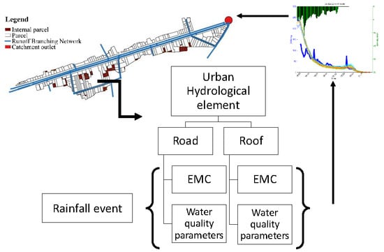
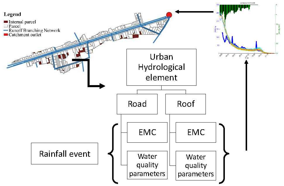
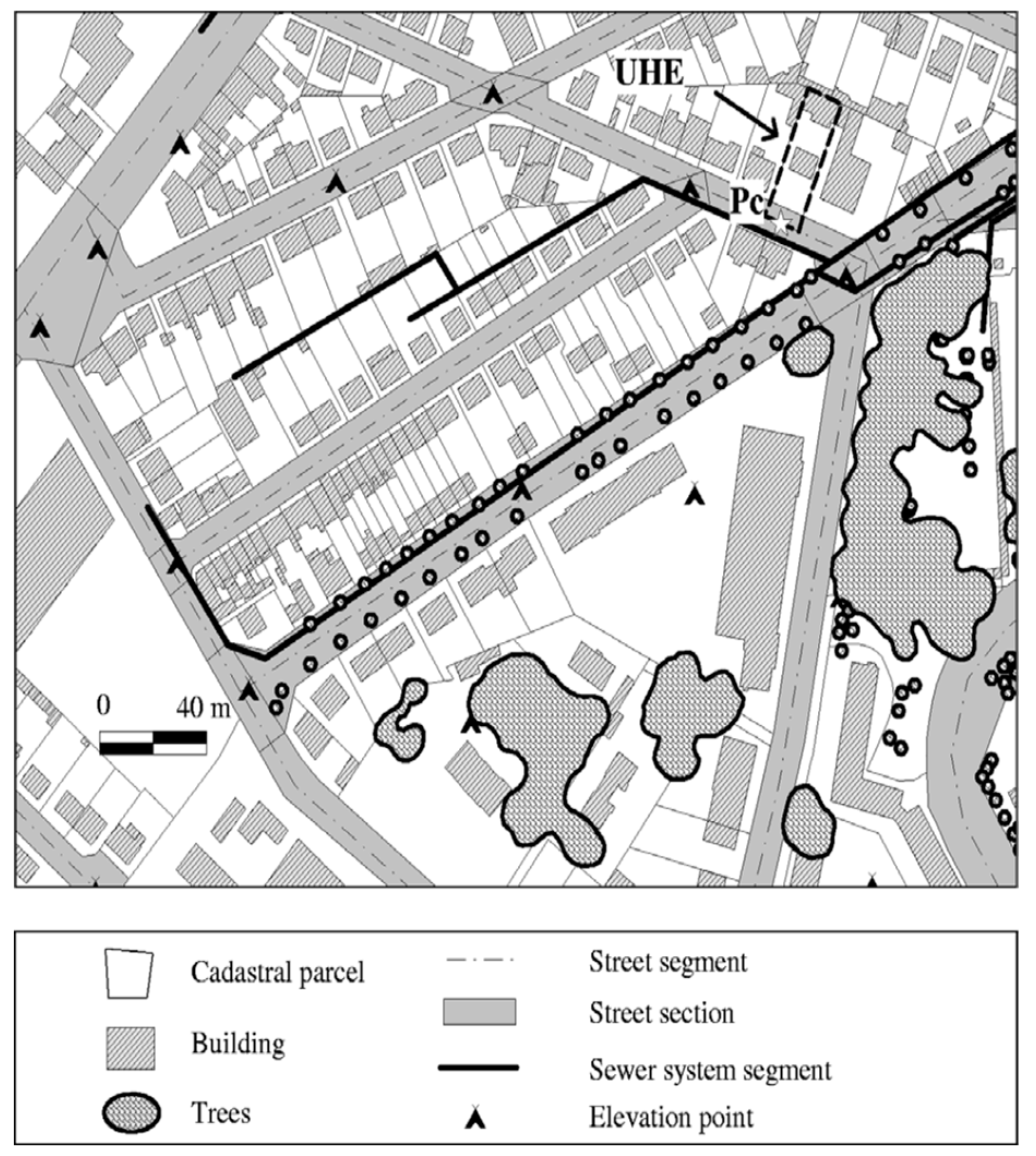
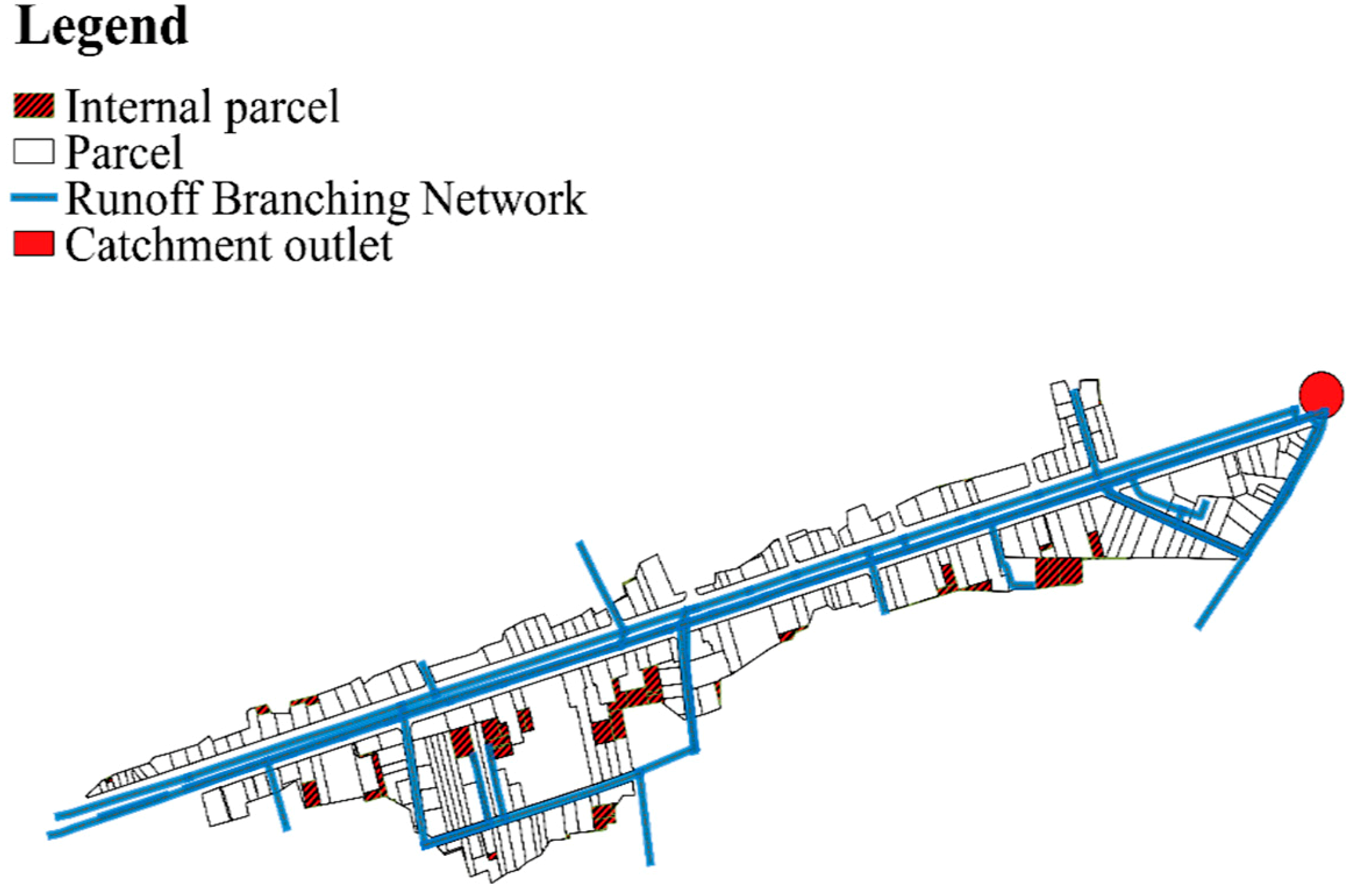
2.1. Hydrological Model URBS
Model Implementation
2.2. Stormwater Quality Modeling
2.2.1. Stochastic Approach
2.2.2. The Models
2.2.3. Boundaries of the Sampling Ranges
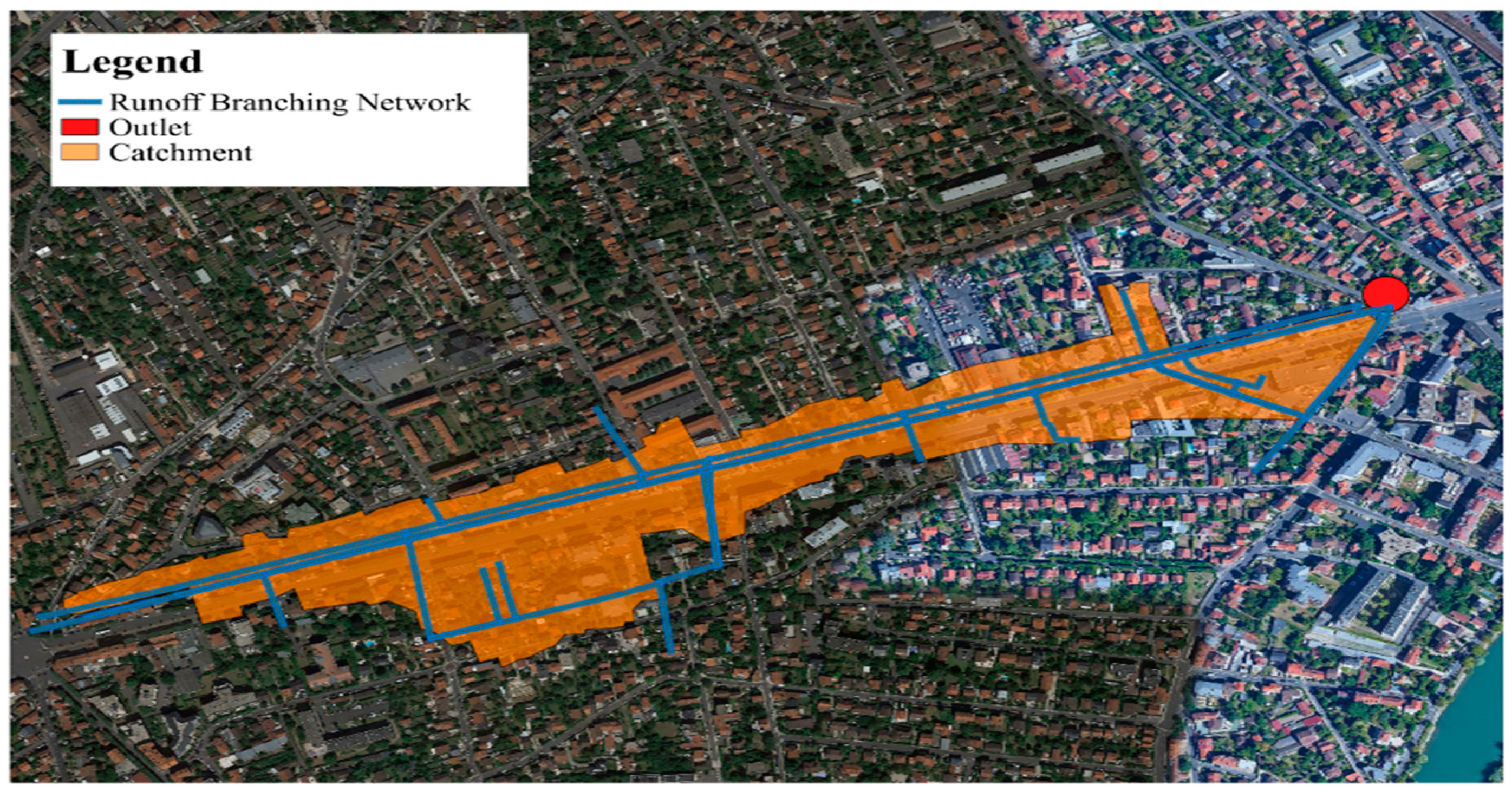
2.3. Catchment and Data Description
2.4. Evaluation Criterion of the Model Performance
2.5. Model Application
3. Results and Discussion
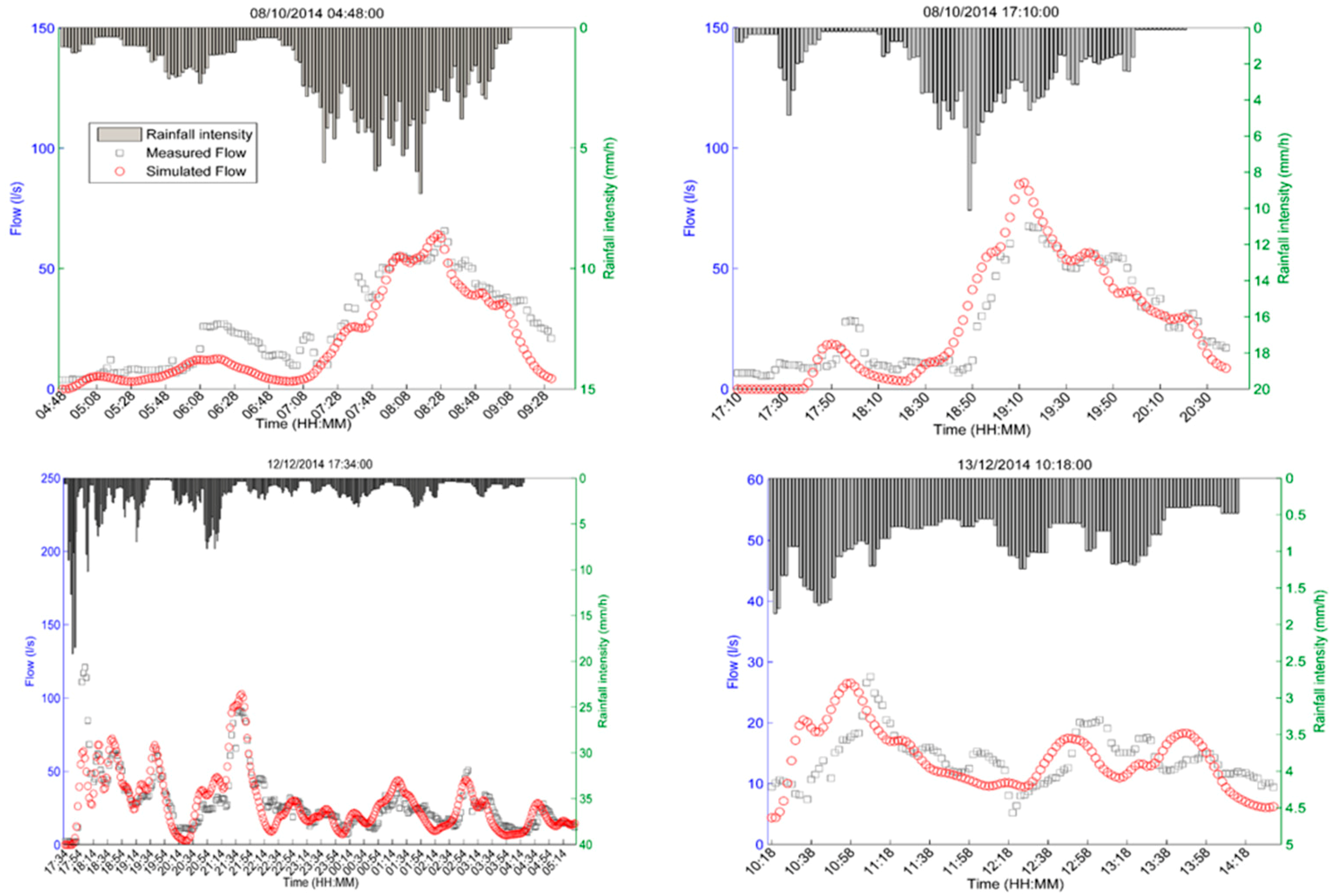
3.1. Water Flow Simulations
3.2. Water Quality Modeling
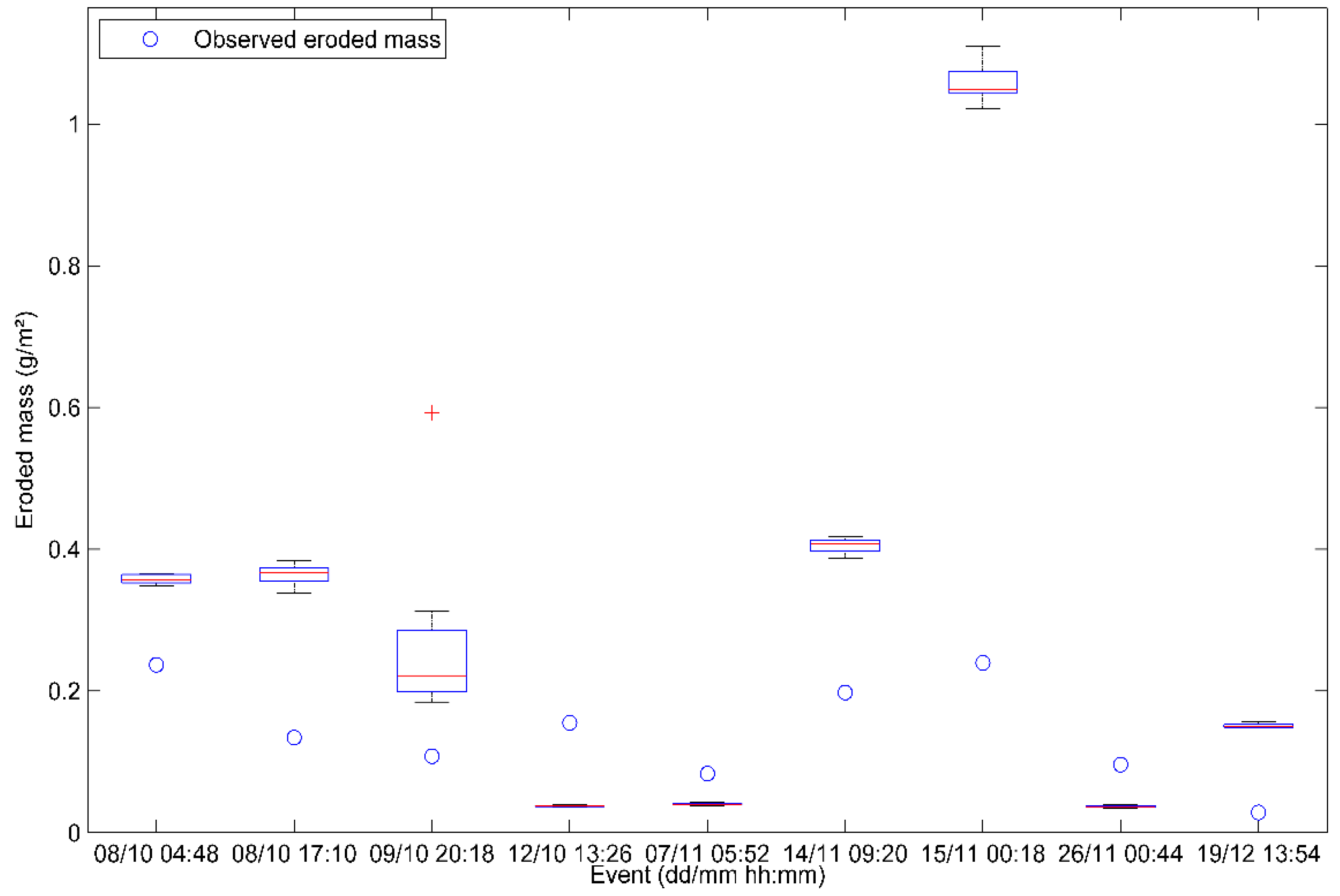
3.2.1. TSS Loads
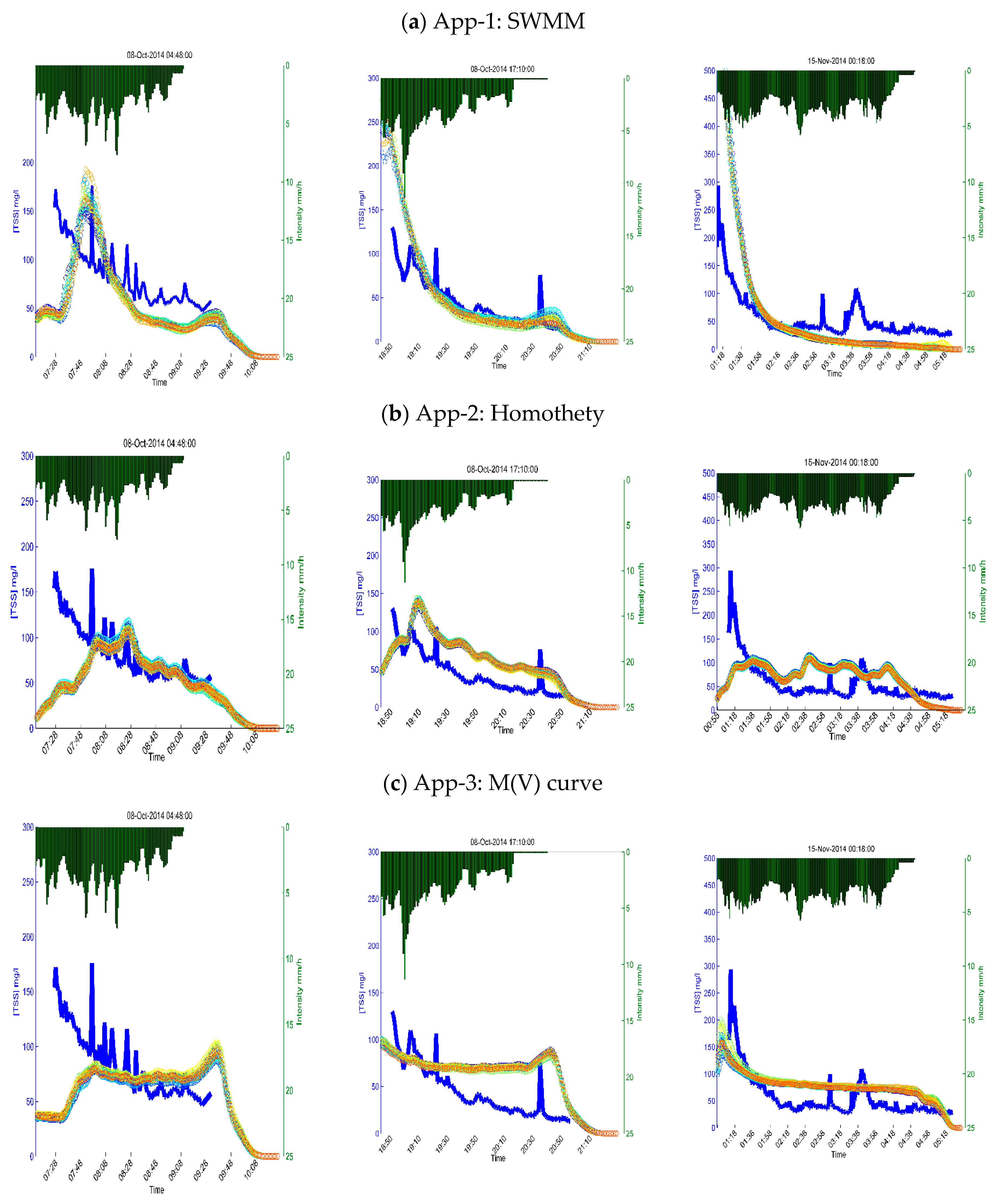
3.2.2. TSS Dynamics
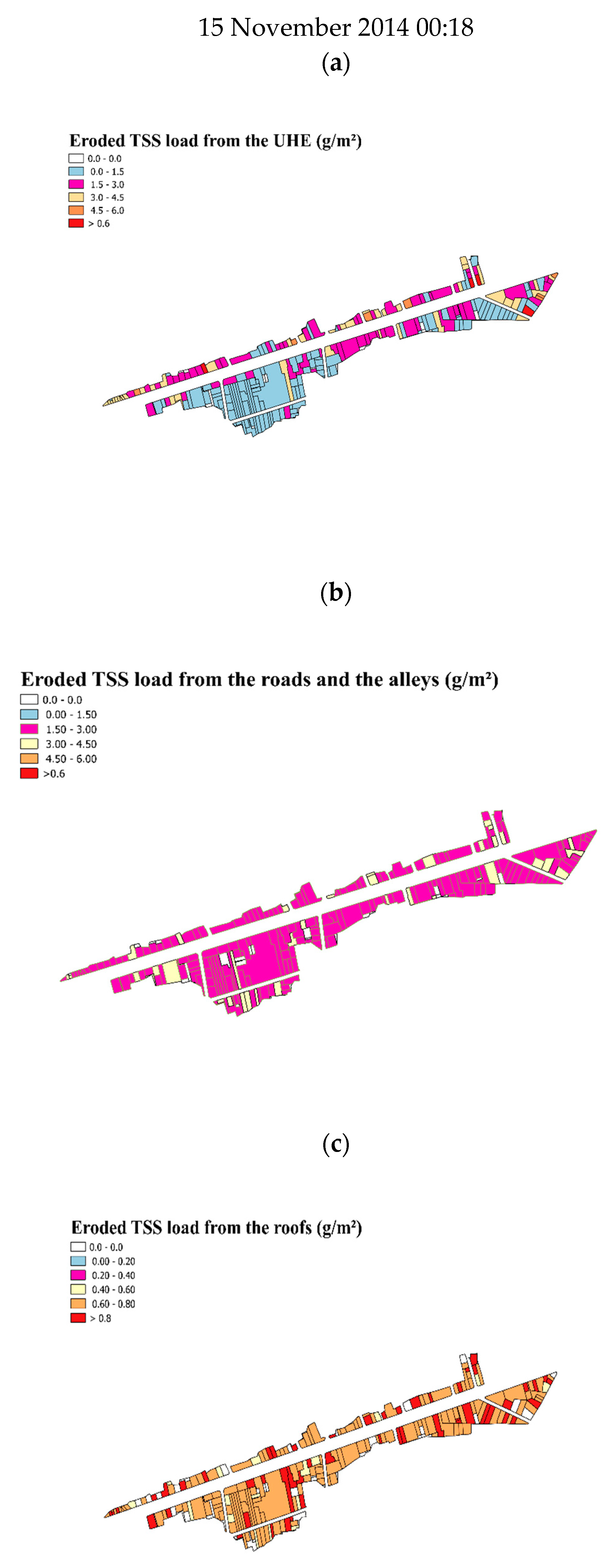
3.2.3. Spatial Variability of TSS Loads
4. Conclusions
Author Contributions
Funding
Conflicts of Interest
Appendix A

| Duration (min) | ADWP (hours) | Rainfall Depth (mm) | Maximum Intensity (mm/h) | |
|---|---|---|---|---|
| Min | 52 | 0.8 | 2 | 1.1 |
| Max | 720 | 274.4 | 22.1 | 42.3 |
| Mean | 185.4 | 61.7 | 5.7 | 8.3 |
| Median | 124 | 37.2 | 3.8 | 5.3 |
| d10 | 57.6 | 1.7 | 2.3 | 1.1 |
| d90 | 347 | 175.1 | 11.9 | 15.2 |
| Beginning Date | End Date | Duration (min) | ADWP (hours) | Precipitation Height (mm) | Maximum Intensity (mm/h) |
|---|---|---|---|---|---|
| 8 Oct. 2014 04:48 | 8 Oct. 2014 09:34 | 288 | 11.8 | 9.1 | 6.89 |
| 8 Oct. 2014 17:10 | 8 Oct. 2014 20:40 | 212 | 8 | 7.47 | 10.1 |
| 9 Oct. 2014 20:18 | 9 Oct. 2014 21:10 | 54 | 24 | 4.63 | 42 |
| 12 Oct. 2014 13:26 | 12 Oct. 2014 15:22 | 118 | 64.5 | 3.54 | 6.9 |
| 7 Nov. 2014 05:52 | 7 Nov. 2014 07:54 | 124 | 76.5 | 3.77 | 6.71 |
| 14 Nov. 2014 09:20 | 14 Nov. 2014 13:08 | 230 | 170 | 7.42 | 7.95 |
| 15 Nov. 2014 00:18 | 15 Nov. 2014 04:42 | 266 | 11.4 | 12.83 | 5.54 |
| 26 Nov. 2014 00:44 | 26 Nov. 2014 02:34 | 112 | 221 | 3.4 | 4.99 |
| 19 Dec. 2014 13:54 | 19 Dec. 2014 16:04 | 132 | 52.7 | 3.39 | 12.2 |
| Parameter | Unit | Description | Value |
|---|---|---|---|
| Stree,min | mm | Minimum value of the tree interception | 1 |
| A | min−1 | Drainage law coefficient for tree interception | 0.04 |
| Smax,soil | Mm | Maximum capacity of the surface reservoir for the natural soil | 5 |
| Smax,roof | Mm | Maximum capacity of the surface reservoir for the roof | 0.5 |
| Smax,street | Mm | Maximum capacity of the surface reservoir for the street | 3.5 |
| Ks,soil | m/s | Hydraulic conductivity at natural saturation for the natural soil | 10−5 |
| Ks,street | m/s | Hydraulic conductivity at natural saturation for the street | 10−8 |
| M | - | Scaling parameter of the hydraulic conductivity | 5 |
| - | Water content at natural saturation | 0.43 | |
| - | Suction head at air entry | 0.05 | |
| Zroot | m | Root depth | 1.5 |
| Λ | - | Ground water drainage coefficient | 4 |
| µ | - | Ground water drainage exponent | 4 |
| αv | - | Representative position of the vadose zone | 0.5 |
| B | - | Retention curve exponent | 5 |
| X | Routing parameter of Muskingum | 0.2 | |
| Pipe filling rate | 2.51 |
References
- Lee, J.H.; Bang, K.W. Characterization of urban stormwater runoff. Water Res. 2000, 34, 1773–1780. [Google Scholar] [CrossRef]
- Kim, J.-Y.; Sansalone, J.J. Event-based size distributions of particulate matter transported during urban rainfall-runoff events. Water Res. 2008, 42, 2756–2768. [Google Scholar] [CrossRef]
- Göbel, P.; Dierkes, C.; Coldewey, W.G. Storm water runoff concentration matrix for urban areas. J. Contam. Hydrol. 2007, 91, 26–42. [Google Scholar] [CrossRef]
- Elliott, A.; Trowsdale, S. A review of models for low impact urban stormwater drainage. Environ. Model. Softw. 2007, 22, 394–405. [Google Scholar] [CrossRef]
- Zoppou, C. Review of urban storm water models. Environ. Model. Softw. 2001, 16, 195–231. [Google Scholar] [CrossRef]
- Tsihrintzis, V.A.; Hamid, R. Modeling and management of urban stormwater runoff quality: A review. Water Resour. Manag. 1997, 11, 136–164. [Google Scholar] [CrossRef]
- Dotto, C.B.S.; Kleidorfer, M.; Deletic, A.; Rauch, W.; McCarthy, D.T.; Fletcher, T.D. Performance and sensitivity analysis of stormwater models using a Bayesian approach and long-term high resolution data. Environ. Model. Softw. 2011, 26, 1225–1239. [Google Scholar] [CrossRef]
- Rossman, L.A. Storm Water Management Model User’s Manual, Version 5.0; National Risk Management Research Laboratory, Office of Research and Development, US Environmental Protection Agency Cincinnati: Washington, DC, USA, 2010. [Google Scholar]
- Bujon, G. Prévision des débits et des flux polluants transités par les réseaux d’égouts par temps de pluie. Le modèle FLUPOL. Houille Blanche 1988. [Google Scholar] [CrossRef]
- Sage, J.; Bonhomme, C.; Al Ali, S.; Gromaire, M.-C. Performance assessment of a commonly used “accumulation and wash-off” model from long-term continuous road runoff turbidity measurements. Water Res. 2015, 78, 47–59. [Google Scholar] [CrossRef]
- Al Ali, S.; Bonhomme, C.; Chebbo, G. Evaluation of the Performance and the Predictive Capacity of Build-up and Wash-off Models on Different Temporal Scales. Water 2016, 8, 312. [Google Scholar] [CrossRef]
- Chen, L.; Gong, Y.; Shen, Z. Structural uncertainty in watershed phosphorus modeling: Toward a stochastic framework. J. Hydrol. 2016, 537, 36–44. [Google Scholar] [CrossRef]
- Kanso, A.; Tassin, B.; Chebbo, G. A benchmark methodology for managing uncertainties in urban runoff quality models. Water Sci. Technol. 2005, 51, 163–170. [Google Scholar] [CrossRef] [PubMed]
- Wijesiri, B.; Egodawatta, P.; McGree, J.; Goonetilleke, A. Understanding the uncertainty associated with particle-bound pollutant build-up and wash-off: A critical review. Water Res. 2016, 101, 582–596. [Google Scholar] [CrossRef] [PubMed]
- Lindblom, E.; Ahlman, S.; Mikkelsen, P.S. Uncertainty-based calibration and prediction with a stormwater surface accumulation-washoff model based on coverage of sampled Zn, Cu, Pb and Cd field data. Water Res. 2011, 45, 3823–3835. [Google Scholar] [CrossRef]
- Freni, G.; Mannina, G. Bayesian approach for uncertainty quantification in water quality modeling: The influence of prior distribution. J. Hydrol. 2010, 392, 31–39. [Google Scholar] [CrossRef]
- Sage, J.; Bonhomme, C.; Emmanuel, B.; Gromaire, M.C. Assessing the Effect of Uncertainties in Pollutant Wash-Off Dynamics in Stormwater Source-Control Systems Modeling: Consequences of Using an Inappropriate Error Model. J. Environ. Eng. 2017, 143, 04016077. [Google Scholar] [CrossRef]
- Egodawatta, P.; Thomas, E.; Goonetilleke, A. Mathematical interpretation of pollutant wash-off from urban road surfaces using simulated rainfall. Water Res. 2007, 41, 3025–3031. [Google Scholar] [CrossRef] [PubMed]
- Liu, A.; Egodawatta, P.; Guan, Y.; Goonetilleke, A. Influence of rainfall and catchment characteristics on urban stormwater quality. Sci. Total Environ. 2013, 444, 255–262. [Google Scholar] [CrossRef]
- McCarthy, D.T.; Hathaway, J.M.; Hunt, W.F.; Deletic, A. Intra-event variability of Escherichia coli and total suspended solids in urban stormwater runoff. Water Res. 2012, 46, 6661–6670. [Google Scholar] [CrossRef]
- Gromaire-Mertz, M.C.; Garnaud, S.; Gonzalez, A.; Chebbo, G. Characterisation of urban runoff pollution in Paris. Water Sci. Technol. 1999, 39, 1–8. [Google Scholar] [CrossRef]
- Lamprea, D.K. Caractérisation et Origine des Métaux Traces, Hydrocarbures Aromatiques Polycycliques et Pesticides Transportés par les Retombées Atmosphériques et les Eaux de Ruissellement Dans les Bassins Versants Séparatifs Péri-Urbains; Ecole Centrale de Nantes (ECN): Nantes, France, 2009. [Google Scholar]
- Hong, Y.; Bonhomme, C.; Le, M.-H.; Chebbo, G. A new approach of monitoring and physically-based modeling to investigate urban wash-off process on a road catchment near Paris. Water Res. 2016, 102, 96–108. [Google Scholar] [CrossRef]
- Deletic, A.B.; Orr, D.W. Pollution Buildup on Road Surfaces. J. Environ. Eng. 2005, 131, 49–59. [Google Scholar] [CrossRef]
- Akan, A.O. Derived Frequency Distribution for Storm Runoff Pollution. J. Environ. Eng. 1988, 114, 1344–1351. [Google Scholar] [CrossRef]
- Chen, J.; Adams, B.J. A derived probability distribution approach to stormwater quality modeling. Adv. Water Resour. 2007, 30, 80–100. [Google Scholar] [CrossRef]
- Daly, E.; Bach, P.M.; Deletic, A. Stormwater pollutant runoff: A stochastic approach. Adv. Water Resour. 2014, 74, 148–155. [Google Scholar] [CrossRef]
- Wong, T.H.; Fletcher, T.D.; Duncan, H.P.; Coleman, J.R.; Jenkins, G.A. A Model for Urban Stormwater Improvement: Conceptualization. In Proceedings of the 9th International Conference on Urban Drainage, Portland, OR, USA, 8–13 September 2002; pp. 1–14. [Google Scholar]
- Rodriguez, F.; Andrieu, H.; Morena, F. A distributed hydrological model for urbanized areas—Model development and application to case studies. J. Hydrol. 2008, 351, 268–287. [Google Scholar] [CrossRef]
- Bárdossy, A. Calibration of hydrological model parameters for ungauged catchments. Hydrol. Earth Syst. Sci. Discuss. 2007, 11, 703–710. [Google Scholar] [CrossRef]
- Refsgaard, J.C. Parameterisation, calibration and validation of distributed hydrological models. J. Hydrol. 1997, 198, 69–97. [Google Scholar] [CrossRef]
- Bertrand-Krajewski, J.-L.; Chebbo, G.; Saget, A. Distribution of pollutant mass vs volume in stormwater discharges and the first flush phenomenon. Water Res. 1998, 32, 2341–2356. [Google Scholar] [CrossRef]
- Bonhomme, C.; Petrucci, G. Spatial Representation in Semi-Distributed Modeling of Water Quantity and Quality. Presented at International Conference on Urban Drainage, Kuching, Malaysia, 7–12 September 2014; p. 2488399. [Google Scholar]
- Green, I.R.A.; Stephenson, D. Criteria for comparison of single event models. Hydrol. Sci. J. 1986, 31, 395–411. [Google Scholar] [CrossRef]
- Moriasi, D.N.; Arnold, J.G.; Van Liew, M.W.; Bingner, R.L.; Harmel, R.D.; Veith, T.L. Model evaluation guidelines for systematic quantification of accuracy in watershed simulations. Trans. ASABE 2007, 50, 885–900. [Google Scholar] [CrossRef]
- Al Ali, S.; Bonhomme, C.; Dubois, P.; Chebbo, G. Investigation of the wash-off process using an innovative portable rainfall simulator allowing continuous monitoring of flow and turbidity at the urban surface outlet. Sci. Total Environ. 2017, 609, 17–26. [Google Scholar] [CrossRef] [PubMed]
- Baladès, J.D.; Petitnicolas, F. Les strategies de reduction des flux pollutants par temps de pluie a la source: Approche technico-economique. Novatech 2001, 1, 367–373. [Google Scholar]
- Van Buren, M.A.; Watt, W.E.; Marsalek, J. Application of the log-normal and normal distributions to stormwater quality parameters. Water Res. 1997, 31, 95–104. [Google Scholar] [CrossRef]
- Charbeneau, R.J.; Barrett, M.E. Evaluation of methods for estimating stormwater pollutant loads. Water Environ. Res. 1998, 70, 1295–1302. [Google Scholar] [CrossRef]
- Saeedi, M.; Hosseinzadeh, M.; Jamshidi, A.; Pajooheshfar, S.P. Assessment of heavy metals contamination and leaching characteristics in highway side soils, Iran. Environ. Monit. Assess. 2009, 151, 231–241. [Google Scholar] [CrossRef] [PubMed]


| Stormwater Quality Approach | Water Quality Model | Φ | Land Use | Ω |
|---|---|---|---|---|
| First approach (App-1) | Exponential SWMM | EMC (mg/L) | Roof | [13–60] |
| Road | [82–200] | |||
| C1 | Roof/Road | [0.01–1.5] | ||
| C2 | [0.8–1.9] | |||
| Second approach (App-2) | Homothetic hydrograph | EMC (mg/L) | Roof | [13–60] |
| Road | [82–200] | |||
| Third approach (App-3) | M(V) curve | EMC (mg/L) | Roof | [13–60] |
| Road | [82–200] | |||
| B | Roof/Road | [0.5–1.2] |
| Statistical Criterion | Equation | Applied for the Evaluation of | |
|---|---|---|---|
| Hydrological Model | Water Quality Model | ||
| Nash Sutcliffe coefficient () | √ | _ | |
| Determination coefficient () | √ | √ | |
| Root mean square error (CRMSE) | _ | √ | |
| CR² | CNash | |
|---|---|---|
| Calibration (8 Oct. 2014/Jan. first 2015; n = 30) | ||
| V | 0.93 | 0.9 |
| Q | 0.77 | 0.71 |
| Validation (31 Mar. 2015/27 Apr. 2015; n = 4) | ||
| V | 0.99 | 0.56 |
| Q | 0.91 | 0.58 |
| CR² | CRMSE | |||||
|---|---|---|---|---|---|---|
| App-1 | App-2 | App-3 | App-1 | App-2 | App-3 | |
| 8 Oct. 2014 04:48 | 0.22 [0.18 0.3] | 0.01 [0.002 0.018] | 0.47 [0.41 0.55] | 46 [37–42] | 41 [39 42] | 42 [41 43] |
| 8 Oct. 2014 17:10 | 0.8 [0.73 0.77] | 0.59 [0.57 0.6] | 0.2 [0.11 0.32] | 34 [28 30] | 33 [31 35] | 37 [34 39] |
| 9 Oct. 2014 20:18 | 0.1 [4.53 × 10⁻³ 0.45] | 0.17 [0.12 0.21] | 0.06 [0.003 0.14] | 86 [39 321] | 45 [44 46] | 43 [42 45] |
| 12 Oct. 2014 13:26 | 0.1 [0.06 0.16] | 0.52 [0.49 0.54] | 0.02 [8.2 × 10⁻⁵ 0.08] | 235 [234 236] | 232 [231 234] | 236 [234 238] |
| 7 Nov. 2014 05:52 | 0.24 [0.22 0.26] | 0.06 [0.05 0.07] | 0.18 [0.15 0.2] | 57 [56 59] | 47 [46 50] | 47 [44 48] |
| 14 Nov. 2014 09:20 | 0.003 [0.11 0.013] | 0.07 [0.06 0.09] | 0.13 [0.1 0.17] | 69 [68 72] | 76 [75 77] | 63 [61 65] |
| 15 Nov. 2014 00:18 | 0.84 [0.83 0.85] | 0.09 [0.08 0.1] | 0.5 [0.43 0.62] | 99 [89 108] | 45 [43 47] | 36 [34 38] |
| 26 Nov. 2014 00:44 | 0.04 [0.03 0.07] | 0.33 [0.29 0.39] | 9.4 × 10⁻⁴ [8.8 × 10⁻⁶ 0.003] | 92 [90 93] | 84 [83 86] | 92 [91 93] |
| 19 Dec. 2014 13:54 | 0.03 [0.0012 0.005] | 0.003 [0.0012 0.0047] | 0.017 [0.011 0.022] | 816.8 [816.4 817] | 821 [820 822] | 818.9 [818.8 819.1] |
© 2018 by the authors. Licensee MDPI, Basel, Switzerland. This article is an open access article distributed under the terms and conditions of the Creative Commons Attribution (CC BY) license (http://creativecommons.org/licenses/by/4.0/).
Share and Cite
Al Ali, S.; Rodriguez, F.; Bonhomme, C.; Chebbo, G. Accounting for the Spatio-Temporal Variability of Pollutant Processes in Stormwater TSS Modeling Based on Stochastic Approaches. Water 2018, 10, 1773. https://doi.org/10.3390/w10121773
Al Ali S, Rodriguez F, Bonhomme C, Chebbo G. Accounting for the Spatio-Temporal Variability of Pollutant Processes in Stormwater TSS Modeling Based on Stochastic Approaches. Water. 2018; 10(12):1773. https://doi.org/10.3390/w10121773
Chicago/Turabian StyleAl Ali, Saja, Fabrice Rodriguez, Céline Bonhomme, and Ghassan Chebbo. 2018. "Accounting for the Spatio-Temporal Variability of Pollutant Processes in Stormwater TSS Modeling Based on Stochastic Approaches" Water 10, no. 12: 1773. https://doi.org/10.3390/w10121773
APA StyleAl Ali, S., Rodriguez, F., Bonhomme, C., & Chebbo, G. (2018). Accounting for the Spatio-Temporal Variability of Pollutant Processes in Stormwater TSS Modeling Based on Stochastic Approaches. Water, 10(12), 1773. https://doi.org/10.3390/w10121773