Article

An Improved Method to Estimate Soil Hydrodynamic and Hydraulic Roughness Parameters by Using Easily Measurable Data During Flood Irrigation Experiments and Inverse Modelling

1
UMR EMMAH, INRA, UAPV, 84914 Avignon, France
2
UMR G-EAU, IRD, 34196 Montpellier, France
3
UMR G-EAU, SupAgro-Montpellier, 34196 Montpellier, France
*
Author to whom correspondence should be addressed.
Water 2018, 10(11), 1581; https://doi.org/10.3390/w10111581
Submission received: 10 October 2018 / Revised: 1 November 2018 / Accepted: 2 November 2018 / Published: 5 November 2018
(This article belongs to the Special Issue Surface-Groundwater Interactions: Modeling and Uncertainty Analysis)

Abstract

:
Surface irrigation is known as a highly water-consuming system and needs to be optimized to save water. Models can be used for this purpose but require soil parameters at the field scale. This paper aims to estimate effective soil parameters by combining: (i) a surface flow-infiltration model, namely CALHY; (ii) an automatic fitting algorithm based on the SIMPLEX method; and (iii) easily accessible and measurable data, some of which had never been used in such a process, thus minimizing parameter estimation errors. The validation of the proposed approach was performed through three successive steps: (1) examine the physical meaning of the fitted parameters; (2) verify the accuracy of the proposed approach using data that had not been served in the fitting process; and (3) validate using data obtained from independent irrigation events. Three parameters were estimated with a low uncertainty: the saturated hydraulic conductivity Ks, the hydraulic roughness k, and the soil water depletion ∆θ. The estimation uncertainty of the soil surface depressional storage parameter H0 was of the same order of magnitude of its value. All experimental datasets were simulated very well. Performance criteria were similar during both the fitting and validation stages.

1. Introduction

Surface irrigation is the oldest form of irrigation system throughout the world. It is also the most widespread, accounting for about 85% of the total irrigated crop lands in 2007 according to [1]. Large volumes of water are injected at the plot surface, which may lead to large amounts of water loss either by drainage below the crop rooting depth or by runoff from the plot. It may therefore be a highly water-consuming system which can result in a low water use efficiency. Optimization in these systems could be reached through improved management practices at the plot scale. It could include changes in field geometry, injection discharge or cut-off times [2,3]. In order to accomplish this optimization, an accurately parametrized model of surface irrigation is needed. Such models should account for the two main processes driving the irrigation of an agricultural field: water infiltration into the soil and water propagation at the field surface.
Different process-based models of plot-scale surface irrigation can be found for research and operational purposes (e.g., for recent years: SIRMOD model, [4]; SPFC, [5]; WinSRFR model, [6]; CALHY model, [7]; SISCO model, [8]). The main differences between them stem from their representation of infiltration and surface flow processes.
The surface flow process may be modelled by many mathematical formulations, such as the Saint-Venant’s Equations, the kinematic wave approximation [5,7,9], the diffusive wave approximation, the zero inertia model [7,10] or the full equations [4,8]. The kinematic wave approximation for one dimensional flow can be written as:
H t + Q r l x = f ,
where t (s) is time, x (m) is the localisation in the field, H (m) is the water height at the soil surface, Qrl (m3·s−1·m−1) is the surface flow rate per unit field width, f (m·s−1) is the instantaneous soil infiltration rate that represents the coupling with the infiltration process.
Q r l = n H 5 / 3 I ,
where I (m·m–1) is the field slope, n (s·m−1/3) is the Manning’s roughness coefficient n = 1/k, and k (m1/3·s−1) is the Manning Strickler’s roughness coefficient. Ref. [7] proposed a modification of the Manning-Strickler’s equation by introducing a new parameter H0 (m) representative for a water height that does not contribute to the surface flow: it is called the depression storage and is the water volume that has to be filled at the soil surface in the vegetation and the soil micro-topography before runoff starts [11].
H0 accounts for the effects of vegetation, soil micro topography at small scales (due to soil roughness for instance) and large scales (due to counter slopes or local soil depressions).
Q r l = k   max ( 0 ; H H 0 ) 5 / 3 I ,
The infiltration process can be modelised by the empirical Kostiakov’s equation. It’s the most widely used in surface irrigation models (e.g., [12,13,14] among others). It can be written as:
f = a k K o s t a 1 + f 0 ,
where a, kKos and f0 are the three empirical infiltration parameters. The Green and Ampt’s equation [15] has also been used by [7]. It can be written:
f = K s ( 1 + ( θ s θ i ) ( P i n i + H ) F ) ,
F ( t ) = τ = 0 τ = t f ( τ ) d τ ,
where Ks (m·s−1) is the soil saturated hydraulic conductivity, ∆θ = θsθi (m3·m−3) is the soil water depletion represented by the difference between the saturated water content θs and the initial water content θi, Pini (m) is the matric suction behind the infiltration front and F (m) is the cumulative infiltration.
Methods for estimating infiltration and roughness parameters differ according to the nature and quantity of field data required and also to the models used for the simulation, [2,6,7,8,16,17,18,19,20] and others.
Infiltration parameters can be obtained with methods that suggest a priori value of roughness coefficient. These methods include the original two-point method, developed for furrow irrigation [12], the one-point method [21] and their alternatives [18,20]. They are based on a simple measurement of the advance curve at one or two points. They also introduce an empirical shape factor for the water surface profile description. According to [2,19], the hypothesis on shape factor lead to errors in the estimation procedures.
Both infiltration and roughness parameters can be estimated with methods that require numerous and complex measurements. Ref. [7] used the observed water advance curve all along the field, and the runoff flow rate at the outlet of the field. Ref. [5] measured the advance curve all along the field but did not fit the roughness coefficient. To deal with multiple measurements, [14] developed a multilevel calibration technique: the different parameters (3 infiltration parameters and 1 roughness coefficient) were sequentially estimated using different datasets. Some authors also added additional data in the fitting process, such as a runoff hydrograph [9,13], a surface water profile at one time [22], runoff hydrograph, recession curve and water height evolution at several locations across the field surface [8,17].
This provides enough information for the accurate and unique estimation of infiltration and roughness parameters in some cases [8,9,13,22]. However, these data are very difficult to obtain in border irrigation [7,23]. Moreover, they can result in estimation errors caused by their auto correlation and interdependence [24].
Thus, the question of the accurate and unique determination parameters of the border irrigation model and the easy-to-measure data required for that purpose, still need to be addressed.
While many scientific papers focusing on parameter estimation of surface irrigation models can be found, the predictive nature of these models, or their validation, is far much less addressed in the literature. Indeed, a well calibrated model may have a poor predictive capacity because of the non-uniqueness of fitted parameters. Variables not used during the calibration stage may also not be well predicted by the model (e.g., [9,13]). The predictive nature of the model must be quantified by experimental data measured during irrigation events not used for the calibration process: for instance, runoff hydrographs are used for the calibration and advance/recession curves are used for the validation (e.g., [8,14]). However, this method is a partial quantification of the predictive nature of the model only as it gives no information on the capacity of the model to account for changes in the irrigation conditions. A more complete quantification of the predictive nature of the model requires experimental data sets fully independent of the irrigation used for the calibration. No validation on fully independent data sets was found in the literature.
The first aim of the present study is to propose a robust method to estimate infiltration and soil surface parameters during flood irrigation in hay fields. The proposed method is based on an inverse modelling method and on using alternative “Proxy” data that can be accessible, easily measured and can ensure a high quality of the parameters estimation. They are located at two points at the surface of the field: in upstream and downstream parts.
The second aim of this paper is to assess a multistep evaluation of the predictive capacity of the proposed approach.

2. Materials and Methods

2.1. Model of Flood Irrigation: Streamflow Advance and Infiltration

We used the kinematic wave version of the CALHY model which is a physically-based model originally developed in a Microsoft Excel spreadsheet [7]. The model was recorded in the Matlab framework under the form of function code accompanied with a call-script including all the required input data. During an irrigation event, the model describes: (i) the water propagation (streamflow) at the field surface explained by Equations (1) and (3); and (ii) the soil infiltration modelled by Equations (4) and (5). Other inputs were required: the inflow rate per unit field width Qi (m3·m−1·s−1) and the field geometry (m). The main outputs are: f the instantaneous soil infiltration flow (m·s−1), F the cumulative infiltration (m), H the flow depth at the soil surface (m) and Qrl the water discharge per unit width of the field (m3·m−1·s−1). All variables are calculated at each time step ∆t along a regular grid with a ∆x space step along the streamflow propagation direction.

2.2. Site of Measurements

2.2.1. Field Location

The study was carried out in the Crau region in southern France where flood or border irrigation is used in order to irrigate more than 12,000 ha of grassland, see Figure 1. In this region hay fields are levelled lengthwise, with a slope ranging from 2.5‰ to 21‰ but typically less than 4‰. The irrigation water is introduced along the entire of the plot from the upstream to the end, it runs off down gradients while infiltrating into the soil surface. In order to save water, farmers usually halt the irrigation when the water front reaches a certain percentage of the total field length. This decision is based on their expert knowledge and takes into account the intensity of irrigation, the field slope and the flow rate [7,25].

2.2.2. Soil Description

In this study, seven irrigation events were monitored at two different sites. The first site is the “1J plot” (~2 ha) located at the experimental facilities of the “Domaine du Merle” located near the town of Salon de Provence and the second site (~2.5 ha) is situated near the Entressen mere. The soil at the first site is a calcic fersiallitic luvisol, stony and stratified [25,26], composed of: (i) an upper loam horizon accumulated from the sediments which are brought by irrigation water from the Durance river, poor in gravels (about 5%) with a thickness of 10–15 cm; (ii) an intermediate layer of loamy sand (from 15 to 75% stones); and (iii) a hardened fissured and permeable stony sandy layer which is found at a depth between 0.45 and 0.65 m. Stones characteristics were determined on two pits performed on an adjacent plot. They were mainly of calcareous and quartzite type (up to 85% of stones) with a very low porosity of less than 2%, and of unweathered or weathered sandstone type with a porosity of about 20%.
At the second site, the soil is complex between loam-clay with presence of a clay substrate and a hydromorphic loamy upper horizon, rich in organic matter. The soil depth is limited to 0.2 m due to the presence of the same hardened horizon [26].

2.3. Monitoring of the Flow Depth at the Field Surface

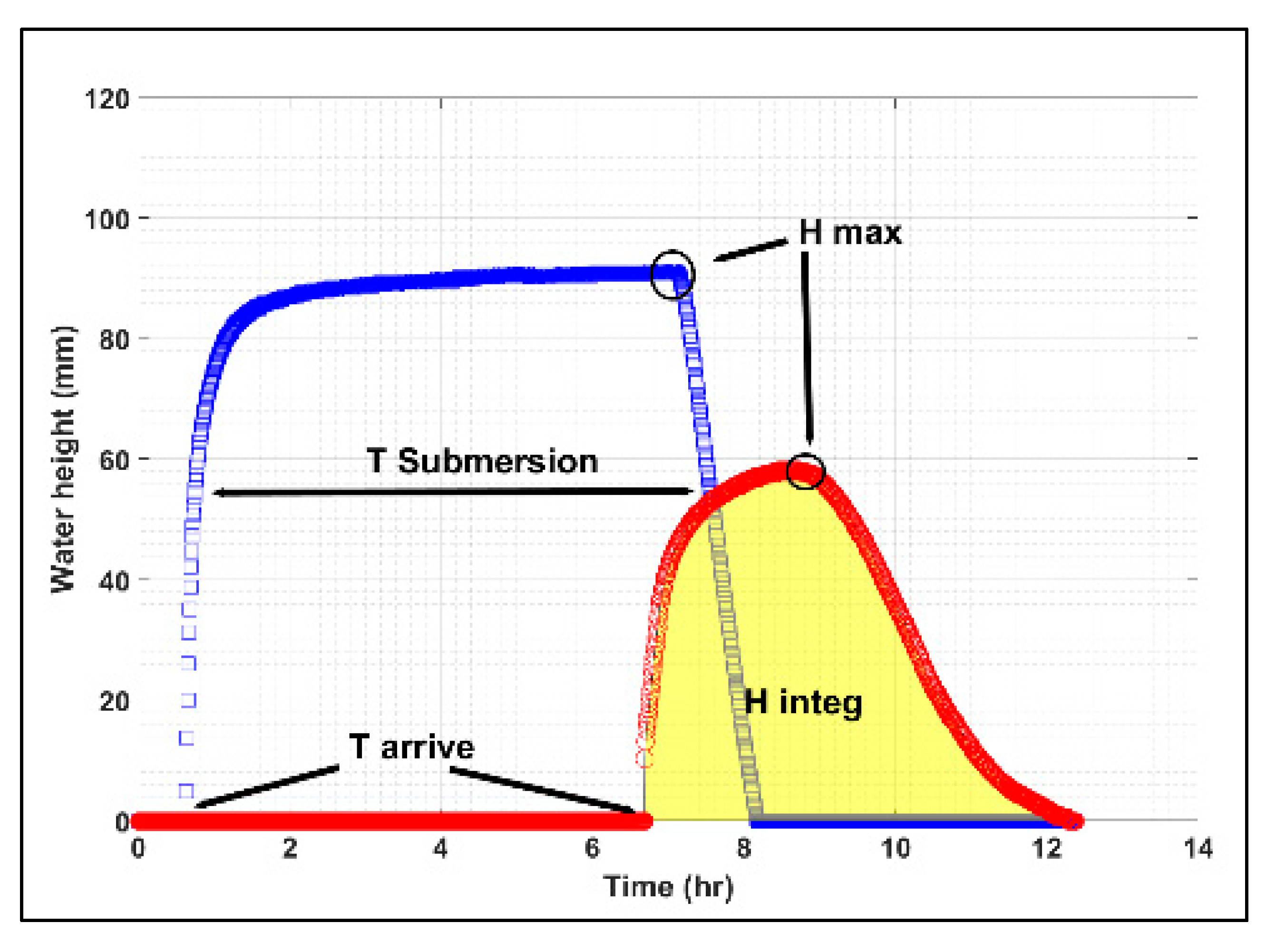
During each irrigation event, the evolution of the flow depth at the soil surface was measured with automatic probes and data loggers located at two cross sections of each plot. These sections were located at 10% (upstream section) and 90% (downstream section) of the total field length. Flow depth measurements were replicated three times at each section with Campbell Scientific CS616 probes, which were installed vertically with a 10 cm insertion into the soil. These probes, originally designed for soil moisture measurements, were calibrated and a linear relationship between the recorded signal of the probes, and the flow depth was obtained, with a mean R² of 0.99. As the length of the CS616 moisture probes is 30 cm, the maximum flow depth that could be measured was about 20 cm, the usual maximum flow depth obtained during flood irrigation of hay crops in the Crau area being about 10 cm. The probes were connected to a Campbell Scientific CR1000 data logger and measurements were made and stored every 30 s. The typical evolution of flow depth with time at the flow depth in the upstream and downstream sections that could be obtained is presented in Figure 2.

2.4. Measurement of Soil Characteristics

Soil samplings with augers were carried out before and after each event in order to determine the soil water content profile and the soil water depletion ∆θ. For each event, three replicates were obtained at the upstream section and three replicates at the downstream section. For each replicate, the soil samples were collected at three depths; 0–10 cm, 10–20 cm and 20–30 cm. Gravimetric water content was converted into volumetric water content using the measured bulk density of the fine earth between stones and was corrected according to the stone content.
The suction at the infiltration front, which is parameter Pini in the CALHY model, was not measured. Several authors [7,27,28] showed that Pini has only a slight influence on the simulation of the rates and the amounts of infiltration and streamflow depth compared to other parameters such as Ks, k and ∆θ. Moreover, as stated by [7], this parameter is closely related to the soil water depletion ∆θ and cannot change independently of ∆θ. Therefore, we decided to compute Pini from the soil water content depletion with the linear relation (R2 = 0.96) obtained from data presented by [7]:
P i n i = 54 × Δ θ + 0.4 ,
A typical value of Pini is 5.8 m, obtained for ∆θ = 0.1 m3·m−3. This value is higher than standards for textural class of [29] but was considered to be more precise than standards obtained from pedotransfer functions not adapted to our specific stony soils.

2.5. Measurement of Irrigation Characteristics

Inflow rate Qi was measured with OTT C2 current-meter. Equipped with a propeller fixed in front of the water current, it measures the velocity of the water flow with an accuracy of about ± 2%. The advancing surface water front was monitored for the two irrigation events: the observed position of the stream front was marked with plastic sticks every 30 minutes by an operator walking along the field at 5 locations in the cross section of the flow direction with plastic sticks. At the end of the experiment, the position of each plastic stick was measured with a decameter and a GPS device. The precision of the measurements was evaluated at ± 2 m. Photographic monitoring was also conducted to analyze the vegetation development (data not shown). The experimental dataset of the CALHY input parameters measured during each irrigation event is presented in Table 1.

2.6. Experimental Data Used for the Fitting Algorithm (“Proxy-Data”)

Key variables were extracted from the water depth hydrographs monitored at each data logger measurement (see Figure 2). We called them the “proxy-variables”. These variables are:
  • T_arrive (h) is the arrival time of the surface water front at each measurement location,
  • T_submersion (h) is the time interval between the arrival time and the end of the recession phase of the surface water front at a given measurement location in the field,
  • H_max (mm) is the maximum measured value of the flow depth,
  • H_integral (mm·h) is defined as: H i n t e g r a l = t a r r i v e t a r r i v e + t s u b m e r s i o n H ( t ) d t , computed directly using the trapezoidal method function.
These variables were calculated for the two measurement locations (10% of the plot length from the inlet for the 1st location and from the outlet for the 2nd one).

2.7. Inverse Modelling Approach

Based on the SIMPLEX algorithm [30], an inverse modeling approach was used to estimate parameters Ks, k, H0 and ∆θ of the CALHY model. The data used for the fit are the proxy-variables defined above. The objective function (OF) to be minimized was based on the weighted least squares method [31], computed as follows:
O F = j , l [ O b s j , l S i m j , l ( δ ) σ j ] 2 ,
where j is the variable number, l is the variable position, Obs and Sim are the observed and simulated variable values, δ is the vector of the sampled parameter values and σj2 is the variance of Obsj. The values of σj2 for each proxy variable were deduced from the experimental variance. They were calculated from the three signals recorded at each position in situ for each variable of interest.
As cited in [30,32], iteratively and independently, a set of parameters δ is sampled. The optimization scheme is based on evaluating the OF through successive iterations. For the first iteration an initial set of parameters’ values is sampled randomly inside a specified value range presented in Table 2. The accepted solution of an iteration (i), following the minimum OF, will replace the initial solution and will initial the next iteration (i+1) until achieving convergence. The convergence could be achieved when the maximum number of iterations has been reached or when the difference between two successive OF is less than a predefined tolerance criterion.
This optimization scheme is repeated 20 times with a maximum of 200 iterations and tolerance criterion cited to 0.001 for each one. It starts with a new set of initial parameter values within their interval limit. The final value of the parameters is the one corresponding to the minimum value of the objective function across all repetitions.

2.8. Evaluation of the Estimated Parameters

The evaluation of predictive capacity of the proposed approach was performed in three successive steps summarized in Table 3.

2.8.1. Coherence and Physical Meaning of the Fitted Parameters

The estimated value of physically-based parameters must fall within the range of expected values cited in the literature and their variations must be physically founded. Otherwise, it indicates a basic failure in the simulation of the processes involved in the surface irrigation event regardless of the quality of the calibration.
For a given field Ks is assumed to be constant over time as fields have not been tilled after the plantation of the meadows during the last several years. We therefore analyzed the variability of the value of Ks for one estimation to the other on each experimental site.
The coefficient k should be qualitatively related to the hay development and/or biomass: higher biomass leads to higher friction and thus a lower k. Moreover, the value of k should be less than the value for an agricultural bare soil: it should be maximal for an irrigation following the harvest of the field, and it should be minimal for the last irrigation just before the harvest.

2.8.2. Evaluation of the Simulated Hydrograph and Surface Water Front from Irrigation Events Used for Calibration

In a second step, we compared the predictions of the model to additional data measured during the same irrigation events but those data were not used for the calibration process. Large discrepancies between these two datasets would reveal that the proxy variables used in calibration process do not provide an exhaustive information on all the components of the processes involved in the surface irrigation. In that case, additional experimental data should be incorporated in the calibration process. Compared datasets which were not used in the inversion procedure include:
  • Estimated and the measured soil water depletion ∆θ
  • Simulated and monitored time flow depth hydrograph H(t) in two cross sections of the field
  • Simulated and monitored advancement of surface water front
Performance was evaluated using statistical indicators such as the root mean square error (RMSE) (see Equation 9) and the Nash-Sutcliffe criterion (see Equation (10)).
R M S E = i = 1 n ( X s i X o i ) 2 n ,
where Xs and Xo are the simulated and observed data, i.e., the flow depth (mm) for the water streamflow hydrograph or the advance distance measurements (m), both as a function of time;
C N a s h = 1 i = 1 n ( X s i X o i ) 2 i = 1 n ( X o ¯ X o i ) 2 ,
where X o ¯   is the mean of observed data.
The two first comparisons (∆θ and H(t)) were applied to all experiments where the parameters estimation by inversion was carried out, i.e., irrigations A1, A2, A3, A5, B6 and B7. The third comparison of the advance stream front was applied only for A5.

2.8.3. Evaluation of the Simulated Hydrograph and Surface Water Front for Cases Not Used for Calibration

In a third step, we compared the predictions of the model to the measured data obtained from independents irrigation events, which has not been included in the calibration process. Significant differences between model predictions and measurements would reveal a poor predictive capacity of the model to changes in irrigation conditions. This may also reveal a flawed representation of the physical processes in the model.
  • We simulated irrigation A4 that was not used during the calibration process. Parameters Ks, k, H0 and ∆θ used for this direct simulation were derived from the parameters obtained from irrigation A5. The comparison between the simulated and measured data was performed upon the advancement of the surface water and the water depth hydrographs H(t) at the two selected sections of the field.
  • Two irrigation experiments referred to in [5] were obtained. They were monitored in the first experimental site and labelled irrigation A6 and A7. The first one occurred after the 1st mowing with a leaf area index (LAI) of about 1.3 and similar to those of irrigation A3 in our dataset. The second occurred before the 2nd mowing: the development of the vegetation was maximum with a LAI of about 7.7 and similar to that of irrigation A2. Therefore, we used the parameters fitted on irrigation A3 and A2 to simulate outputs of irrigation A6 and A7 respectively.
  • Overall compared data for validation were also evaluated with RMSE and Nash criterion.

3. Results and Discussion

This section discusses the ability of the proposed inversion system to predict the identified proxy variables by fitting the parameters k, Ks, H0 and ∆θ. These parameters were fitted for the irrigation events A1, A2, A3, A5, B6 and B7 with their values are listed in Table 4.

3.1. Coherence and Physical Meaning of the Fitted Parameters

Results show that for a given experimental site, the fitted value of Ks did not change from one irrigation experiment to another. For the first site, values of Ks varied within a very narrow range between 1.34 × 10⁶ and 1.5 × 10⁻⁶ m·s−1. This parameter value varied within a very narrow range. An average value of 1.4 × 10⁻⁶ m·s−1 was calculated for this site, which is in accordance with the values obtained by [5,7] for the same plot. For the second site, the two estimations of Ks were also close to each other, with an average value of 1.1 × 10⁷ m·s−1. This result indicates that the soil of the second experimental site may be less permeable than the soil of the first site. The soil characteristics of the second site which is hydromorphic and has a higher clay content and a higher organic content [26].
For both experimental sites, the estimated value of k ranged between 1.65 and 3.54 m1/3·s−1. [7] calculated by inversion the value of k for the same based on six irrigations events. They found that k varied from 2.4 to 5.3 m1/3·s−1. [33] assessed the variation of parameter k in furrows under different conditions and found that k ranged between 8 and 16 m1/3·s−1. They showed that it could reduce by up to 30% when the vegetation increased by 47%. [34] suggested a value of k between 2.2 and 3.7 m1/3·s−1; [35] suggested a value of k ranging from 3.3 to 6.7 m1/3·s−1 for a field planted with alfalfa and irrigated with border irrigation. [36] found that k varied from 2.8 to 5 m1/3·s−1 for a field sown with perennial pasture. In conclusion, our fitted values of k agree well with the values found in the literature.
For the second site, the values of k were close to 1.65 m1/3·s−1, which is significantly less than the values derived for the first site. From a hydraulic point of view, the effect of the hydraulic friction of on the flow advancement increases as the irrigation rate and flow rate decrease [33,37]; The field surface and vegetation stage in the second experimental site were close to those in the first one, but the applied rates during the irrigation experiments B6 and B7 were 50% lower than those applied in A1, A2 and A3 and 30% lower than in that applied A4 and A5, this justifies the lower k value.
For the parameter H0, it is difficult to assess the coherence of the estimated results due to the difficulty in measuring this parameter. The simulated values of this parameter reported in [38,39] ranged from 0 mm to 30 mm and from 0.26 to 48.0 mm respectively. For a random soil roughness, the slope is expected to reduce the soil surface storage [40], whereas the vegetation is expected to increase this value [41]. For our experimental conditions, the soil was very flat with a very smooth microrelief, as the soil was leveled several years ago and was never tilled. Therefore, a lower value of H0 is expected, which is the case.

3.2. Evaluation of the Performance of the Proposed Approach for Parameter Estimation

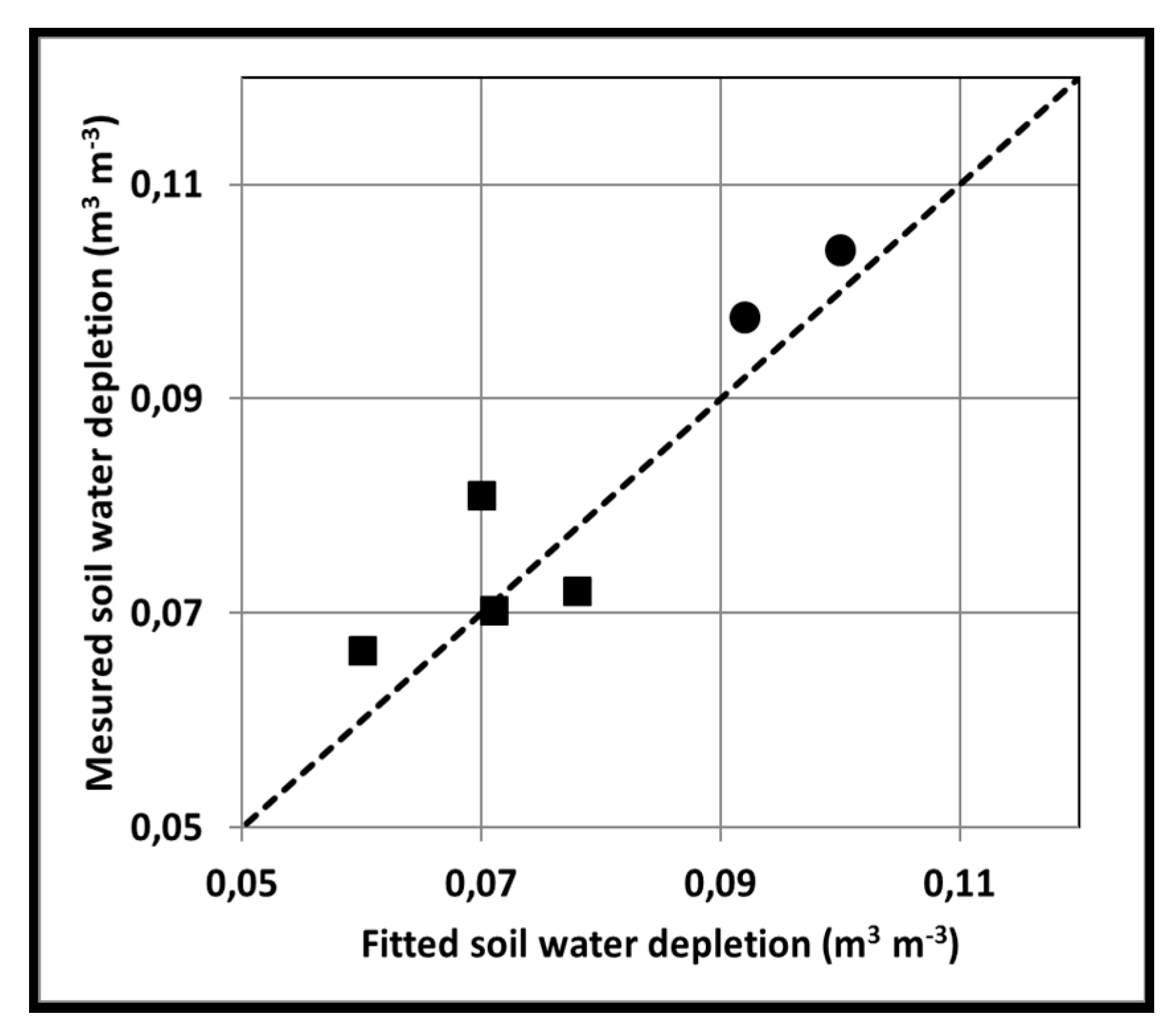
Fitted values and measured values of ∆θ are shown in Figure 3, they range between 0.07–0.104 m3·m−3, and 0.06–0.1 m3·m−3 respectively, which is quite very low. This is due to the high content of stones with a very low porosity in the soil profile. The correlation coefficient between the two is R² = 0.85, points are distributed near the 1:1 line except one point.
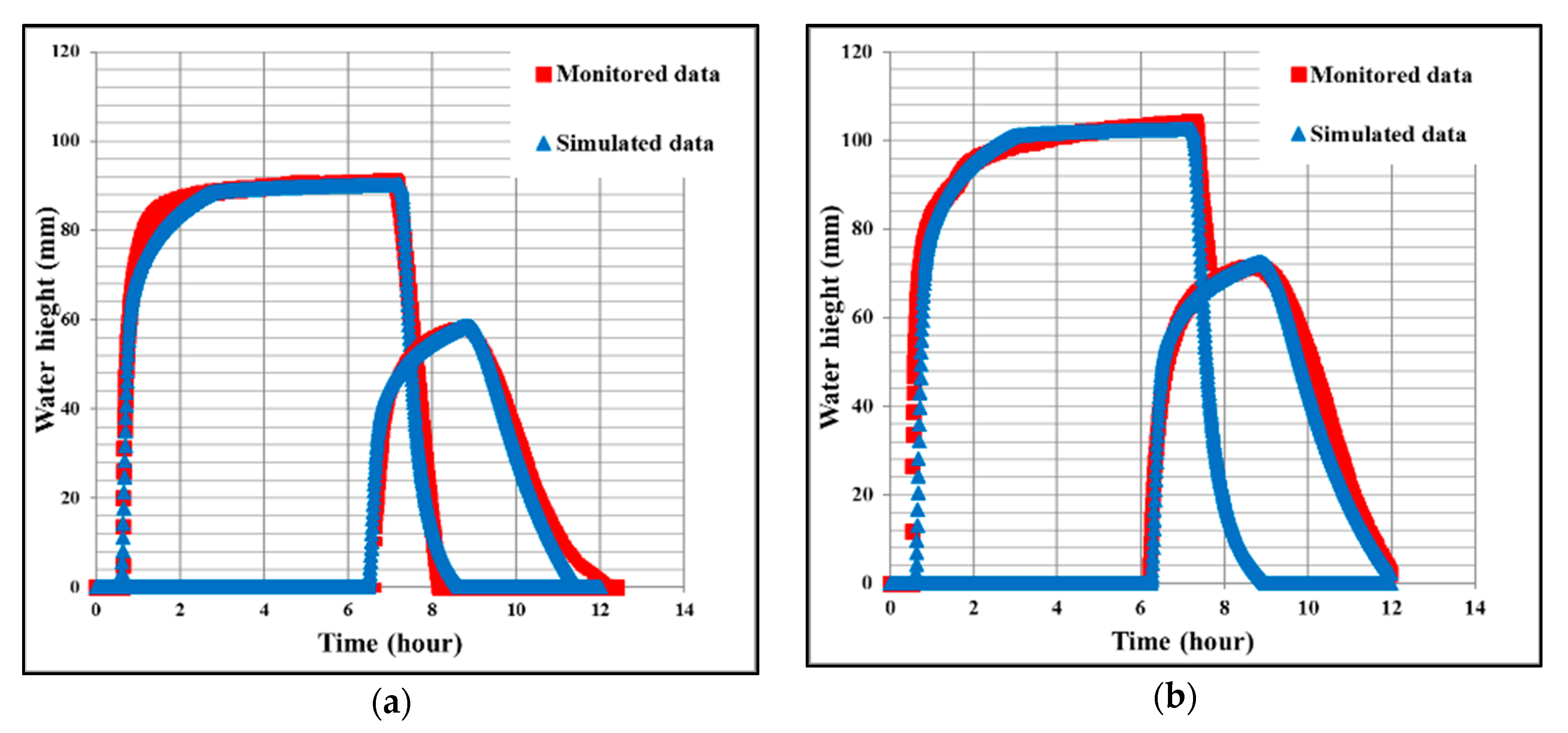
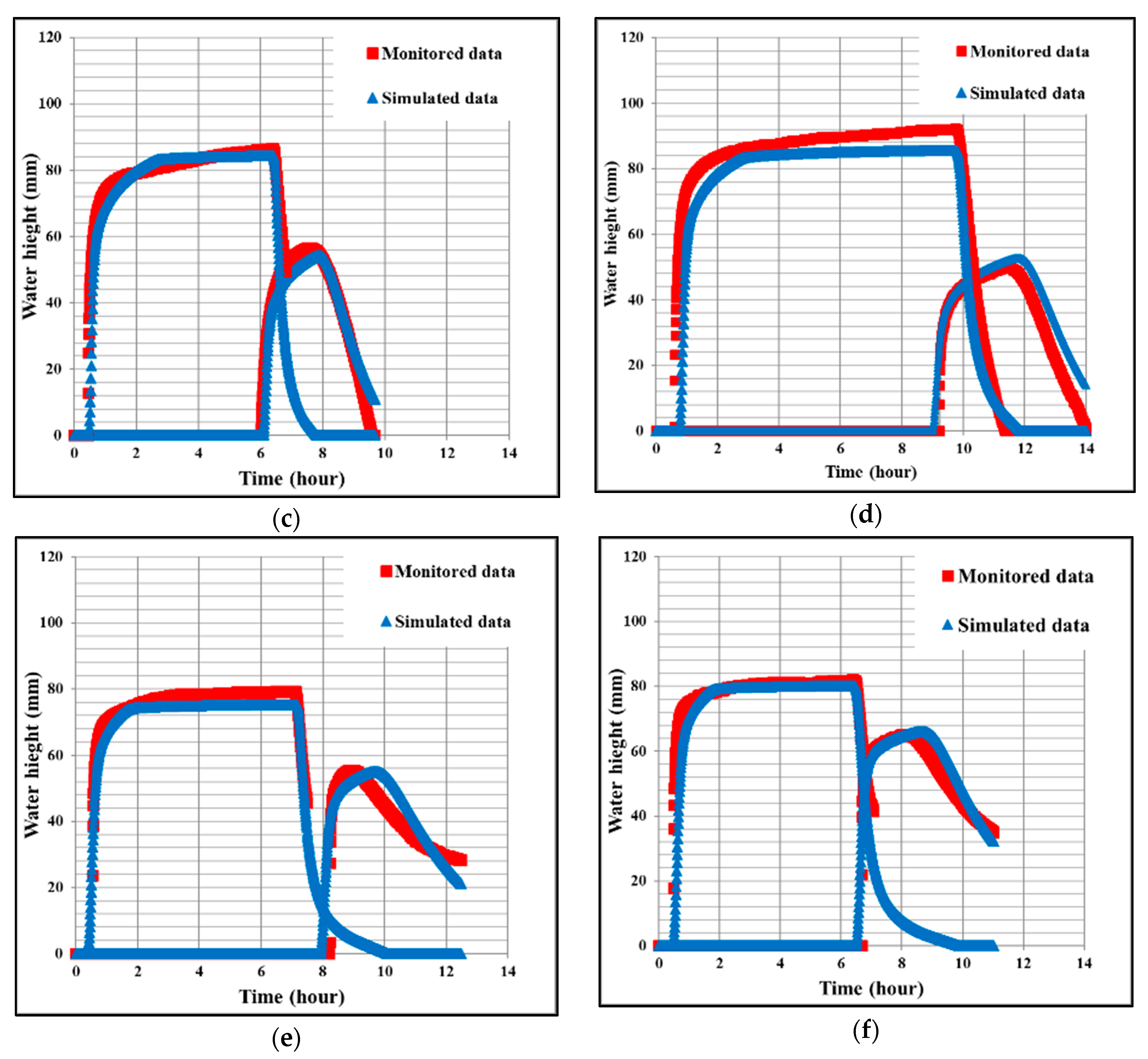
The results show that the predicted and observed streamflow hydrographs have a good agreement in all simulated cases. The Nash criterion was always higher than 0.85 for the upstream section and was close to 1.00 for the downstream section. The maximum value of the RMSE criteria in the upstream section was 10.12 mm for A2 whereas the lowest value was 3.6 mm for A1. At the downstream section was close to 3 mm for all irrigation experiments. The results of the comparison between the simulated and observed hydrographs are presented in Figure 4. The estimated RMSEs and Nash criteria are presented in Table 5.
Figure 5 shows excellent agreement between the modelled and observed surface water advancement monitored during experiment A5. The Nash criterion was close to 1 and the RMSE value was close to 6 m.

3.3. Evaluation of the New Parameter Estimation Approach

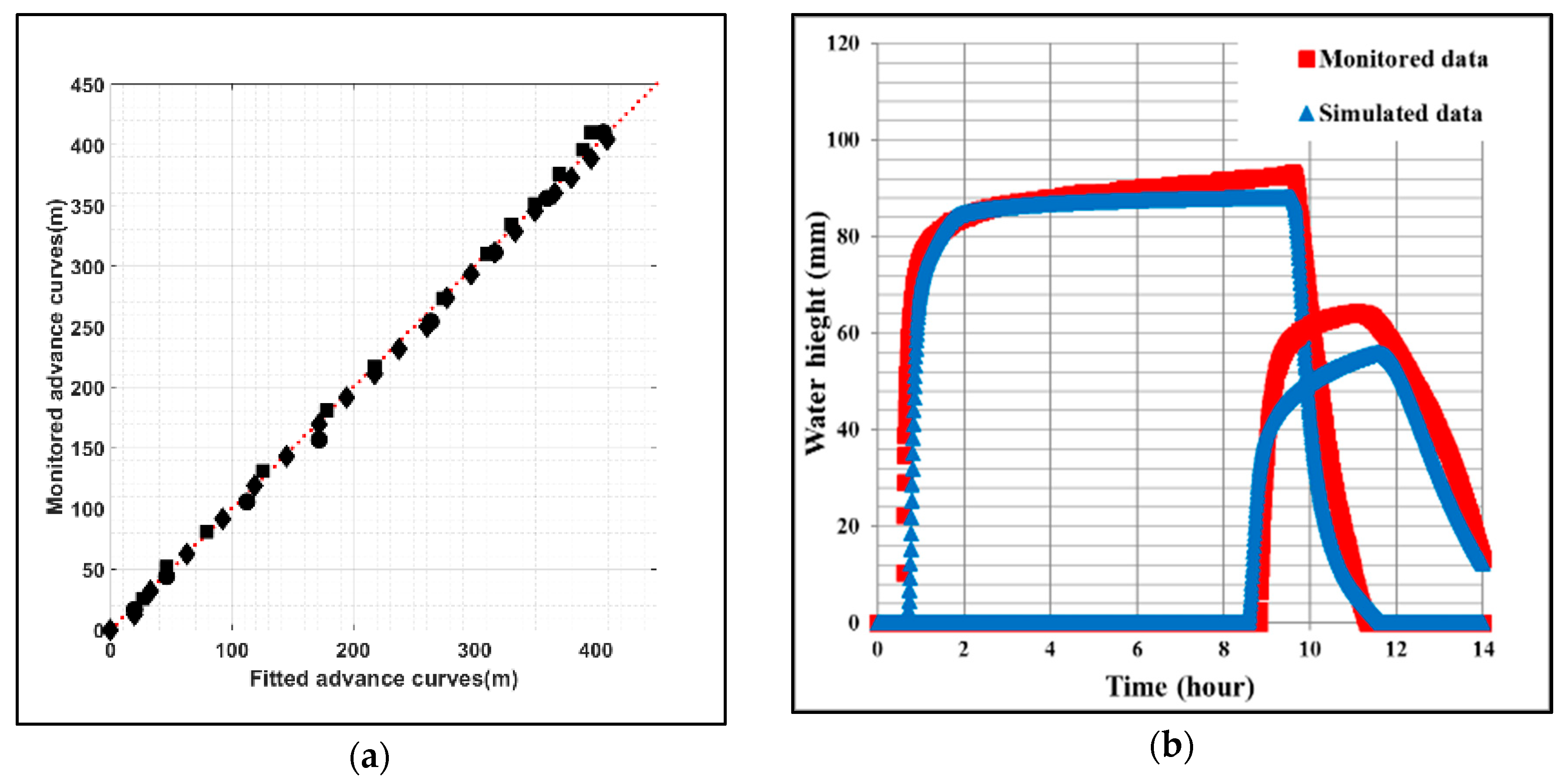
All data are presented in Figure 6 and Table 6. Table 6 shows that the simulated data are in very good agreement with the observed data.
The Nash criterion CNASH calculated using the advance curve data is close to 1 and it is higher than 0.9 when calculated with the hydrograph data. The RMSE value is about 6 m for the advance curve and between 6 mm and 9 mm for the hydrograph. The values of CNASH and RMSE calculated for the validation experiments are very close to the ones calculated for the verification experiments, which validates our proposed methodology for the estimation of both soil hydrodynamic parameters and soil surface hydraulic parameters.

4. Conclusions

The main objective of this study was to develop an improved method able to estimate soil hydrodynamic parameters and soil surface hydraulic parameters at the field scale. It was performed by coupling an inverse modelling approach with flood irrigation measurements: two sets of easy proxy variables measured upstream and downstream parts of the irrigated field. In addition to the ease and accessibility of the proposed variables, they deliver sufficient information to estimate the soil parameters with a high accuracy.
The performance of the proposed method was thoroughly evaluated in three steps. The first step was dedicated to studying the physical meaning of the fitted parameters for six different irrigation events. The second step was dedicated to verify the inverse modelling approach. We used additional data that has not been incorporated into the fitting (calibration) process. These data were obtained during the same irrigations as the ones used for the inverse modelling. Error criteria such as the Nash coefficient and the RMSE were calculated. The final evaluation was carried out using observed data obtained from independents irrigation experiments. The same error criteria were calculated and were similar to those calculated during the verification step. To our knowledge, and as far as surface irrigation is concerned, this is the first time that such a fitting process has been evaluated in three successive steps and with data obtained from other authors.
Results showed that the proposed method is robust and effective in estimating the saturated hydraulic conductivity Ks, the Manning-Strickler roughness coefficient k and the soil water depletion ∆θ with a high degree of accuracy. The soil surface depressional storage coefficient H0 was estimated with a large uncertainty. Nevertheless, this parameter has only a slight effect on the irrigation dynamics and the water balance at the field scale during one irrigation.
The improvement of parameter estimation proposed in this paper could be achieved by identifying some additional experimental variables. Based upon their incorporation in the objective function, a global sensitivity analysis could help in the identification of the kind, the number and the location in the field of these new variables [4,42].
Hence, the predictive capacity of the model, associated with the proposed calibration method, has been validated. The proposed methodology proved to perform well in estimating the main soil parameters governing flood during the irrigation of hay fields. These parameters can then be used in the CALHY surface flow-infiltration model [7] first to analyze current irrigation practices. Consequently, methods of irrigation optimization can be proposed in order to increase the water efficiency of surface irrigation systems, and hence save water. Moreover, this methodology can easily be implemented over large irrigated areas. Thereby, soil parameters mapping could be developed (hydraulic conductivity, hydraulic roughness and soil water availability) at the field scale when border irrigation technology is used.

Author Contributions

Conceptualization, data curation and writing: S.R., M.A.A.; Resources: S.B., F.C., M.A.A., S.R.; Software: S.B., P.L., M.A.A.; J.C.B.; Formal analysis, validation: S.B., P.L., M.A.A.; Supervision, review and editing: S.R., A.O.

Funding

This work was partly funded by the SICMED program of the French initiative MISTRALS (Mediterranean Integrated STudies at Regional and Local Scales).

Acknowledgments

The authors wish to thank farmers from the Crau region for providing access to their fields and all the technical staff of UMR EMMAH for their help during the irrigation monitoring.

Conflicts of Interest

The authors declare that they have no conflict of interest.

References

  1. FAO. AQUASTAT Main Database, Food and Agriculture Organization of the United Nations (FAO 2016). Available online: http://www.fao.org/nr/water/aquastat/main/index.stm (accessed on 3 June 2016).
  2. Clemmens, A.J. Errors in Surface Irrigation Evaluation from Incorrect Model Assumptions. J. Irrig. Drain. Eng. 2009, 135, 556–565. [Google Scholar] [CrossRef]
  3. Moravejalahkami, B.; Mostafazadeh-Fard, B.; Heidarpour, M.; Abbasi, F. Furrow infiltration and roughness prediction for different furrow inflow hydrographs using a zero-inertia model with a multilevel calibration approach. Biosyst. Eng. 2009, 103, 374–381. [Google Scholar] [CrossRef]
  4. Varella, H.; Buis, S.; Launay, M.; Guérif, M. Global sensitivity analysis for choosing the main soil parameters of a crop model to be determined. Agric. Sci. 2012, 3, 949–961. [Google Scholar] [CrossRef]
  5. Mailhol, J.C.; Merot, A. SPFC: A tool to improve water management and hay production in the Crau region. Irrig. Sci. 2008, 26, 289–302. [Google Scholar] [CrossRef] [Green Version]
  6. Bautista, E.; Clemmens, A.J.; Strelkoff, T.S.; Schlegel, J. Modern analysis of surface irrigation systems with WinSRFR. Agric. Water Manag. 2009, 96, 1146–1154. [Google Scholar] [CrossRef]
  7. Bader, J.C.; Saos, J.L.; Charron, F. Model of border irrigation runoff, advance and infiltration on a soil covering a very permeable subsoil. Hydrol. Sci. J. 2010, 55, 177–191. [Google Scholar] [CrossRef]
  8. Gillies, M.H.; Smith, R.J. SISCO: Surface irrigation simulation, calibration and optimisation. Irrig. Sci. 2015, 33, 339–355. [Google Scholar] [CrossRef]
  9. Cahoon, J. Kostiakov infiltration parameters from kinematic wave model. J. Irrig. Drain. Eng. 1998, 124, 127–130. [Google Scholar] [CrossRef]
  10. Sedaghatdoost, A.; Ebrahimian, H. Calibration of infiltration, roughness and longitudinal dispersivity coefficients in furrow fertigation using inverse modelling with a genetic algorithm. Biosyst. Eng. 2015, 136, 129–139. [Google Scholar] [CrossRef]
  11. Amoah, J.K.O.; Amatya, D.M.; Nnaji, S. Quantifying watershed surface depression storage: Determination and application in a hydrologic model. Hydrol. Process 2013, 27, 2401–2413. [Google Scholar] [CrossRef]
  12. Elliott, R.L.; Walker, W.R. Field evaluation of furrow infiltration and advance functions [irrigation; Colorado]. Trans. ASAE 1982, 25, 396–400. [Google Scholar] [CrossRef]
  13. Gillies, M.H.; Smith, R.J. Infiltration parameters from surface irrigation advance and run-off data. Irrig. Sci. 2005, 24, 25–35. [Google Scholar] [CrossRef] [Green Version]
  14. Walker, W.R. Multilevel calibration of furrow infiltration and roughness. J. Irrig. Drain. Eng. 2005, 131, 129–136. [Google Scholar] [CrossRef]
  15. Green, W.H.; Ampt, G.A. Studies on soil physics: The flow of air and water through soils. J. Agric. Sci. 1911, 4, 1–24. [Google Scholar]
  16. Bautista, E.; Strelkoff, T.S.; Clemmens, A.J. Improved Surface Volume Estimates for Surface Irrigation Volume-Balance Calculations. J. Irrig. Drain. Eng. 2012, 138, 715–726. [Google Scholar] [CrossRef]
  17. Bautista, E.; Schlegel, J.L. A flexible system for estimation of infiltration and hydraulic resistance parameters in surface irrigation. Trans. ASABE 2017, 60, 1223–1234. [Google Scholar] [CrossRef]
  18. Ebrahimian, H.; Liaghat, A.; Ghanbarian-Alavijeh, B.; Abbasi, F. Evaluation of various quick methods for estimating furrow and border infiltration parameters. Irrig. Sci. 2010, 28, 479–488. [Google Scholar] [CrossRef]
  19. Gillies, M.H.; Smith, R.J.; Raine, S.R. Accounting for temporal inflow variation in the inverse solution for infiltration in surface irrigation. Irrig. Sci. 2006, 25, 87–97. [Google Scholar] [CrossRef] [Green Version]
  20. Mailapalli, D.R.; Wallender, W.W.; Raghuwanshi, N.S.; Singh, R. Quick method for estimating furrow infiltration. J. Irrig. Drain. Eng. 2008, 134, 788–795. [Google Scholar] [CrossRef]
  21. Shepard, J.S.; Wallender, W.W.; Hopmans, J.W. One-point method for estimating furrow infiltration. Trans. ASAE 1993, 36, 395–404. [Google Scholar] [CrossRef]
  22. Katopodes, N.K. Observability of surface irrigation advance. J. Irrig. Drain. Eng. 1990, 116, 656–675. [Google Scholar] [CrossRef]
  23. Weibo, N.; Liangjun, F.; Xiaoyi, M. Estimated Infiltration Parameters and Manning Roughness in Border Irrigation. Irrig. Drain. 2012, 61, 231–239. [Google Scholar] [CrossRef]
  24. Buis, S.; Wallach, D.; Guillaume, S.; Varella, H.; Lecharpentier, P.; Launay, M.; Guérif, M.; Bergez, J.E.; Justes, E. The STICS Crop Model and Associated Software for Analysis, Parameterization, and Evaluation. In Methods of Introducing System Models into Agricultural Research; American Society of Agronomy: Madison, SD, USA, 2011. [Google Scholar]
  25. Merot, A.; Wery, J.; Isberie, C.; Charron, F. Response of a plurispecific permanent grassland to border irrigation regulated by tensiometers. Eur. J. Agron. 2008, 28, 8–18. [Google Scholar] [CrossRef]
  26. Bouteyre, G.; Duclos, G. Carte Pédologique de la France à 1/100000; INRA: Arles, France, 1994. [Google Scholar]
  27. Galbiati, G.; Savi, F. Evaluation of the comparative influence of soil hydraulic properties and roughness on overland flow at the local scale. J. Agric. Eng. Res. 1995, 61, 183–190. [Google Scholar] [CrossRef]
  28. Risse, L.M.; Nearing, M.A.; Savabi, M.R. Determining the Green-Ampt effective hydraulic conductivity from rainfall-runoff data for the WEPP model. Trans. ASAE 1994, 37, 411–418. [Google Scholar] [CrossRef]
  29. Rawls, W.J.; Brakensiek, D.L.; Saxton, K.E. Estimation of soil water properties. Trans. ASAE 1982, 25, 1316–1320. [Google Scholar] [CrossRef]
  30. Nelder, J.A.; Mead, R. A Simplex Method for Function Minimization. Comput. J. 1965, 7, 308–313. [Google Scholar] [CrossRef]
  31. Charnes, A.; Frome, E.L.; Yu, P.-L. The equivalence of generalized least squares and maximum likelihood estimates in the exponential family. J. Am. Stat. Assoc. 1976, 71, 169–171. [Google Scholar] [CrossRef]
  32. Lagarias, J.C.; Reeds, J.A.; Wright, M.H.; Wright, P.E. Convergence Properties of the Nelder-Mead Simplex Algorithm in Low Dimensions. SIAM J. Optim. 1998, 9, 112–147. [Google Scholar] [CrossRef]
  33. Rasoulzadeh, A.; Sepaskhah, A.R. Scaled Infiltration Equations for Furrow Irrigation. Biosyst. Eng. 2003, 86, 375–383. [Google Scholar] [CrossRef]
  34. Michael, A.M. Irrigation: Theory and Practice; Vikas Publishing House Pvt Ltd.: Noida, India, 2009. [Google Scholar]
  35. Davis, C.A.; Collins, H.G.; Portland, O.R.; Woodward, G.; Humpherys, A.S.; Hart, W.E. Design and Operation of Farm Irrigation Systems; The American Society of Agricultural and Biological Engineers: Joseph, MI, USA, 1980. [Google Scholar]
  36. Robertson, D.; Wood, M.; Wang, Q.J. Estimating hydraulic parameters for a surface irrigation model from field conditions. Aust. J. Exp. Agric. 2004, 44, 173–179. [Google Scholar] [CrossRef]
  37. Khattabi, A.A.; Hablous, A.A.; Elnemry, M.M. The Relation between the Coefficient of Friction and Pressure Drop by Using the Different Reynolds Number in a Circular Tube. J. Fluid Dyn. 2015, 5, 99–105. [Google Scholar] [CrossRef]
  38. Kamphorst, E.C.; Jetten, V.; Guérif, J.; Iversen, B.V.; Douglas, J.T.; Paz, A. Predicting depressional storage from soil surface roughness. Soil Sci. Soc. Am. J. 2000, 64, 1749–1758. [Google Scholar] [CrossRef]
  39. Kamphorst, E.C.; Duval, Y. Validation of a numerical method to quantify depression storage by direct measurements on moulded surfaces. Catena 2001, 43, 1–14. [Google Scholar] [CrossRef]
  40. Álvarez-Mozos, J.; Campo, M.Á.; Giménez, R.; Casalí, J.; Leibar, U. Implications of scale, slope, tillage operation and direction in the estimation of surface depression storage. Soil Till. Res. 2011, 111, 142–153. [Google Scholar] [CrossRef]
  41. Paz-Ferreiro, J.; Bertol, I.; Vidal Vázquez, E. Quantification of tillage, plant cover, and cumulative rainfall effects on soil surface microrelief by statistical, geostatistical and fractal indices. Nonlinear Process. Geophys. 2008, 15, 575–590. [Google Scholar] [CrossRef] [Green Version]
  42. Tiscareno-Lopez, M.; Lopes, V.L.; Stone, J.J.; Lane, L.J. Sensitivity analysis of the WEPP watershed model for rangeland applications I: Hillslope processes. Trans. ASAE 1993, 36, 1659–1672. [Google Scholar] [CrossRef]
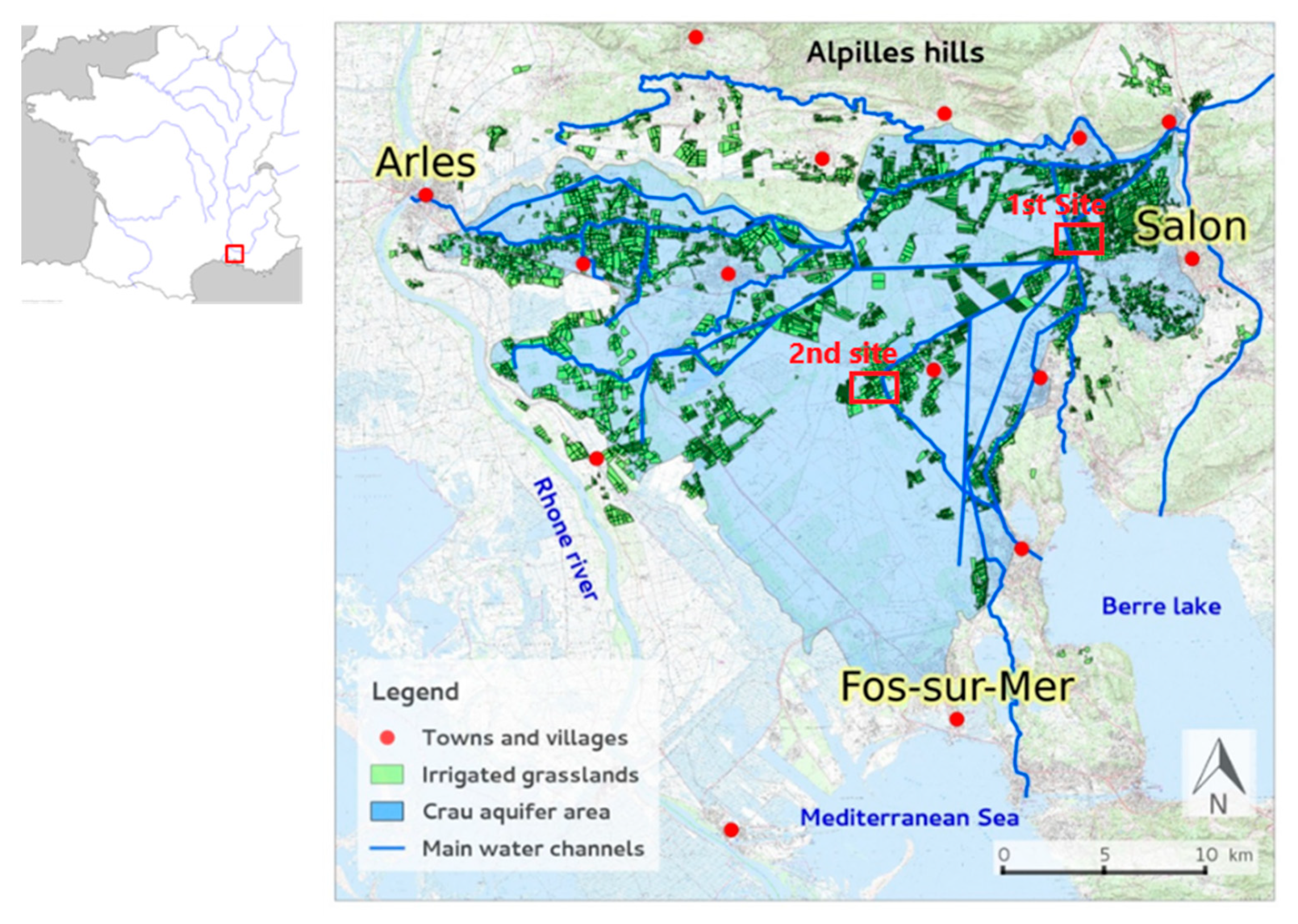
Figure 1. Map of the Crau area showing the aquifer limits, the irrigated grassland areas including the two monitored sites and the main surface water channels.
Water 10 01581 g001
Figure 2. Time evolution of water levels during an irrigation event in two locations monitored in the 1st site. The first blue curve was obtained in the upstream section of the field, and the second red curve in the downstream section of the field. Proxy-variables used in fitting process are given on this figure.
Water 10 01581 g002
Figure 3. Comparison between fitted (X-axis) and measured (Y-axis) soil water depletion in the two experimental sites and for all irrigations used during the fitting process. The continuous line is the 1:1 line, black squares are for the first site, black circles are for the second site.
Water 10 01581 g003
Figure 4. Comparison between simulated (blue triangles) and measured (red squares) water depth hydrographs in the upstream and downstream sections of the field. Simulations were performed with the fitted set of soil parameters. On each figure the first curve (on the left part of the X-axis) was obtained on the upstream section, whereas the second curve (on the right part of the X-axis) was obtained on the downstream section. (a) is for irrigation A1; (b) for irrigation A2; (c) for irrigation A3, (d) for irrigation A5; (e) for irrigation B6 and (f) for irrigation B7.
Water 10 01581 g004aWater 10 01581 g004b
Figure 5. Comparison of measured and simulated advance curves of the surface water front for irrigation A5. The continuous line in red is the 1:1.
Water 10 01581 g005
Figure 6. Third step of the validation of the fitting process using independent measurement. In (a) comparison of simulated and measured advance curves of the stream front: data presented with square and circle are for irrigations A6 and A7 studied by [5] respectively; data presented with diamond are those of irrigation A4. Simulations in A6 and A7 were performed with the fitted set of soil parameters in A3 and A2 respectively following the vegetation conditions; (b) is the comparison between simulated (blue triangle) and measured (red squares) surface water flow hydrographs in the upstream (first curve on the left) and downstream (second curve on the right) sections of the field during irrigation A4. Simulations were performed with the fitted parameters of A5.
Water 10 01581 g006
Table 1. Datasets for the monitored experimental irrigations. N is the label of the irrigation, L is the field length, W is the field width, I is the field slope, Q is the irrigation discharge per unit width of the field, ∆θ is the soil water depletion, Z is the soil depth, Ti is the irrigation duration, Date is the date of the irrigation relative to the mowing date of the field.
NLW
(m)
I
(‰)
Q
(L·s−1·m−1)
θ
(m3·m−3)
Z
(mm)
Ti
(h)
Date
(m)
1st siteA1410492.82.850.0704507.1610 days before 1st mowing
A230.0667.1548 days before 2nd mowing
A33.020.0726.3510 days after a 2nd mowing
A42.280.0729.521 days after a 2nd mowing
A52.080.0819.6831 days after a 2nd mowing
2nd siteB6604.81.480.0972007.1220 days after a 2nd mowing
B71.650.1036.4539 days after a 2nd mowing
Table 2. Boundary values of each parameter of interest. Initial values of each parameter are drawn within these boundary values at the beginning of the fitting process.
log [KS (m·s−1)]k (m·s−1/3)∆θ (m3·m−3)H0
Min−7.21.50.060
Max−5.64.50.1220
Table 3. The three steps of the evaluation strategy of the fitting process. Step one (“coherence”) is used to check the physical meaning of the fitted parameters; step two (“evaluation with experiments used for the inverse modelling”) is a “weak validation” performed on data which were not used in the inversing process; Step three (“evaluation with experiments had not submitted in the inverse modelling”) is the validation sensu stricto.
ExperimentCoherence of Fitted ParametersEvaluation with Data Didn’t Used in Fitting ProcessEvaluation Using Data from Independent Experiments
A1, A2, A3, A5, B6, B7- Temporal Stability of Ks- Measured/fitted ∆θ.
- f (Hay development, k).- Measured/simulated H(t)
A5 - Measured/simulated streamflow advance curve.
A4, A6, A7 [5] - H(t) in A4 simulated with fitted parameters from A5
- Streamflow advance curve in A4, A6 and A7 using fitted parameters from A5, A3 and A2 respectively.
Table 4. Irrigation parameters estimated for the different irrigations. Fitted values +/− one square root of the variance are given in brackets.
A1A2A3A5B6B7
Ks (m·s−1)1.5 × 10⁻⁶
(1.08–2.07) × 10−6
1.34 × 10⁻⁶
(0.9–1.99) × 10−6
1.36× 10⁻⁶
(0.98–1.88) × 10−6
1.41× 10⁻⁶
(0.94–2.1) × 10−6
1.15× 10⁻⁷
(0.83–1.59) × 10−7
1.11× 10⁻⁷
(0.8–1.53) × 10−7
k (m·s−1/3)2.94
(2.43–3.44)
2.61
(2.15–3.06)
3.54
(3.15–3.92)
2.53
(1.99–3.06)
1.69
(1.58–1.79)
1.65
(1.45–1.85)
θ (m3·m−3)0.071
(0.05–0.09)
0.06
(0.04–0.08)
0.078
(0.06–0.09)
0.07
(0.05–0.09)
0.1
(0.08–0.12)
0.092
(0.07–0.11)
H0 (mm)0.3
(0–6.3)
1.9
(0–5.6)
2.6
(0–6.13)
4.2
(0–10.2)
3.3
(0–7.1)
2.6
(0–4.8)
Table 5. Values of the performance criteria calculated during the verification step of the fitting process. CNASH is the Nash criterion. RMSE is the Root Mean Square Error between simulated and measured data.
ExperimentsA1A2A3A5B6B7
Cnash (−) Upstream0.990.850.860.890.850.96
Downstream0.971.000.980.940.980.94
RMSE (mm)Upstream3.6310.128.1810.298.614.13
Downstream3.781.573.414.633.554.74
Table 6. Values of the performance criteria calculated during the validation step of the fitting process. CNASH is the Nash criterion. RMSE is the Root Mean Square Error between simulated and measured data. RMSE units are m for the advance curve and mm for the hydrograph.
Streamflow Advanced CurveStreamflow Hydrograph
ExperimentsA4A6A7UpstreamDownstream
CNASH (−)1.001.001.000.900.95
RMSE (m)5.105.387.328.965.86