Deep Learning with a Long Short-Term Memory Networks Approach for Rainfall-Runoff Simulation

Abstract

Considering the high random and non-static property of the rainfall-runoff process, lots of models are being developed in order to learn about such a complex phenomenon. Recently, Machine learning techniques such as the Artificial Neural Network (ANN) and other networks have been extensively used by hydrologists for rainfall-runoff modelling as well as for other fields of hydrology. However, deep learning methods such as the state-of-the-art for LSTM networks are little studied in hydrological sequence time-series predictions. We deployed ANN and LSTM network models for simulating the rainfall-runoff process based on flood events from 1971 to 2013 in Fen River basin monitored through 14 rainfall stations and one hydrologic station in the catchment. The experimental data were from 98 rainfall-runoff events in this period. In between 86 rainfall-runoff events were used as training set, and the rest were used as test set. The results show that the two networks are all suitable for rainfall-runoff models and better than conceptual and physical based models. LSTM models outperform the ANN models with the values of $R^2$ and $NSE$ beyond 0.9, respectively. Considering different lead time modelling the LSTM model is also more stable than ANN model holding better simulation performance. The special units of forget gate makes LSTM model better simulation and more intelligent than ANN model. In this study, we want to propose new data-driven methods for flood forecasting.

1. Introduction

Flooding always carries a lot of debris and waste like dead animal bodies and hazardous materials. The debris could make serious threats to mankind’s health and could destroy reservoirs and roads worsening the situation. The best way to cope with these issues is to build flood management systems for the decision-making process of critical situations [1,2]. In hydrological processes, rainfall is taken major components and decided the drought or flooding events. Recently, there are mainly three types of models for simulating the relationship of rainfall and runoff [3,4]:conceptual models, physical-based models and black box models. A conceptual model is a representation of a system, made of the composition of concepts which are used to help us to know, understand, or simulate a subject the model represents [5]. A physical-based model is a smaller or larger physical copy of an object to study hydrological process [6]. A black box model is a system which can be viewed in terms of its inputs and outputs without any knowledge of its internal working [7].

With accurate modelling of rainfall-runoff dynamics, it could not only provide a flood warning to reduce hazards but also enhance proper reservoirs management during the drought periods. However, it is difficult to fully understand the relationship between precipitation and runoff. It is because of temporal and spatial variability of basin characteristics, rainfall, coverage of vegetation, as well as factors in the rainfall-runoff process such as physical-based distributed hydrological model. Therefore, rainfall-runoff modelling is a hot field of study in hydrology research [8].

Among these three types of models, the conceptual and physical maybe the best two models to understand the process of rainfall-runoff. While these models also need more basin parameters like soil moisture, soil type, slope, shape, topography, temperature, evapotranspiration. The different watershed parameters also contain very complex relationships to construct these models [9]. Besides, In the rural region it is hard to get these watershed parameters. Therefore, black models have been increasingly emphasized during these years again [10].

These black box models are used more and more as the data-driven techniques are developing [11]. The Artificial Neural Networks (ANN), one of the data-driven techniques, have been widely used in hydrology as an alternative to physical-based and conceptual models [12,13]. These ANN techniques are based on artificial intelligence (AI), which is among the most famous skills in recent years. These skills could capture non-linearity and non-stationarity related to hydrological applications. Thus, data-driven methods based on AI have gained more attention for rainfall-runoff simulation [14].

In the last two decades, AI has been widely used for efficient simulating of nonlinear systems and capturing noise complexity in the datasets. For example, ANN and fuzzy logic are two popular AI-based approaches in flood prediction. Comparing with the classical black box models such as Auto Regressive (AR), Moving Average (MA), Auto Regressive Moving Average (ARMA), Auto Regressive Integrated Moving Average (ARIMA), Auto Regressive Integrated Moving Average with exogenous input (ARIMAX), Linear Regression (LR), and Multiple Linear Regression (MLR) which are linear, AI-based models are nonlinear models which are able to capture non-stationarity and non-linearity features. As a result, more and more researchers have developed models that are able to overcoming the drawbacks of conventional models [15].

In the above, conventional machine learning techniques only have the ability to process natural data in their raw form without other insight information. However, Deep learning allows computational models that are composed of multiple processing layers to learn representations of data with multiple levels of abstraction. It could discover intricate structure in the data sets and change its internal parameters by using the backpropagation algorithms. Two of the most hot research points in deep learning are enhancing computer vision using CNN and modelling sequential data through RNN [16,17].

With conventional machine learning methods, we must extract features from data that are strongly correlated with dependent variables like ANN, Support Vector Machine (SVM), Multi-Layer Perceptron (MLP) etc. Deep learning could automatically extract features via the hidden layers. The hydrological process is always a kind of typical time sequential data. The traditional time-series simulation and prediction mainly rely on memoryless models [18] such as ANN and autoregressive (AG) models, they predict the next step in a time-series from a fixed number of previous steps. The RNNs can be trained to learn sequential or time-varying patterns by facilitate time delay units through feedback connections. The RNNs is particularly suitable for hydrological prediction in the context of giving a precise and timely prediction of time-series in the systems.

More modern RNN architectures were proposed since the late 1990s and one of the most successful RNN architectures is the Long Short-Term Memory (LSTM). This architecture has memory cells replaced the traditional hidden layer mode. The memory cells could store, write and read data via gates that open and close. These memory cells just like data in computer memory. LSTM is a dynamic model that has been used to simulate and predict sequences as music, text and motion capture data [19]. Besides, LSTM can be trained for sequence generation by processing real data sequences one step at a time and predicting what comes next.

However, to our knowledge, there are not so many studies using deep learning in hydrology, especially for large time-series datasets. Zhang [19] used LSTM networks to enhance internet of things for combined sewer overflow monitoring. Through a comparison of MLP, Wavelet Neural Network (WNN), LSTM and Gated Recurrent Unit (GRU), the LSTM and GRU had better performance for multi-step-ahead time-series prediction. The same result was also gotten in the managing sewer in-line storage control using hydraulic model and recurrent neural network. The LSTM exhibits the superior capability for time-series prediction [19]. Kratzert [20] modeled rainfall-runoff with LSTM network. He found that LSTM could learn long-term dependencies between the provided inputs and outputs of the network. Using this approach, they achieved better model performance, which underlined the potential of the LSTM for hydrological modeling applications. The same conclusion also found in Fischer [17] making prediction of financial market using LSTM. He found the LSTM networks to outperform memory-free classification methods, i.e., A Random Forest (RAF), Deep Neural Net (DNN), and Logistic Regression Classifier (LRC). Thus, the LSTM network maybe a better choice for rainfall-runoff prediction.

In north-western China, there are complicated and changeable rainfall-runoff relationships [21]. The climate undergoes big changes in these years and underlying surface are changing with the development of China Society. Therefore, the prediction of runoff series in such regions should preferably be based on the existing long data with the memory networks. This novelty memory neural networks could better model the rainfall-runoff process and make accurate prediction. These methods possess human-like expertise with a specific domain adapt themselves and learn to do better in changing environments. Thus, it is a new try to use LSTM network to predict runoff and it is suitable for this changeable situation.

The objective of this study is to build real-time data-driven models that enable to simulate and predict rainfall-runoff from available data. This data-driven modelling analyzes relations between precipitation and runoff time-series. In this study, we selected 98 flooding events from 1971 to 2013 in Jingle hydrology station catchment basin. We use two types of neural network, namely ANN and LSTM. Although the machine learning algorithms such as RNNs provide real-time forecasting, it cannot give us an insight of the rainfall-runoff process. Besides, there are rare applications of LSTM in flood forecasting, as state of the art RNN architecture, the effectiveness of LSTM needs to be investigated. In this study, we hypothesized that the AI-based models have better performance in prediction rainfall-runoff and the modeling results in new architecture artificial neural network of LSTM may outperform ANN.

2. Methods

2.1. Artificial Neural Network

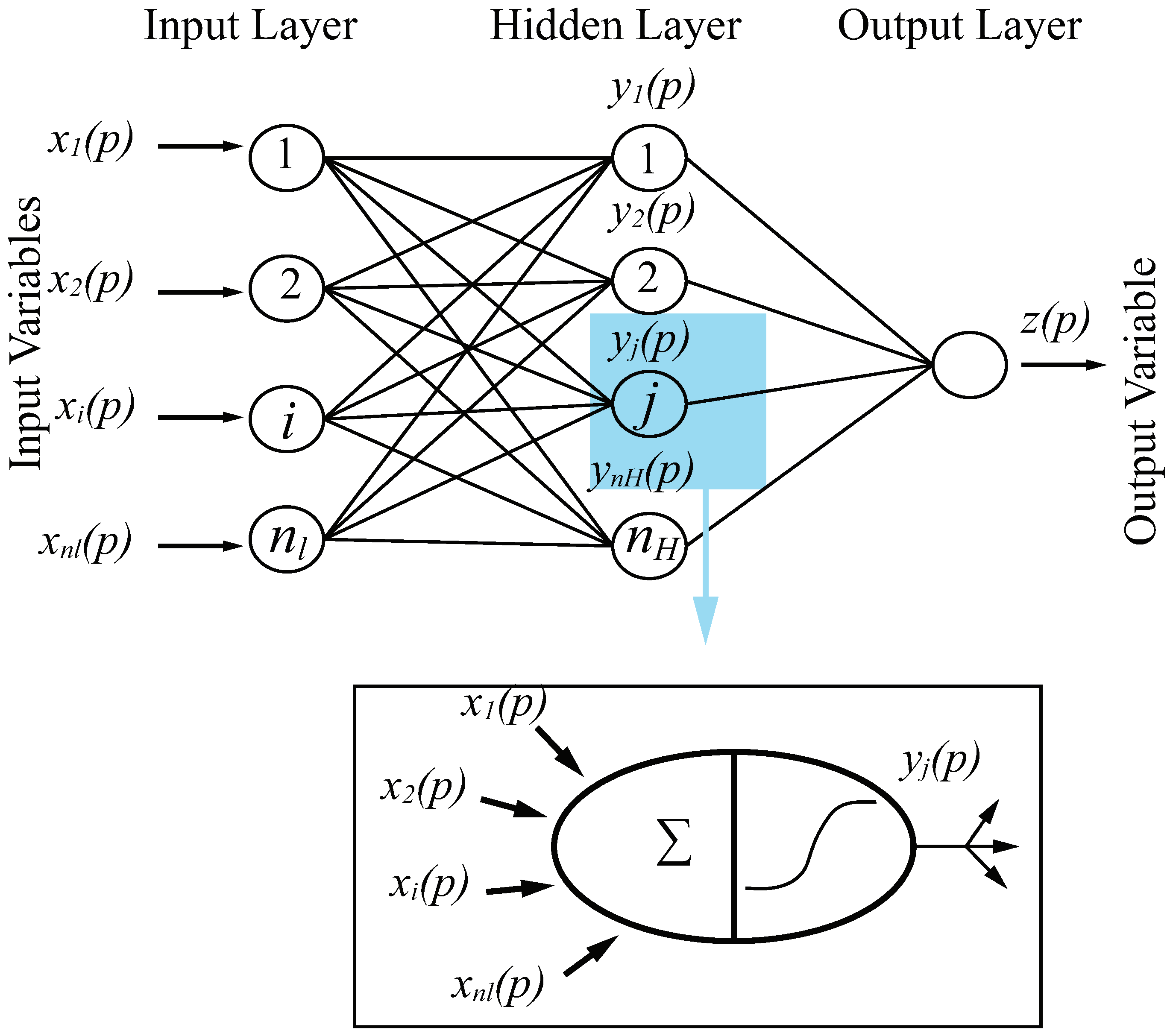
The ANN functions are similar to the human brain and nervous system which are a form of AI. ANNs can be trained with datasets to conduct prediction models and learn the intrinsic relationships without parameters [22]. These ANN models are being used as an efficient tool to reveal nonlinear relationship between inputs and outputs. Unlike conceptual models, using ANN models only dealing with mathematical relationship between inputs and outputs which are not defined. The commonly used ANN model (feed forward neural network) comprises of three layers of input, hidden and output (Figure 1). Each layer possesses a set of nodes (neurons) in which they are fully connected with nodes in the following layer. The model has a feed forward phase in which inputs signals propagate in forward direction (layer by layer) to reach output layer and an error backward propagation process which modifies the connection strengths (weights). Error is defined as the difference between computed and observed values of the target variable. Generally, the ANN model can be mathematically formulated as:

$$O_k=g_2[\sum _{j=1}^M{W}_{kj}{g}_1(\sum _{i=1}^N{W}_{ji}{x}_i+W_{jo})+W_{ko}]$$

(1)

where $x_i$ is the input value to node i, $O_k$ is the output at node k, $g_1$ is activation function (nonlinear) for the hidden layer and $g_2$ is activation function (linear) for the output layer. N and M represent the number of neurons in the input and hidden layers, respectively. $W_{jo}$ and $W_{ko}$ are biases of the jth neuron in the hidden layer and the kth neuron in the output layer. $W_{ji}$ is the weight between the input node i and the hidden node j, and $W_{kj}$ the weight between the hidden node j and the output node k.

2.2. RNN

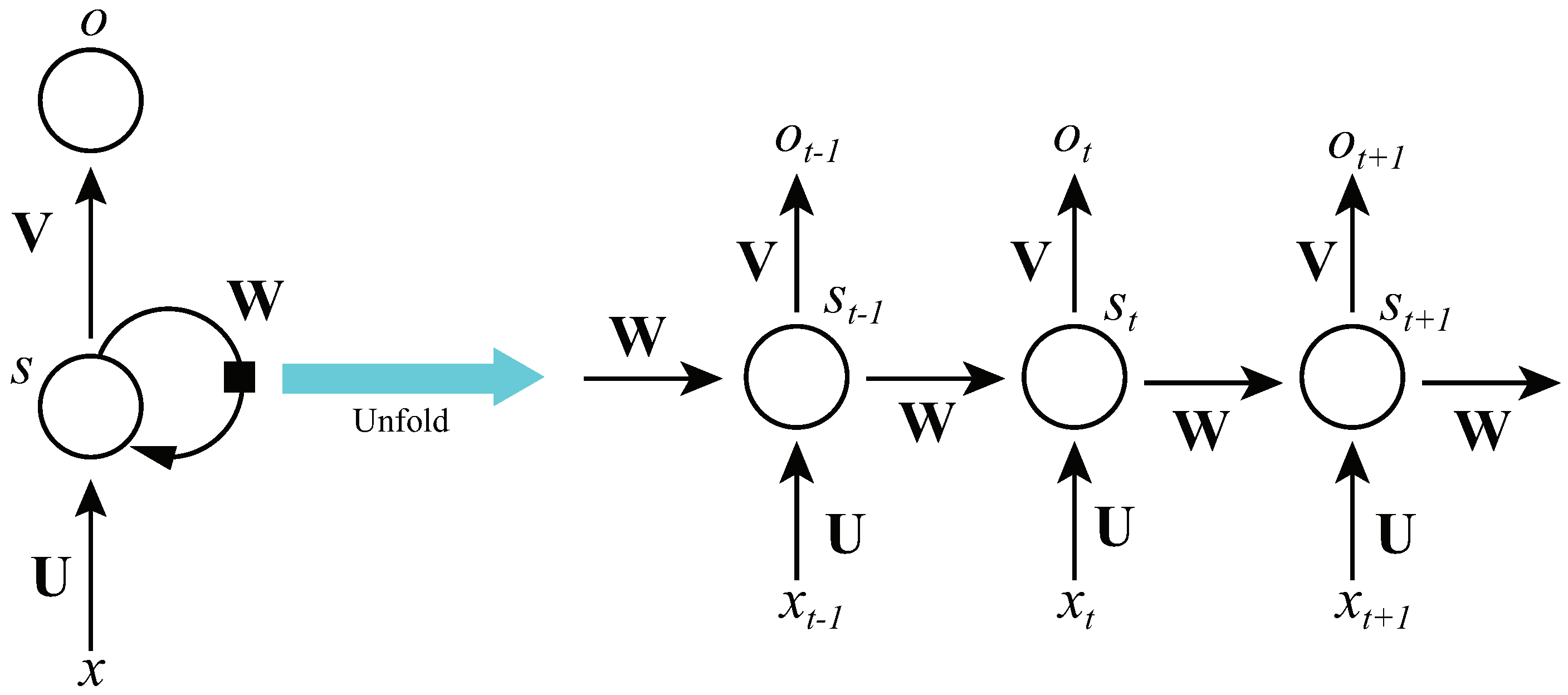
Recurrent neural networks (RNNs) are powerful model for sequential data. Recurrent neural network are a strict superset of feedforward neural networks, augmented by the inclusion of recurrent edges that span adjacent time steps, introducing a notion of time to the model [19]. While RNNs may not contain cycles among the conventional edges, recurrent edges may form cycles, including self-connections. At time t, nodes receiving input along recurrent edges receive input activation from the current example $x^t$ and also from hidden nodes $h^{t-1}$ in the network’s previous state. The output ${\widehat{y}}^t$ is calculated given the hidden state $h^t$ at that time step. Thus, input $x^{t-1}$ at time $t-1$ can influence the output ${\widehat{y}}^t$ at time t by way of these recurrent connections (Figure 2).

We can show in two equations that all calculations are necessary for computation at each time step on the forward pass in a simple recurrent neural network:

$$h^{(t)}=\sigma (W_{hx}x+W_{hh}{h}^{(t-1)}+b_h)$$

(2)

$${\widehat{y}}^{(t)}=softmax(W_{gh}{h}^{(t)}+b_y)$$

(3)

where $W_{hx}$ is the matrix of weights between the input and hidden layers and $W_{hh}$ is the matrix of recurrent weights between the hidden layers at adjacent time steps. The vectors $b_h$ and $b_y$ are biases which allow each node to learn an offset.

2.3. LSTM

LSTM networks belong to the class of recurrent neural networks (RNNs), i.e., neural networks whose “underlying topology of inter-neuronal connections contains at least on cycle”. They have been introduced by Hochreiter and Schmidhuber [24] and were further refined in the following years. LSTM networks are specifically designed to learn long-term dependencies and are capable of overcoming the previously inherent problems of RNNs, i.e., vanishing and exploding gradients (Figure 3).

LSTM networks are composed of an input layer, one or more memory cells, and an output layer. The number of neurons in the input layer is equal to the number of explanatory variables. The main characteristic of LSTM networks is contained in the hidden layer consisting of so called memory cells. Each of the memory cells has three gates maintaining and adjusting its cell state $s_t$: a forget gate $(f_t)$, an input gate $(i_t)$, and an output gate $(o_t)$.

At every time-step t, each of the three gates is presented with the input $x_t$ (one element of the ) as well as the output $h_{t-1}$ of the memory cells at the previous time-step $t-1$. Hereby, the gates act as filters, each fulfilling a different purpose:

• The forget gate defines what information is removed from the cell state.
• The input gate specifies what information is added to the cell state.
• The output gate specifies what information from the cell state is used

The sequential update formula are

• Input node

  $$g^{(t)}=tanh(W_{gx}{x}^{(t)}+W_{gh}{h}^{(t-1)}+b_g)$$

  (4)
• Input gate

  $$i^{(t)}=\sigma (W_{ix}{x}^{(t)}+W_{ih}{h}^{(t-1)}+b_i)$$

  (5)
• Forget gate

  $$f^{(t)}=\sigma (W_{fx}{x}^{(t)}+W_{fh}{h}^{(t-1)}+b_f)$$

  (6)
• Output gate

  $$o^{(t)}=\sigma (W_{ox}{x}^{(t)}+W_{oh}{h}^{(t-1)}+b_o)$$

  (7)
• Cell state

  $$s^{(t)}=g^{(t)}\odot i^{(t)}+s^{(t-1)}\odot o^{(t)}$$

  (8)
• Hidden gate

  $$h^{(t)}=tanh(s^{(t)})\odot o^{(t)}$$

  (9)
• Output layer

  $$y^{(t)}=(W_{hy}{h}^{(t)}+b_y)$$

  (10)

  where $\sigma$ is the sigmoidal function, ⊙ is element wise multiplication, $x^{(t)}$ is the input vector (forcings and static attributes) for the time step t, $W_s$ are the network weights, $bs$ are bias parameters, y is the output to be compared to observations, h is the hidden state, and s is called the cell state of memory cells, which is unique to LSTM.

2.4. Performance Evalution Criteria

In this study, performance of different models is assessed by statistical error measures and characteristic of flood process error including the coefficient of determination ($R^2$), root mean square error ($RMSE$), Nash-Sutcliffe Efficiency ($NSE$), mean absolute error ($MAE$), error of time to peak discharge ($E{T}_p$) and error of peak discharge ($E{Q}_p$).

$$R^2=\frac{{({\sum }_{i=1}^n(y_i-\overline{y})(y_i^{\prime }-{\overline{y}}^{\prime }))}^2}{{\sum }_{i=1}^n{(y_i-\overline{y})}^2{\sum }_{i=1}^n{(y_i^{\prime }-{\overline{y}}^{\prime })}^2}$$

(11)

where $y_i^{\prime }$ (m${}^3$/s) and $y_i$ (m${}^3/$s) represent the discharge of the simulated and observed hydrographs at the time i, $\overline{y}$ (m${}^3/$s) and ${\overline{y}}^{\prime }$ (m${}^3$/s) denote the average observed and simulated discharge at the time i and n is the data points number. The coefficient of determination, $R^2$, known as the square of the sample correlation coefficient, ranges from 0 to 1 and describes the amount of observed variance explained by the model. A value of 0 implies no correlation, while a value of 1 suggests that the model can explain all of the observed variance.

$$RMSE=\sqrt{\frac{{\sum }_{i=1}^n{(y_i-y_i^{\prime })}^2}{n}}$$

(12)

The root mean square error, $RMSE$, evaluates how closely that predictions match to observations, Values may range from 0 (perfect fit) to $+\infty$ (no fit) based on the relative range of the data.

$$NSE=1-\frac{{\sum }_{i=1}^n{(y_i-y_i^{\prime })}^2}{{\sum }_{i=1}^n{(y_i-\overline{y})}^2}$$

(13)

The Nash-Sutcliffe Efficiency, $NSE$, measures the model’s ability to predict variables different from the mean and gives the proportion of the initial variance accounted for by the model. Where $NSE$ ranges from 1 (prefect fit) to $-\infty$. Values less than zero indicate that the observation mean would be a better predictor than the model.

$$MAE=\frac{{\sum }_{i=1}^n|y_i^{\prime }-y_i|}{n}$$

(14)

The mean absolute error, $MAE$, measures the difference between observed and modelled results. It is an average of the absolute errors, where $y_i^{\prime }$ is the simulation and $y_i$ is the observation.

$$E{T}_p=|T_{m,p}-T_{o,p}|$$

(15)

The error of time to peak discharge, $E{T}_p$, measures the model’s time accuracy of peak runoff discharge prediction. Where $T_{m,p}$ (hour) and $T_{o,p}$ (hour) are the peak time for the modelled and observed peak runoff discharge, respectively.

$$E{Q}_p=\frac{(y_{m,p}-y_{o,p})}{y_{o,p}}\times 100\%$$

(16)

The error of peak discharge, $E{Q}_p$, measures the model volume accuracy of peak runoff discharge prediction. Where $y_{m,p}$ (m${}^3$/s) and $y_{o,p}$ (m${}^3$/s) are the modelled and observed peak runoff discharges, respectively.

2.5. The Approach and Modelling Process

In this study, data preparation and handing is entirely conducted in Python 3.5, relying on the packages numpy and pandas. Our LSTM and ANN networks are developed with keras on top of Google TensorFlow, a powerful library for large-scale machine learning on heterogenous systems.

We define the LSTM with 50 neurons in the first hidden layer and 1 neuron in the out layer for predicting discharge. The input shape will be 1 time step with 16 features. We will use the Mean Absolute Error (MAE) loss function and the efficient Adam version of stochastic gradient descent [25].

The type of ANN used in this study is a multi-layer-feed-forward perceptron (MLP) trained with the use of back propagation learning algorithm. The MLP network consists of input layer, hidden layer, and output layer. The final connection weights are kept fixed at the completion of training and new input patterns are presented to the network to produce the corresponding output consistent with the internal representation of the input/output mapping. In this study, the Levenberg–Marquardt (LM) algorithm is used for training the MLP network. The LM algorithm is often the fastest back propagation algorithm, and has been highly recommended as a first-choice supervised algorithm, although it does require more memory than other algorithms. Further information on the back propagation learning algorithms can also be found in Dawson [26].

The simulation function of discharge is shown as:

$$Q_t=f(Q_{t-n},R_{t-n},X_{t-n})$$

(17)

in which $Q_t$ is current flow, $Q_{t-n}$ is antecedent flow (at $t-1, t-2, \dots , t-n$ time steps), $R_{t-n}$ is antecedent rainfall (at $t-1, t-2, \dots , t-n$), and $X_{t-n}$ represents any other factors identified as affecting $Q_t$ (e.g., year type, percentage impervious area, storm occurrence). In this paper, we used the 14 rainfall stations and antecedent flow to forecast the runoff. We have chosen different values of n with 1, 2, 3, 4, 5, 6 (hour) indicating 6 types of lead time.

3. Case-Study

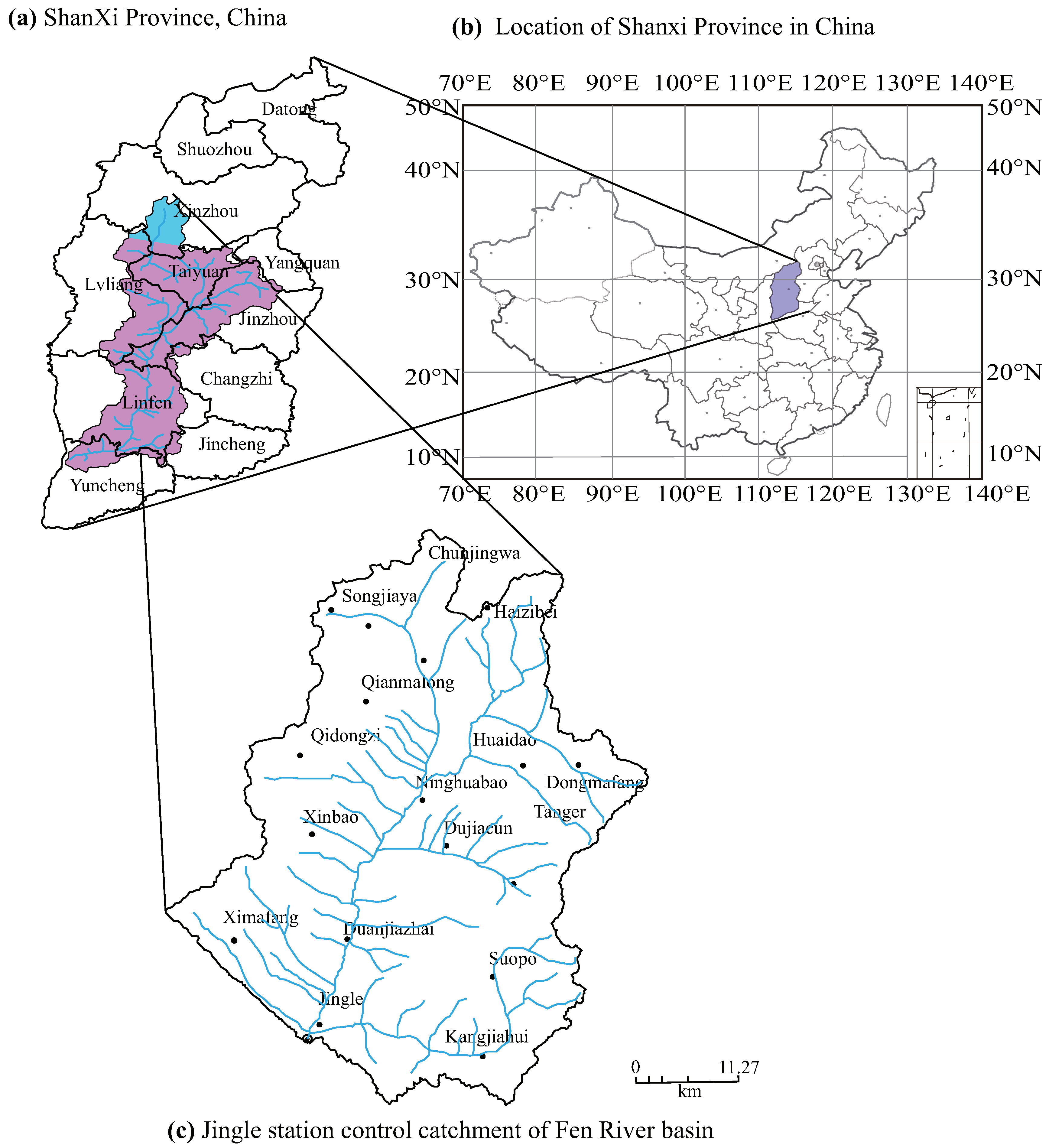
Fen River Basin (${35}^{\circ }{20}^{\prime }$–${39}^{\circ }{00}^{\prime }$ N latitude, ${110}^{\circ }{30}^{\prime }$–${113}^{\circ }{32}^{\prime }$ E longitude) is located in Shanxi Province, North China (Figure 4). The Fen River is one of the largest tributaries of the Yellow River in its middle reach, joining the Yellow River in Hejing County. The river basin is bounded by Taihang Mountain to the east, and Lvliang Mountain to the west, which also form the boundary between Yellow River and Fen River. Located in the eastern Loess Plateau of China, the climate of the Fen River Basin is temperate and sub-humid, with mean annual precipitation of 450 mm. In this area, the landforms are usually capped by a thick layer of loess due to dust deposition during the Quaternary. The study region is the catchment of Jingle hydrology station. The Jingle station was constructed in April on 1943 which was control station in main upstream of Fen River. The area of Jingle station controled basin is 2799 km${}^2$ and the length of main stream is 83.9 km with average slope 0.67%. There are four tributaries in this basin, namely Hong river, Mingcun river, Dongnian river and Xinian river.

The annual mean precipitation in Jingle control basin is about 538.38 mm, the amount of mean flood in 24 h is about 50–55 mm, the maximum rainfall in the single site over 24 h is 109.6 mm. The average peak runoff and maximum peak runoff is 594 and 2230 m${}^3/$s. The rainfall station is shown by Figure 4c. The downstream Jingle discharge station is the forecasting object. This study collected hourly discharge data from Jingle station and hourly rainfall data from fourteen gauges. Data for 98 flood events from 1971 to 2013 with complete records were obtained. Among these flood events, 82 events (4962 datasets) were used for calibration and 12 events (1488 datasets) were used for validation red In this paper, we have chosen the typical rainfall-runoff process for validation to make the network models more representative, namely, the big volume discharge, the normal volume discharge in different periods from 1971 to 2013.

4. Results

Every flood event is so different with rainfall duration, peak discharge, rainfall center (

Table 1. Characteristics of collected flood events in Jingle discharge station.

Event No.	Date	Total Rainfall (mm)	Rainfall Duration (h)	Rainfall Center	Peak Discharge (m${}^3$/s)
1	1 July 1971	8.86	36	Ninghuabao	164.50
2	23 July 1971	63.40	69	Chunjingwa	261.21
3	31 July 1971	10.44	12	Dongzhai	286.00
4	7 August 1971	21.07	42	Ninghuabao	184.14
5	15 August 1971	7.60	16	Chunjingwa	145.00
6	27 August 1971	15.71	36	Chunjingwa	112.00
7	31 July 1972	11.98	15	Huaidao	142.43
	...	...	...	...	...
92	10 October 2007	43.88	57	Chashang	106.00
93	23 September 2008	70.49	88	Qidongzi	132.00
94	10 August 2010	70.50	24	Songjiaya	67.00
95	11 July 2011	41.88	24	Dujiacun	54.35
96	26 July 2012	40.57	41	Ninghuabao	134.00
97	30 July 2012	41.95	41	Chashang	61.90
98	17 July 2013	29.91	32	Jingle	74.40

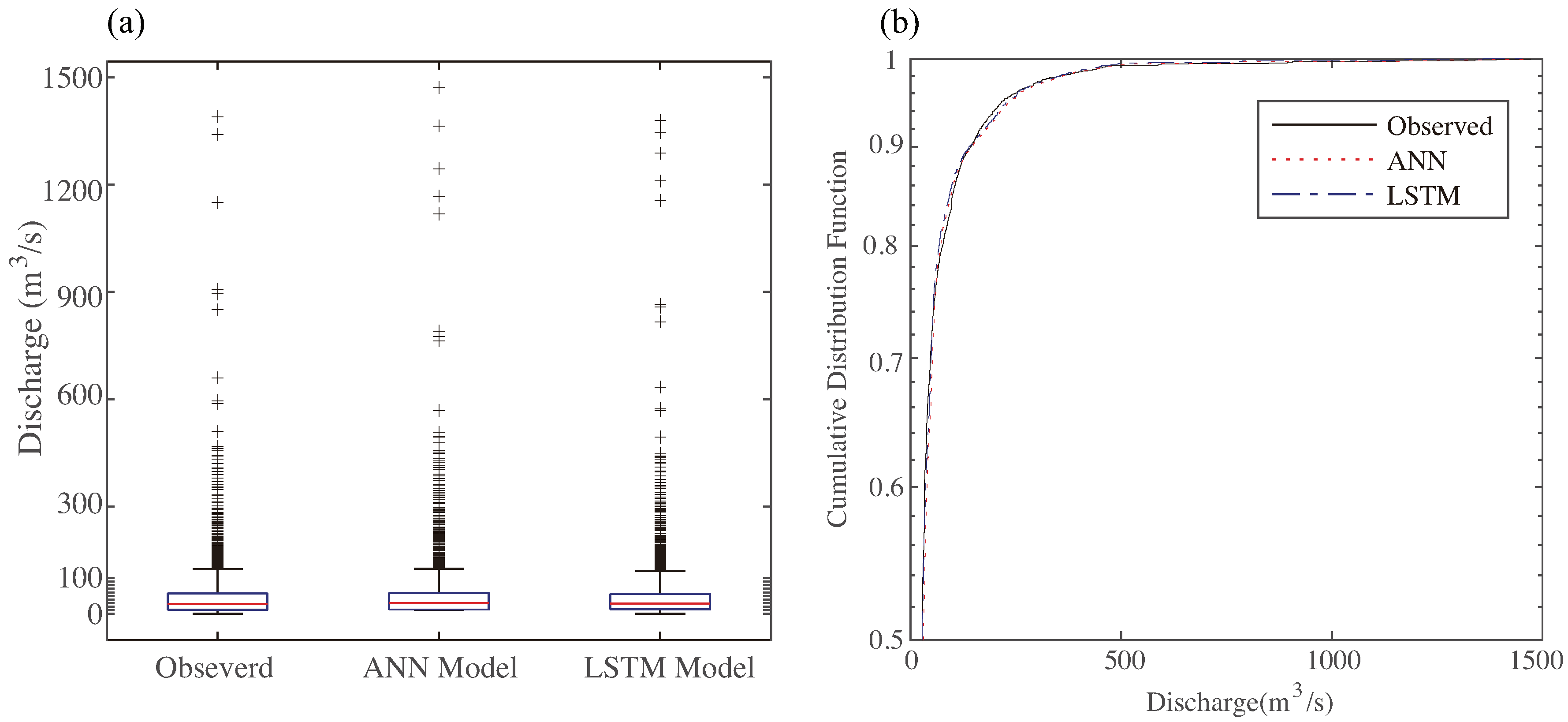
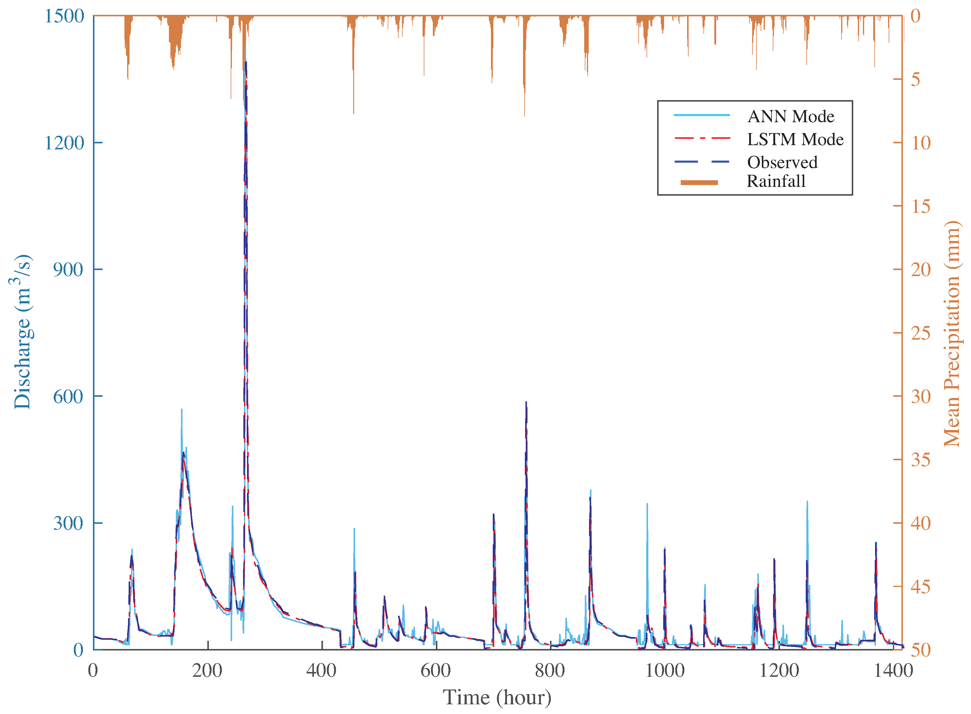
) that the process rainfall-runoff is difficult to learn. The Figure 5 illustrates that the statistical characteristics of 12 flood events data for validation. The upper boundary of Figure 5 is not above 150 (m${}^3$/s). The rapid flooding with large volume discharge in a short time makes many outliers in the dataset, but this typical large flooding is not common only 6 events (6.1%) (peak discharge above 1000 (m${}^3$/s)) over the period from 1971 to 2013. Thus, we also seriously considered the sudden bigger data in constructing models. From Figure 5a, ANN model made some bigger forecasting values comparing with observed data when discharge data was exceeded 1200 (m${}^3$/s). While the LSTM model is better than ANN model at the same situation. The Figure 5b is shown the cumulative distribution of observed and modelled data. The three Lines almost coincided indicating that ANN and LSTM models have similar forecasting preferences in low volume discharge simulation. It also illustrates that the value of discharge among 0–200 (m${}^3$/s) takes percentage of almost 90%. From the analysis of dataset characteristics, we could find it is difficult for rainfall-runoff simulation taking into account sudden big and small volume of discharge. However, the above results lead to preliminary conclusion that ANN and LSTM models have better performances in flooding forecasting.

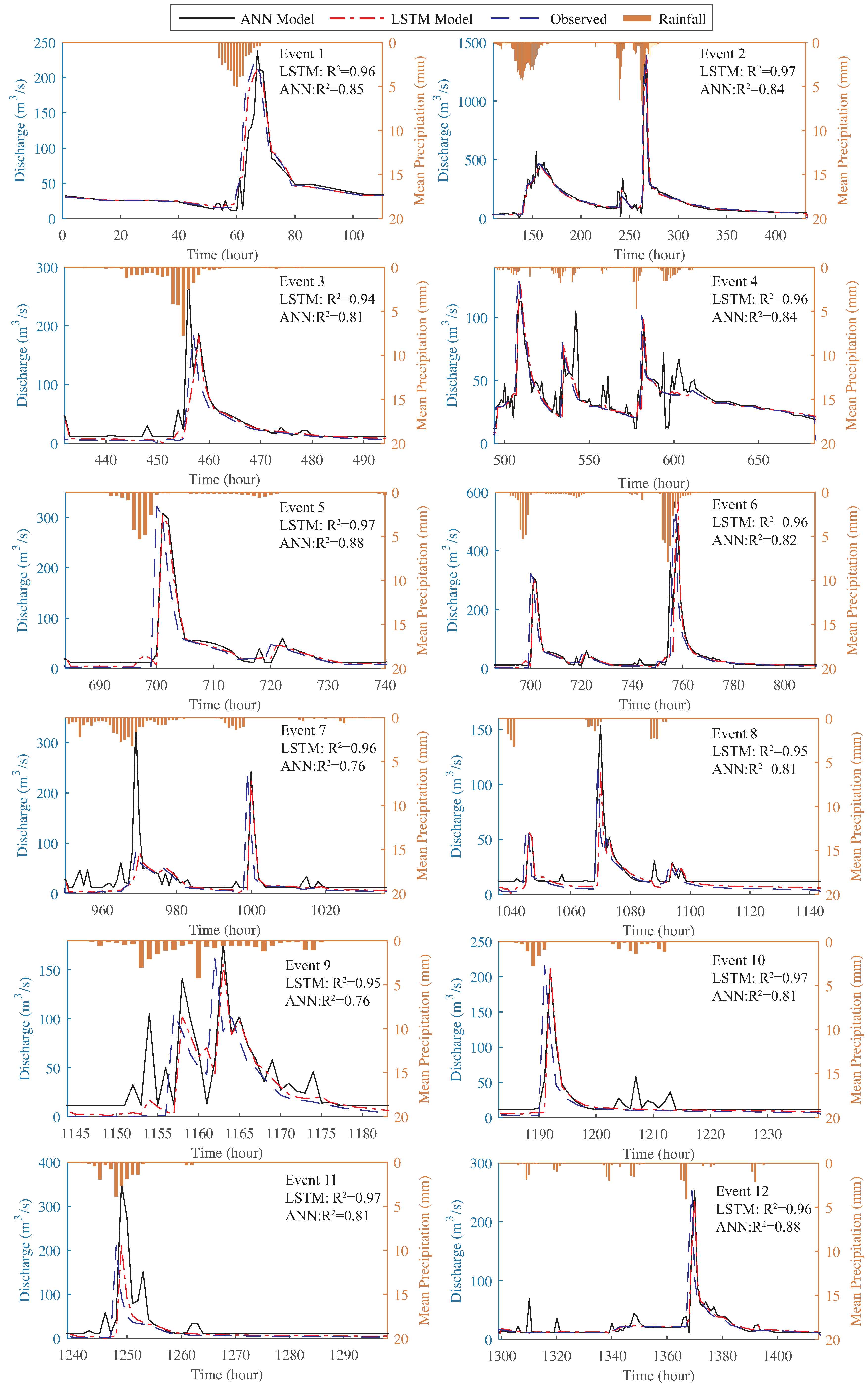
In the above study, we discussed statistical features of validation data. Then, the estimated hydrograph was used to compare performance of different models in validation (Figure 6). Even though the flooding process is difficult for simulation, the ANN and LSTM models all simulated well in general. Comparing with the peak discharge simulation, the value of ANN modelled were always bigger than observed data. In the low value of discharge simulation, the ANN modeled values appeared abnormal fluctuations. From estimated hydrograph Figure 6, it shows that LSTM model is more stable and simulated very well than ANN model. Thus, the LSTM model has better ability in nonlinearity simulation.

Table 2. Comparison of performances of ANN and LSTM models for runoff prediction (lead time = 1 h) at calibration (86 flood events) and validation (12 flood events) periods.

Events	Modes	${\mathit{R}}^2$	$\mathit{RMSE}$ (m${}^3$ s${}^{-1}$)	$\mathit{NSE}$	$\mathit{MAE}($m${}^3$ s${}^{-1}$)	${\mathit{ET}}_{\mathit{p}}$ (h)	${\mathit{EQ}}_{\mathit{p}}$
Calibration
86 events series	ANN	0.81	124.21	0.83	47.23	5.4	12%
	LSTM	0.95	45.12	0.97	12.4	2.6	4%
Validation
12 events series	ANN	0.83	35.6	0.83	23.6	3.7	14%
	LSTM	0.96	12.4	0.96	6.3	1.4	3%

makes comparison of performances of ANN and LSTM models for runoff prediction. This is quantitative analysis of ANN and LSTM models using 6 preference criteria. The values of $R^2$ and $NSE$ are all beyond 0.95 in the LSTM modelling results in calibration and validation periods. Comparing with ANN model, the LSTM model values of $RMSE$, $MAE$, $E{T}_p$ and $E{Q}_p$ are all less than ANN indicating better performances in rainfall-runoff simulation. Especially, the ANN values of $E{Q}_p$ are almost 4 times bigger than LSTM model. These cases illustrate that the LSTM model have accurately simulated peak discharge. The prediction of peak discharge of flood is critical for hydrological process simulation. Thus, the new model of LSTM with complicated architecture is a good choice for rainfall-runoff simulation and flood forecasting.

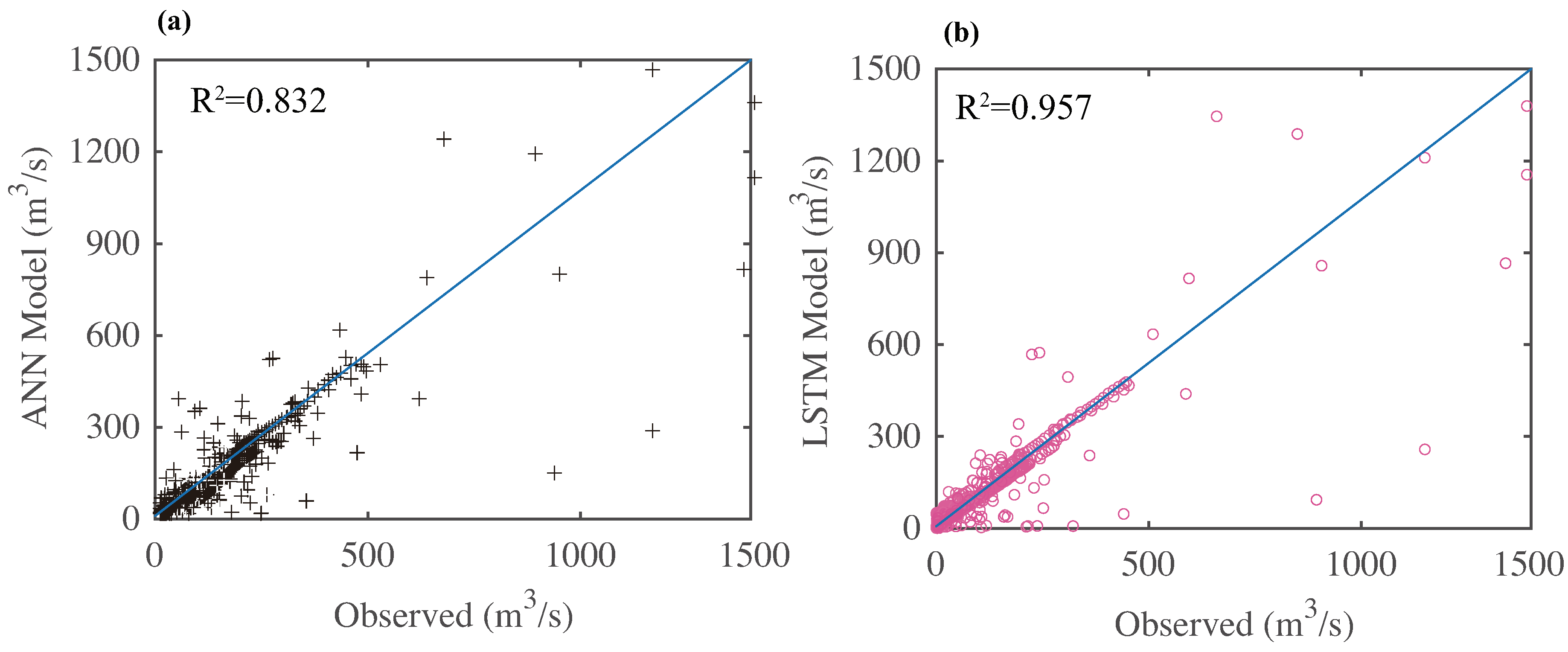
After quantitative and qualitative analysis of ANN and LSTM models, we also scatter the observed and simulated discharge values (Figure 7). The values of ANN and LSTM models’ $R^2$ are 0.832 and 0.957, respectively. The LSTM model has higher values of $R^2$ indicating that this model could well reflect the relationship between observed and simulated discharge. From the Figure 7a, the data is scattered more loose in ANN model, while it is relatively closer to the line in LSTM model (Figure 7b). It is clearly shown that LSTM model is better than ANN model in runoff prediction which has better correlation with observed data. Besides, the values are almost near the fit line in the two models. However, the two models all appear some abnormal values. The reason of this phenomenon is that ANN and LSTM models have some fluctuations under the suddenly changes in rainfall and discharge data.

We have talked about general characteristics of ANN and LSTM models in above study. However, some special features need to deeply insight into ANN and LSTM models for hydrological process simulation. The Figure 8 shows observed and estimated hydrographs of the ANN and LSTM models at the validation stage in 12 flood events. Among the 12 flooding events, only peak discharge of event 2 was beyond 1000 (m${}^s$/s). The ANN model has bed ability of peak discharge prediction comparing with LSTM model. In the flooding event 1, 3, 4, 8, 9, and 11, the simulated peak discharge always higher than observed. These modelled values of peak discharge were not to be trusted in flooding event 7, 8 and 11 with abnormally bigger values. However, the LSTM model was proved more reliable in prediction of peak discharge. We can take flooding event 4, 7, 9 and 10 that ANN model always has much sensitivity to rainfall. The simulated values of ANN model fluctuate abnormally comparing with observed values no matter big or small volume discharge. While the LSTM model don’t appear these performances. The differences in ANN and LSTM model architectures are memory cells. The various memory cells have ability to filter data and memory data features making as deep learning function to simulate rainfall-runoff process. The disadvantages of ANN model are obvious. Compared with ANN and LSTM models in these flooding event simulation, it is proved that LSTM model is more intelligence than ANN model in predicting rainfall-runoff.

We have already discussed ANN and LSTM models simulation performances using lead time 1 h in above. The

Table 3. The performances of runoff forecasting at different lead times (1–6 h) by ANN and LSTM model for series flood events.

Lead Time (h)	Data	Models	${\mathit{R}}^2$	$\mathit{RMSE}$ (m${}^3$ s${}^{-1}$)	$\mathit{NSE}$	$\mathit{MAE}$ (m${}^3$ s${}^{-1}$)	${\mathit{ET}}_{\mathit{p}}$ (h)	${\mathit{EQ}}_{\mathit{p}}$
1	Calibration	ANN	0.81	124.21	0.83	47.23	5.4	12%
		LSTM	0.95	45.12	0.97	12.4	2.6	4%
	Validation	ANN	0.83	35.6	0.83	23.6	3.7	14%
		LSTM	0.96	12.4	0.96	6.3	1.4	3%
2	Calibration	ANN	0.83	132.2	0.86	42.13	11.4	13%
		LSTM	0.95	42.12	0.94	13.4	2.4	7%
	Validation	ANN	0.79	23.6	0.85	23.1	2.7	12%
		LSTM	0.93	15.4	0.95	6.3	1.8	13%
3	Calibration	ANN	0.78	164.21	0.79	56.23	14.4	11%
		LSTM	0.91	47.12	0.91	13.4	2.8	6%
	Validation	ANN	0.81	25.6	0.78	23.6	4.2	15%
		LSTM	0.92	14.4	0.91	7.3	1.4	16%
4	Calibration	ANN	0.81	144.21	0.82	48.23	11.4	12%
		LSTM	0.91	65.12	0.91	15.4	2.8	12%
	Validation	ANN	0.72	37.8	0.81	25.6	3.1	11%
		LSTM	0.91	13.4	0.93	11.3	1.6	15%
5	Calibration	ANN	0.78	135.21	0.81	48.23	11.4	12%
		LSTM	0.87	49.12	0.81	17.4	4.6	8%
	Validation	ANN	0.74	38.6	0.79	24.6	5.7	16%
		LSTM	0.84	22.4	0.91	6.3	1.4	17%
6	Calibration	ANN	0.71	144.21	0.73	67.23	18.4	17%
		LSTM	0.84	48.12	0.96	13.4	2.7	12%
	Validation	ANN	0.75	25.6	0.79	23.6	3.7	14%
		LSTM	0.83	14.4	0.85	8.3	2.4	18%

illustrates runoff forecasting at different lead times (1–6 h) by ANN and LSTM model. In general, LSTM model had better simulation results than ANN model at different lead times. In the calibration and validation stage, the values of performances criteria in LSTM model are all better than ANN models. Comparing with different lead time situations, the values of $R^2$ and $NSE$ were reducing with the increasing lead time. The values of $RMSE$, $MAE$ and $E{T}_p$ did not show clearly changing law. The LSTM values of $E{Q}_p$ was the smallest in lead time at 1 h. While the ANN model had badly performances in lead time at 6 h as the values of $R^2$ and $NSE$ near 0.7. Even though LSTM prediction ability was inducing with large lead time, the values of $R^2$ and $NSE$ still above 0.8. Compared with the ANN model, LSTM also has the low value of $E{T}_p$ and $E{Q}_p$. These results illustrate that the LSTM has the better performances in forecasting peak discharge in each flood event. These results mean that the chosen of LSTM model is suitable for the rainfall-runoff modeling. From all of these results, we can considerer LSTM network suitable using in hydrology research.

5. Discussion and Conclusions

The process of rainfall-runoff simulation is critical for hydrology [27]. However, the process of rainfall-runoff is a complex problem for the hydrological modelling. Saturated and infiltration excess runoff could all appear in one rainfall-runoff event in semi-dry and semi-humid region. Conducting suitable models is more complicated into semi-dry and semi-humid regions. The mechanism of runoff generation is more complicated than humid region. Considering the features of climate and hydrological process, lots of watershed belong to semi-dry and semi-humid region in China. Thus, the performances of physical models and conceptual models were badly used that the correlation coefficients were around 0.6 in this semi-dry and semi-humid regions [28,29]. However, in a recently study of rainfall-runoff simulation, various artificial networks were used for the simulation and prediction [30]. In this study, we use the traditional network as ANN and the new deep learning network as LSTM for the simulation. In generally, LSTM model is better than the traditional ANN model. Because of the typical flood characteristics, the ANN models can not make accurate simulation [31], but the ANN models are still better than the physical models in this region. It is the progress of the AI based techniques making the revolutionary strides for hydrology [4].

Compared with other network models, Kan [31] used a hybrid data-driven (network model and physical model) models for event-based rainfall-runoff simulation. PEK model (hybrid model) outperformed other models with values of $NSE$ and $R^2$ are 0.51 and 0.73, respectively in validation stage. However, the results of this study all better than Kan’s. There are two factors as inputs and model architecture that affect results of model outputs. In this paper, we used 14 rainfall stations data and antecedent discharge as the inputs. The dataset in this paper was larger than Kan’s. We used the network model with memory cells (LSTM) that was progressed than his model. Thus, we got the better simulation performances. Lin [30] forecasted the typhoon-rainfall with a hybrid neural network model (the Self-Organizing Map (SOM) and Multilayer Perceptron Network (MLPN)). In Lin’s study, SOM network was used for classification rainfall and then the MLPN was used for prediction. This model can forecast more precisely than the model developed by the conventional neural approaches, but the values of $NSE$ were below 0.85. These values were also smaller than LSTM modeling results in this study. The reason was that LSTM model with memory cells could learn more from the datasets and accurately make simulation.

However, the hydrological cycle process significantly changed under human activities and climate changes in Loess Plateau where have implemented project of returning farmland to forest and protecting natural forecast from 1980s. The changeable environments also make influence on rainfall-runoff process [32]. It is important to test if the LSTM or ANN model could be used in this region. Compared with simulated 12 flooding events (lead time 1 h Figure 8), the values of correlation efficient were beyond 0.95 indicating that LSTM model was adaptable among different situations. Besides, the ANN model had bad adaptability with many abnormal simulations in changeable environment. In this study, LSTM model still had better performance when lead time was 6 h. Thus, LSTM could be used in this region for flooding prediction.

Compared with the previous study in rainfall-runoff modeling, the results of LSTM modeling have the higher values of $R^2$ and $NSE$. The LSTM model had perfect performances in this paper, while it needed to be validated in numerous watersheds. Thus, the more and more studies need to study deep learning model (LSTM) application in hydrology. And finding the meaning of intrinsic structure parameters of LSTM can also improve our learning of hydrology process. Then, the AI techniques may accurately be applied in hydrology.

In this research, we used ANN and LSTM models for forecasting hourly runoff discharges in Jingle hydrology station control catchment basin. Comparing with conceptual and physical-based models, these black box models can well simulate rainfall-runoff process with excellent performance evaluation criteria. Compared with flooding events simulation, ANN model is more sensitive that has many abnormal fluctuations, while LSTM model is more intelligence than ANN model. In this study, the runoff is changed in time-series that the data is time related. The ANN model is constructed by fitting the different characteristics of the current state and making prediction. While LSTM model not only take full advantage of the current data characteristics but also use its gate structure to decide to remember or forget the previous features. With the progress of AI techniques, the deep learning methods of long short-term memory network could be better used in the hydrological simulation. The values of $R^2$ and $NSE$ in LSTM model are bigger than 0.9 when lead time is 1 h. With increment of lead time, values of performance criteria ($R^2$ and $NSE$) were slightly decreasing, but the values of LSTM model were still beyond 0.8 with good simulation abilities. It is because of LSTM is very effective in modeling time-series data, it can also be applied to weather forecasting, for example rainfall, fog and haze, stream flow et al. In this paper, we considered the data of the preceding hours to predict the runoff of the next hours. In the future, we could forecast different length of time or not only runoff forecasting, we can predict the entire sequence of data at the next moment. This deep learning networks have better performances in hydrological time-series prediction. More researches will be needed in modelling hydrological process using deep machine learning.