Article

Infilling Missing Data in Hydrology: Solutions Using Satellite Radar Altimetry and Multiple Imputation for Data-Sparse Regions

by
Iguniwari Thomas Ekeu-wei
1,*,
George Alan Blackburn
1 and
Philip Pedruco
2
1
Lancaster Environment Centre, Lancaster University, Lancaster LA1 4YQ, UK
2
Jacobs Engineering Group Inc., Melbourne, VIC 8009, Australia
*
Author to whom correspondence should be addressed.
Water 2018, 10(10), 1483; https://doi.org/10.3390/w10101483
Submission received: 6 September 2018 / Revised: 5 October 2018 / Accepted: 10 October 2018 / Published: 20 October 2018
(This article belongs to the Special Issue Hydrologic Modelling for Water Resources and River Basin Management)

Abstract

:
In developing regions missing data are prevalent in historical hydrological datasets, owing to financial, institutional, operational and technical challenges. If not tackled, these data shortfalls result in uncertainty in flood frequency estimates and consequently flawed catchment management interventions that could exacerbate the impacts of floods. This study presents a comparative analysis of two approaches for infilling missing data in historical annual peak river discharge timeseries required for flood frequency estimation: (i) satellite radar altimetry (RA) and (ii) multiple imputation (MI). These techniques were applied at five gauging stations along the floodprone Niger and Benue rivers within the Niger River Basin. RA and MI enabled the infilling of missing data for conditions where altimetry virtual stations were available and unavailable, respectively. The impact of these approaches on derived flood estimates was assessed, and the return period of a previously unquantified devastating flood event in Nigeria in 2012 was ascertained. This study revealed that the use of RA resulted in reduced uncertainty when compared to MI for data infilling, especially for widely gapped timeseries (>3 years). The two techniques did not differ significantly for data sets with gaps of 1–3 years, hence, both RA and MI can be used interchangeably in such situations. The use of the original in situ data with gaps resulted in higher flood estimates when compared to datasets infilled using RA and MI, and this can be attributed to extrapolation uncertainty. The 2012 flood in Nigeria was quantified as a 1-in-100-year event at the Umaisha gauging station on the Benue River and a 1-in-50-year event at Baro on the Niger River. This suggests that the higher levels of flooding likely emanated from the Kiri and Lagdo dams in Nigeria and Cameroon, respectively, as previously speculated by the media and recent studies. This study demonstrates the potential of RA and MI for providing information to support flood management in developing regions where in situ data is sparse.

1. Introduction

As floods become increasingly more frequent, intense and devastating due to changing climatic conditions and anthropogenic factors [1], reliable hydrological information is required by flood risk managers and stakeholders alike to inform the deployment of interventions to mitigate flood impact [2]. Typically, networks of river gauging stations are established across several locations of interest to collect the necessary data over a given period [3]. However, operating such observatory systems—especially in developing regions—is often problematic due to financial (underfunding of data collection agencies), institutional (lack of technical capacity and commitment), operational (inaccessibility to remote gauge stations due to logistical and security challenges), and technical (equipment malfunction, replacement, damage, modification, discontinuity and manual data entry procedures prone to errors) factors [4,5,6].
These factors contribute to hydrological network inadequacy, the decline in functional stations, and gaps in available historical records, that consequently impact on the outcome of flood modelling processes required to inform decision making. Even when data is available, in many developing regions, these records are usually short, and manual river water level measurements and discharge estimation processes further subject the available hydrological data to aleatory and epistemic uncertainties [7].
Over the past decade, several approaches have been explored to compensate for data deficiencies to estimate flows for ungauged or sparsely gauged river basins, including remote sensing [8,9], hydrodynamic modelling [10], combined remote sensing and hydrodynamic models [11,12], catchment geomorphological and meteorological data integration [13], and hydrological regionalization [14], resulting in the estimation of river water levels and discharge with reduced levels of uncertainty. These techniques provide varying merits and demerits and are applicable in different scenarios, depending on available complementary data. Furthermore, these approaches require some form of ground data for verification, given that in situ observations provide better insight into local hydrological processes and catchment responses to changing climatic and landscape conditions [15], and the output of each technique is strongly dependent on the input data accuracy.
Irrespective of the method adapted for flood magnitude estimation, gaps within the hydrological time-series increase the uncertainty in flood estimates, resulting in flawed flood management decisions and interventions [16]. To curtail this deficiency, statistical and empirical methodologies have been widely deployed [17]. Statistical techniques focus on filling missing data by simulating trends/patterns within available datasets, using methods such as regression analysis [4,18], interpolation [19,20], and artificial neural networks [21].
Other traditional missing data infilling approaches generally involve the removal/deletion of gaps in existing data or application of single data imputation methods such as arithmetic mean or median imputation, regression, and principal component analysis [22]. Though the deletion method is usually convenient [23], this approach reduces sample size, thereby introducing statistical bias and reducing the statistical power and precision of standard statistical procedures [24]. Conversely, single imputation approaches replace missing data while retaining the original sample size. Nevertheless, single imputation techniques can lead to distorted parameter estimates, reduced data variability [24], predictable bias, high variable correlation [25] and dimensional subjectivity [26].
To curtail the limitations of single imputation approaches, multiple imputation (MI) has been proposed, an approach that replaces missing time series values using two or more plausible values derived from a distribution of possibilities [27]. MI is widely used in hydrological studies [27,28,29] and provides the unique advantages of accounting for missing data uncertainty and does not overestimate correlation error [30].
Empirical methods have also been applied to fill missing hydrological data, and usually require supplementary data from upstream or downstream gauging stations close to the location of interest, as well as other datasets such as digital elevation models [31]), bathymetry [32], satellite imagery [8,9,33] and radar altimetry [34]. Of all empirical approaches listed, only radar altimetry (RA) provides direct water level estimates that can be seamlessly integrated into existing hydrological time series without complex computation and models [35,36] that are rarely available nor applied in developing regions due to lack of capacity and high computational cost [37]. Also, given that altimetry virtual station networks are globally distributed [38], developing regions stand to benefit, especially in locations where manual observations are disrupted and measurement equipment destroyed by high magnitude flows during by peak flood seasons. Furthermore, the recent launch of Jason-3 [39] and Sentinel-3 [40] in early 2016, and the proposed Surface Water and Ocean Topography (SWOT) in 2020 [41] are expected to enhance continuous, long-term, and sustainable RA data collection. Notwithstanding, the applications of RA can be limited by factors including the state of atmosphere during data acquisition, satellite sensor properties, temporal resolution, water surface characteristics, and altimetry ground footprint, which can contribute to measurement variability and uncertainties [12,42].
In this context, the aim of this study was to identify and apply suitable techniques for resolving the problems of missing hydrological data which are common in developing regions. The objectives were to:
  • Determine the effectiveness of RA and MI approaches for filling missing data in hydrological timeseries.
  • Assess the impact of both approaches on flood frequency that is estimated given varying quantities of missing data.
  • Quantify the magnitude of the devastating 2012 flood in Nigeria (the study region for this research), after identifying the optimal infilling approach.
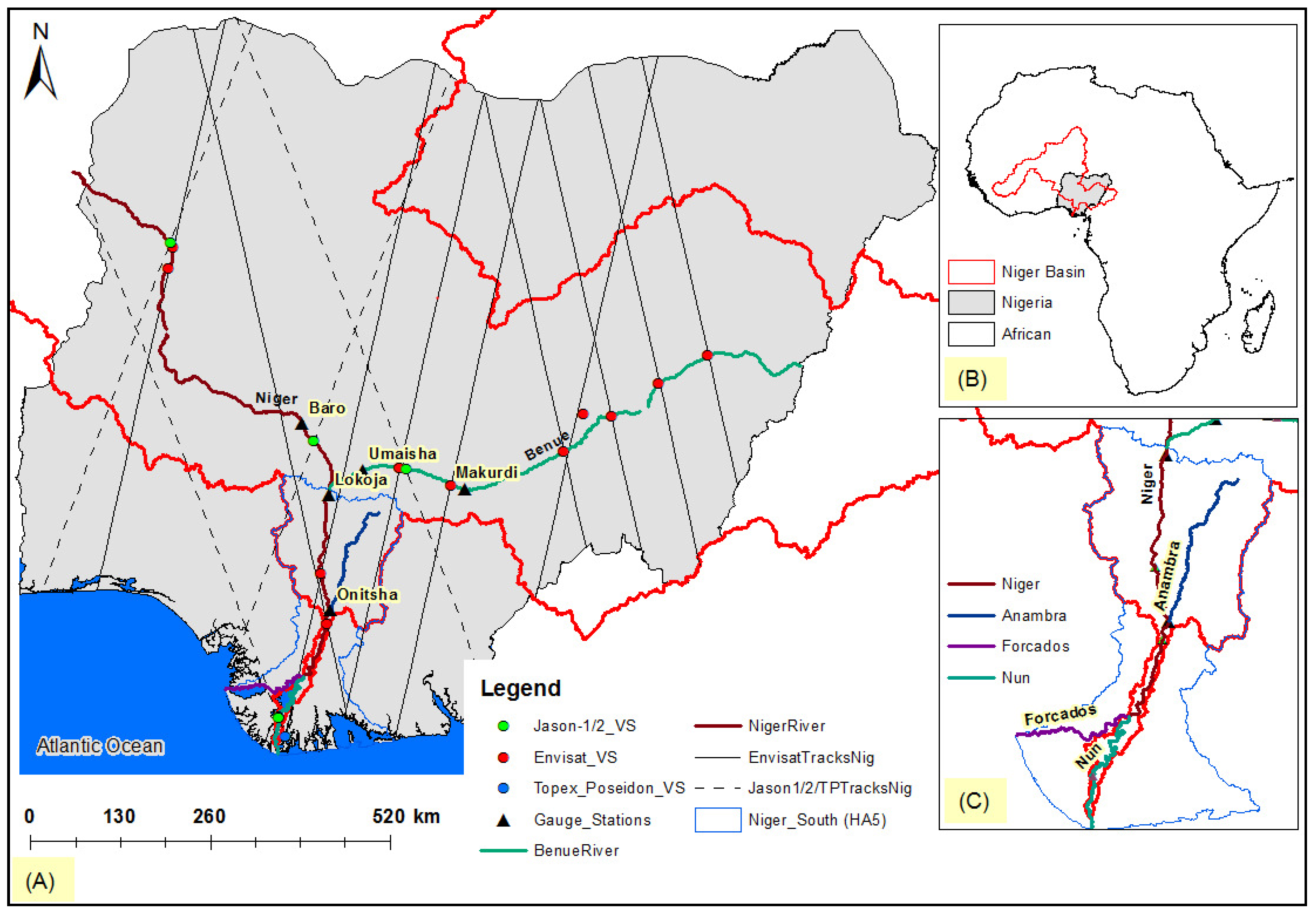
2. Study Region

The study region, the Niger-South Hydrological Area (HA) 5 (Figure 1A), encircles a population of 22,170,300 within a 54,000 km2 area. The hydrology of the region is defined by inflow from the Niger River Basin through Niger and Benue rivers (Figure 1B) travelling downstream to the Atlantic Ocean through the Nun and Forcados distributaries in the Niger Delta (Figure 1C), and to the Anambra-Imo river basin through the Anambra river. The annual rainfall varies from 1100 to 1400 mm, while the land cover along the Niger and Benue river floodplains is comprised of built-up areas (0.68%), cultivated land (31.42%), plantations (0.04%) wetlands (9.70%), mixed land use (36.85%), grasslands (6.17%), water bodies (14.83%), and bare surfaces (0.31%) [43]. The average annual discharge into the Niger-South river basin form the Niger and Benue river catchment areas is 5381 m3/s [44], and has an average river with of 742 m [10].
In 2012, the Nigerian states within HA-5 (i.e., Kogi, Anambra, Imo, Delta Bayelsa and Rivers) were heavily impacted during a flood event that resulted in the disruption of socio-economic activities, damage to properties and infrastructure and fatalities [45,46]. The 2012 flood event was reported to have caused the greatest impact/damage in 40 years [47,48] including: (i) economic and infrastructure loss worth 16.9 billion US Dollars, (ii) displacement of 3.8 million people, and (iii) loss of 363 lives [45]. This event was reportedly triggered by torrential rains which resulted in the release of excess water from dams in Nigeria (Kainji, Shiroro, and Kiri) and Cameroon (Lagdo), with the impact exacerbated by poor planning due to insufficient data availability and poor communication between Cameroon and Nigeria [45,47,49]. Recurring flooding is currently occurring in 2018, emanating from upstream water release from river Nigeria [50].
HA-5 faces the challenge of severe data sparsity and the availability of RA virtual stations along its constituent rivers (Niger and Benue) provides a valuable opportunity to curb this challenge, while MI presents an alternative approach for infilling missing hydrological data where RA is unavailable. Figure 1 shows in situ gauging stations in relation to radar altimetry tracks and virtual stations (Jason 1/2, Envisat and Topex/Poseidon) along the Niger and Benue rivers and Niger-South river basin.

3. Materials and Methods

3.1. In Situ Hydrological Data

The hydrological data (discharge, water levels, and rating curves) for the five in situ gauging stations (Table 1) were acquired from the Nigerian Hydrological Service Agency (NIHSA), National Inland Waterways Authority (NIWA) and Niger Basin Authority (NBA) (Table 1). Daily water levels data are manually collected using staff gauges and automatic telemetry gauging stations daily, then converted to discharge using pre-defined and up-to-date rating curves (i.e., the relationship between in situ discharge and water levels). Only post-dam construction datasets were used for this study, to curb data heterogeneity caused by changes in hydrological regime due to dam construction [51].

3.2. Radar Altimetry Hydrological Data

Pre-processed data from Topex/Poseidon (T/P), Envisat, Jason-1, and Jason-2 altimetry missions (Table 2) were downloaded from the data repository of the Centre for Topological studies of the Ocean and Hydrosphere [38] for this study. The pre-processing accounts for uncertainties due to the ionosphere, humid and dry atmospheric conditions, polar tide and solid earth tide [52]. RA data is acquired via a process that measures the distance between the orbiting satellite and water surface in relation to a reference datum (such as the Earth Gravitational Model (EGM) 2008). RA satellites use sensor echo pulse return intervals from when emitted by the satellite to when received upon reflection by the water surface to estimate river water levels [53]. Altimetry water levels are measured at virtual stations located intermittently where altimetry satellite tracks cross path with rivers [54]. The vertical datum for altimetry datasets (EGM 2008) was converted to mean sea level (MSL) to correspond with the in situ gauging station data datum using the geoid calculator GeoiedEval (http://geographiclib.sourceforge.net/cgi-bin/GeoidEval).

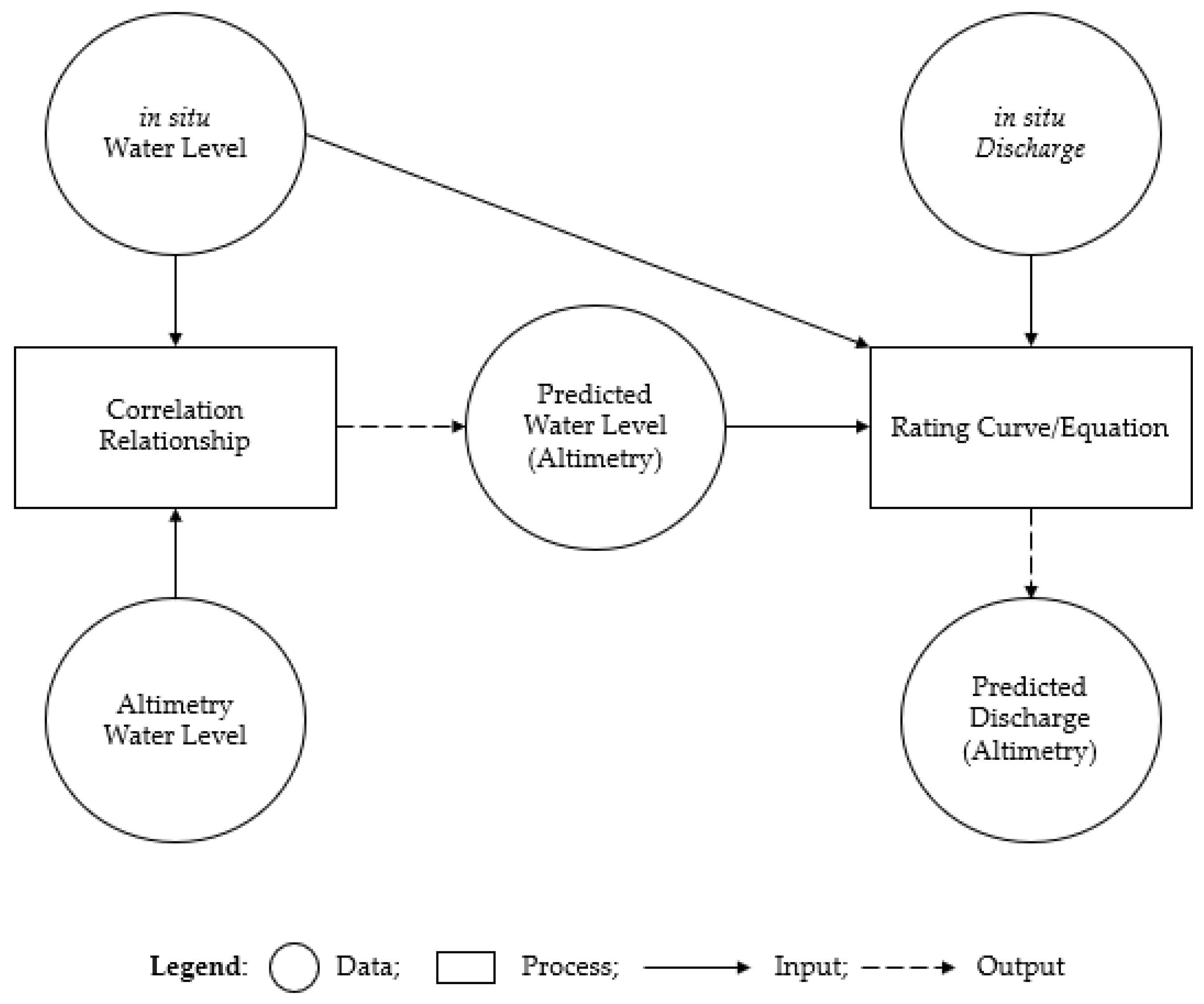
3.3. Missing Data Imputation, Pre-Processing, and Flood Frequency Analysis

3.3.1. Radar Altimetry Data Processing

The approach adopted establishes a relationship between upstream or downstream RA virtual station datasets and a nearby in situ gauging station datasets when water level data exist at both stations on the same date. The established correlation equation was then applied to estimate missing in situ data when only RA data is available, which is then converted to discharge using an up-to-date rating curve. At locations where in situ and/or RA data is not available for the same dates to establish an empirical relationship, a previously established relationship from a nearby RA station was adopted, provided no tributary or distributary exists between both virtual stations, the change in river width is minimal, and no hydraulic structure or tributary exists between both virtual stations [35,57]. This approach is consistent with previous studies [57,58], where the rating curve for a nearby gauging station was adopted for another station where data was unavailable. In this study, this altimetry/in situ relation transfer approach was adapted for Umaisha station and Virtual station Env_158_01 (Table 3), where the relationship established from Jason 2 data was applied to Envisat data. The framework presented in Figure 2 describes the methodology for infilling missing data using RA, while the characteristics of RA virtual stations and the derived regression relationships are presented in Table 3.

3.3.2. Multiple Imputation of Missing Data

MI allows for the infilling of missing data in situations where altimetry virtual stations are unavailable and has been widely applied in hydrological studies [27,59]. MI has also been found to outperform traditional techniques such as mean imputation, missing indicator, and complete case analysis [60,61], hence its selection for this research. MI fills data gaps by simulating the plausible number of values after fitting the existing data to a distribution based on the statistical parameters such as mean and standard deviation of the dataset while accounting for uncertainty about the supposed true value [62,63]. The term “multiple imputation” implies the missing data is simulated multiple times, in this case, five times using XLSTAT software, which is considered sufficient from previous studies [64]. Markov chain Monte Carlo approach is applied to estimate missing values by randomly sampling from a distribution of plausible values derived from multiple simulations undertaken using mean and standard error parameters similar to that of the original dataset under the assumption of normal distribution [65]. This approach quantifies the uncertainty in the simulation process and reduces false precision attainable with single imputation [62]. A major limitation of this approach is that a small sample size may constrain the generalization potential of the imputation method proposed, thus resulting in uncertain missing data estimates [66].
At locations where RA data was not available for certain years to reflect peak floods, MI was applied to infill the remaining gaps. For instance, Baro (11 missing: 1 filled with RA, 10 filled with MI), Lokoja (6 Missing: 6 filled with RA), Umaisha (19 missing: 14 filled with RA, 5 filled with MI), and Onitsha (16 missing: 9 filled with RA, 7 with MI).

3.3.3. Hydrological Data Pre-Processing

Preliminary analysis is a prerequisite for most flood frequency analyses studies, to assess the likely factors that contribute to flood estimate uncertainties [67,68,69]. These analyses generally include tests for outliers, trends, homogeneity, serial correlation, and rating curve extrapolation effects. The five tests undertaken in this study include:
  • Grubbs and Becks [70] and Multiple Grubbs and Becks outlier test [71]: to identify Potentially Influential Low Floods (PILFs);
  • Mann–Kendall test [72,73]: to assess trends in the time-series;
  • Pettitt’s test [74]: to assess historical data homogeneity;
  • One-unit lag correlation coefficient statistics [75]: to test the serial correlation between the independent observations of a time-series,
  • Ratings Ratio [76]: to assesses possible rating curve extrapolation effects by dividing the maximum discharge for each year by the maximum measured discharge applied in the ratings curve development.
All data pre-processing, except the multiple Grubbs and Becks test (mGBt), was undertaken using XLSTAT software, while mGBt was performed in Flike flood frequency analysis software [67,77]. A vast body of literature is available on fundamental theories and methodologies of this preliminary analysis for further perusal; hence is not discussed in detail here.

3.3.4. Flood Frequency Estimation

Flood frequency analysis (FFA) was undertaken in Flike software [77] by fitting a pre-defined probability distribution (generalized extreme value (GEV)) to both gap-filled and unfilled historic annual maximum series (AMS) data derived from the RA and MI approaches, to determine flood return period, i.e., the likelihood of a flood of specific magnitude being met or exceeded at any given point in time [78]. Different probability distributions including generalized extreme value (GEV), generalized logistic (GLO), extreme value (type 1–3), generalized Pareto (GPA), and log Pearson type 3 (LP3) have been widely applied for FFA, and provide varying flood estimates, even for the same dataset [79]. Hence, suitability analysis is typically undertaken to access the best probability distribution [80]. Nonetheless, GEV is adopted for FFA in this study, due to its robustness, flexibility [81,82] and for consistency with previous studies in our area of interest [83,84]. The GEV formula is expressed as
F   ( x | τ , α , k ) = [ 1 α exp { [ 1 k ( x τ ) α ] 1 k }   [ 1 k ( x τ ) α ] 1 k 1 ;   when   k > 0 ,   x < τ + α k ; when   k < 0 ,   x > τ + α k 1 α exp [ 1 ( x τ ) α ] exp { exp [ ( x τ ) α ] } ; if   k = 0
where, τ, α, and k represents location, scale and shape parameters of the distribution function.
GEV like other probability distributions is affected by short hydrological time series, which results in uncertain flood estimates [85], therefore the availability of more historical data enables improved flood estimation. The 5T rule of thumb suggested by Reed [78] for the length of data required for flood frequency estimation is adopted for this study, i.e., the historical data should be at least five times the target return periods (i.e., 20 years of historical data is required for a 1-in-100-year estimation, for reasonable levels of uncertainty).

3.3.5. Assessment of Missing Data Imputation Method Impact on Flood Frequency Estimates

Permutation and Kolmogorov–Simonov tests were undertaken in R software to assess the effect of the various missing data imputation approaches on the flood estimates, as well as the respective quantile distributions. The permutation test is the non-parametric alternative to the parametric t-test, used in evaluating the difference between two treatments [86], in this case, RA and MI, while the Kolmogorov–Simonov test assesses if two distributions are similar or if a distribution differs from a reference distribution [87].

3.5.6. Missing Data Imputation Methodology Outcome Evaluation

To further evaluate the effect of the infilling approaches on flood estimates, complete hydrological time series available at Taoussa gauging station in Mali, West Africa (location map in Supplementary Figure S1) was acquired from the Niger Basin Authority data repository via the web link: http://nigerhycos.abn.ne/user-anon/htm/, due to the absence of gap-free data in Nigeria. Historical water levels were converted to discharge using a ratings curve. Known data points were deliberately removed to reflect missing data patterns evident in existing Nigerian datasets, i.e., consecutive (≤3 years) and inconsecutive (>3 years), then filled with the MI and RA approaches, and applied for flood frequency estimation. The discordancy between flood estimates derived from the filled and original complete datasets was then evaluated using Permutation and Kolmogorov–Simonov tests.

4. Results and Discussion

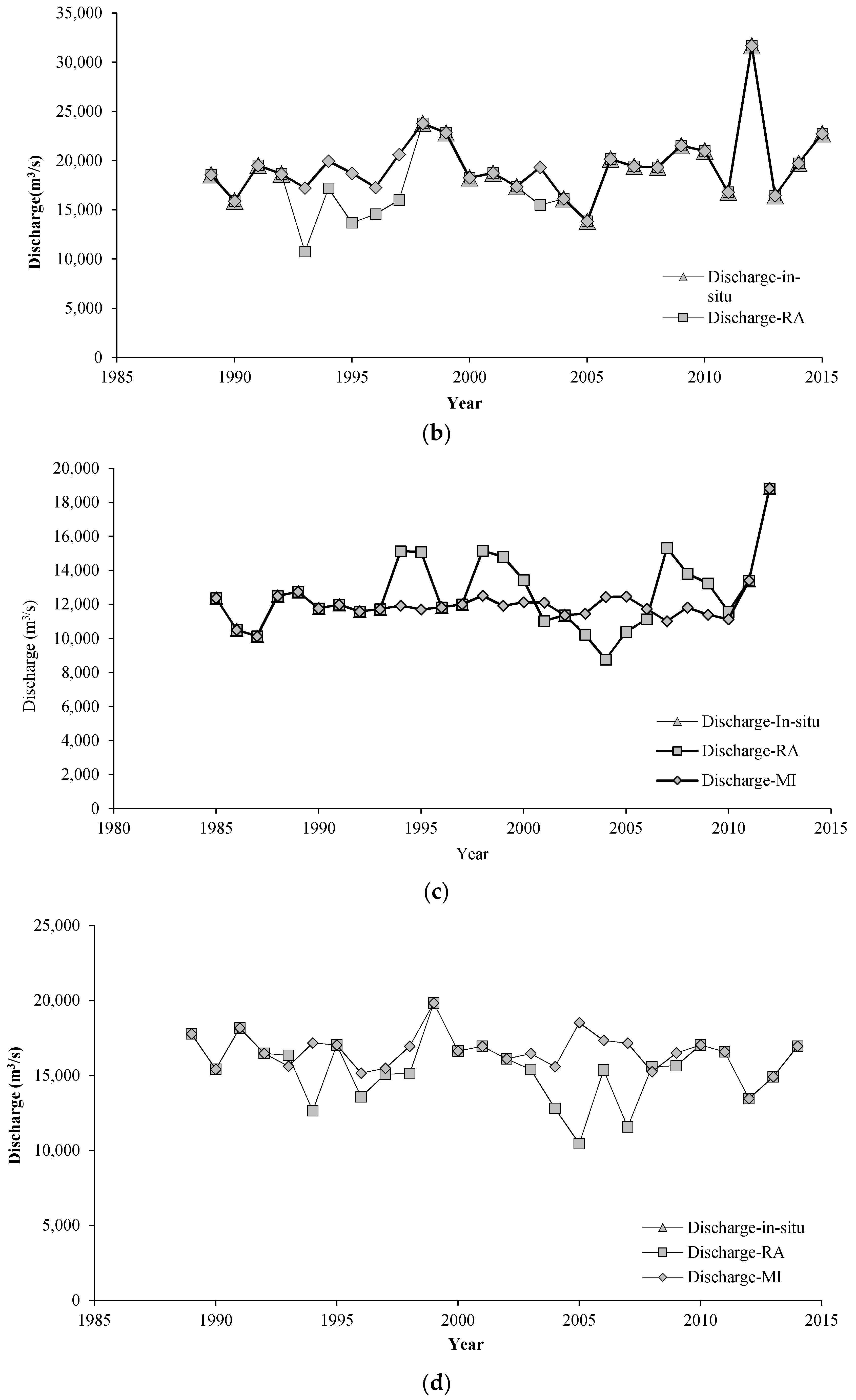
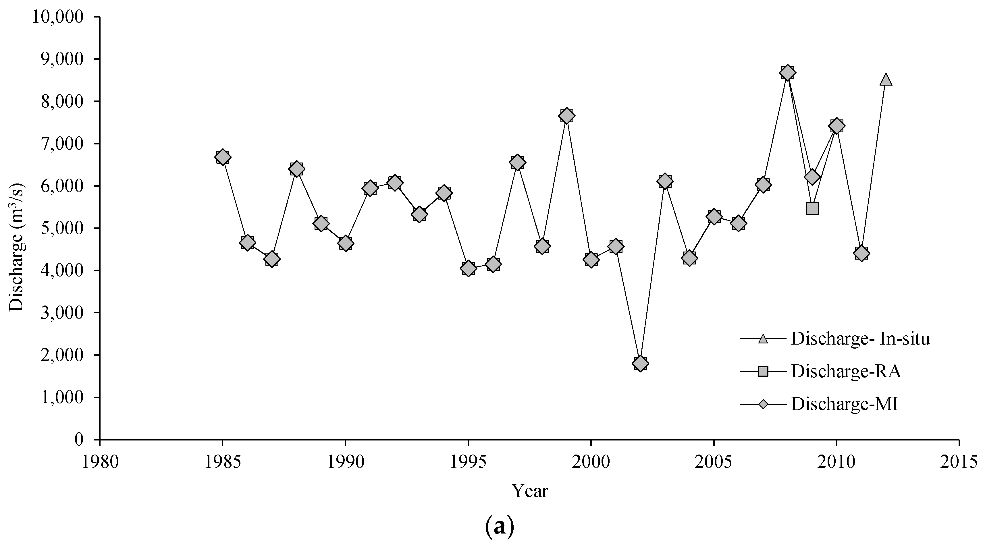
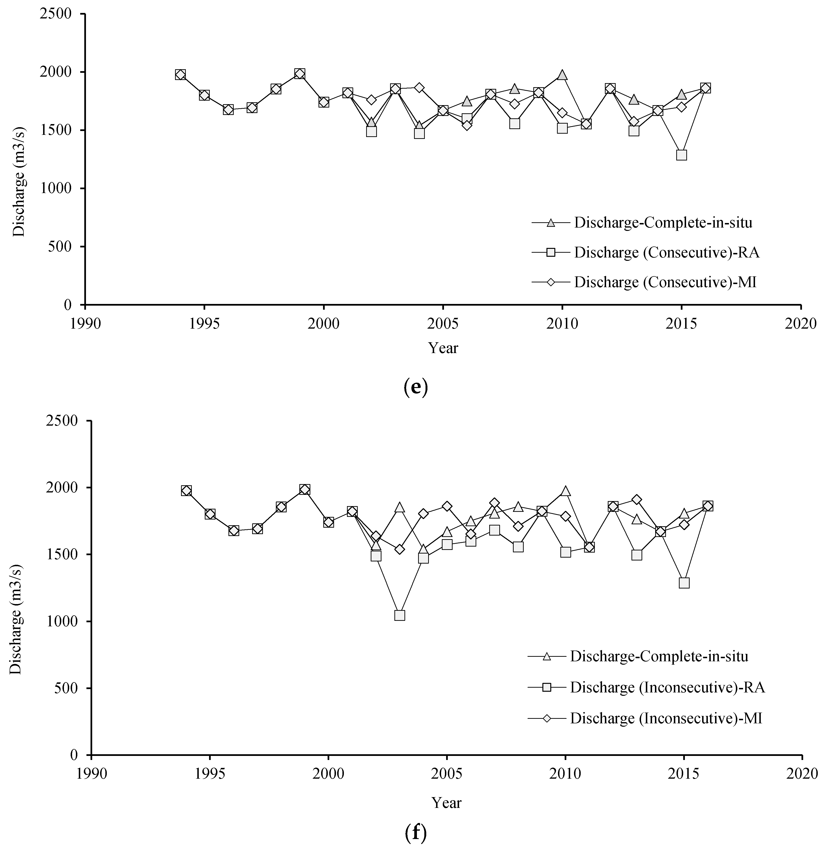
4.1. Missing Data Infilling with Radar Altimetry and Multiple Imputation

The coefficients of determination (R2) for the relationship between RA and in situ water level data points presented in Table 3 were higher at gauging stations where the distances between virtual and in situ gauge stations was minimal, as well as where the influence of tributaries discharging into the main rivers is reduced and river width is considerable. These are evident at j2_020_1 (R2 = 0.947) and tp198_4_moy (R2 = 0.659) virtual stations for Lokoja and Onitsha, respectively. The Jason Virtual station (j2_020_1) is located 115.4 Km upstream from Lokoja along the Niger river stretch, with no tributary influence and at a river cross-sectional width of 2.37 Km, while the Topex/Poseidon Virtual station (tp198_4_moy) is located 234.7 Km downstream of Onitsha, influenced by Nun and Anambra river tributaries, and at a river cross-sectional width of 0.47 Km. These findings are consistent with studies at Brahmaputra River [88], Lake Argyle [34], Lake Victoria [34,38,88], and Benue River [35], where the distance between in situ and RA virtual stations, existence of tributaries between the stations, and river width impacted the correlation between datasets.
Figure 3a–d shows the annual maximum timeseries data for the four gauging stations in Nigeria for gapped and infilled datasets. Triangular markers depict point where historical in situ data exist, while MI and RA derived estimates are depicted as diamond-like and square markers, respectively. The RA derived missing peak discharge values were consistently higher than MI estimates at Umaisha, especially for inconsecutive gaps likely caused by restricted access to gauging stations and equipment damage during peak flood periods. The consistently low peak flood estimates displayed for MI derived estimates at Umaisha reveal the deficiency of MI, especially when estimating missing data for time series with wide gaps greater than three years [29]. At Baro, Lokoja, and Onitsha gauging stations, RA peak flood estimates were generally lower than those estimated by MI, and higher only in 1993 and 2008 at Onitsha. The peak flood values estimated using MI remained relatively steady over time, while RA exhibited high levels of variability expected for natural flood hydrographs, especially for datasets with wide gaps greater than three years as seen at Umaisha. Figure 3e–f shows the timeseries for the Taoussa reference station in Mali, used to validate the methods applied to fill consecutively and inconsecutively gapped historical time-series. Both figures reveal that estimated peak discharge was discordant from the real discharge values, but RA estimates were closer to the actual measurements in comparison to MI estimates for both consecutively and inconsecutively gapped datasets.

4.2. Preliminary Data Analysis

Results of the preliminary analysis are presented in Table 4 and show the statistical parameters that define outliers, trends, homogeneity, and serial correlation of the hydrological datasets for each gauging station. Table 4 reveals (i) the Grubbs and Becks, and Multiple Grubbs and Becks outlier test disclosed the absence of significant potentially influential low flow outliers within the dataset (p > 0.05), inferring that low flows are also drawn from the same sample population. Also, high flows are consistent with years of recorded flood events, hence did not emanate from equipment failure or documentation error; (ii) the Mann–Kendall trend test demonstrated the absence trends for all gauging stations at a significance level (α) greater than 5%; (iii) the homogeneity (Pettitt) test suggests stationarity due to the absence of significant breakpoints within the historical data for each site; and (v) serial (1-unit lag) correlation between peak floods for each site varied from −0.044 to 0.519, suggesting the absence of statistically significant correlation. Positive 1-unit lag correlation infers persistent trends, i.e., high values tend to follow high values and low values tend to follow low values, and negative one-unit lag correlation depicts the reverse [89]. These findings portray the long-term consistency of hydro-physical conditions for the investigated catchment over the period of data collection along Niger and Benue rivers [51,90]. The Ratings Ration (RR) analysis for peak flood data derived from the two infilling approaches (MI and RA) suggests the absence significant rating curve extrapolation uncertainty, as all RR values were not much greater than (>>) 1 as stipulated by Haque et al. [69]. The maximum RR values observed at each gauging station varied from 1.0172 (Baro), 0.8779 (Lokoja), 0.760 (Umaisha), 0.9817 (Onitsha), to 1.045 (Taoussa), which are not much greater than 1.

4.3. Flood Frequency Estimation, Uncertainties, and Application

Flood estimates with upper and lower uncertainty bounds based on a 90% confidence interval (pre-defined in the Flike Software used) for five return periods are presented in Table 5, Table 6, Table 7 and Table 8 and the flood frequency plots are presented as supplementary information. Results from Lokoja and Umaisha present interesting cases for evaluation, given that for Lokoja an equal number of missing data were filled with RA and MI approaches, hence there is an equal base for comparison, while Umaisha has the most missing data (gaps).
The difference between flood estimates derived from in situ datasets with gaps and those filled with MI and RA tend to increase with increasing return periods, and these differences are more pronounced for inconsecutively gapped historic timeseries such as Umaisha (Table 7). At Umaisha, the MI approach resulted in much lower flood estimates than RA, which is consistent with the acknowledged deficiency of MI for estimating missing data for widely gapped datasets [29]. Flood frequency estimated derived from in situ data resulted in higher discharge estimates compared to RA and MI, likely caused by high extrapolation error [91]. At Lokoja where an equal number of data gaps were filled with both MI and RA, the results presented in Table 6 reveal that discharge estimates derived from RA were lower than MI and in situ estimates for the low return periods, and greater than MI for return periods from 1-in-20 to 100-year estimates but remained less than in situ data estimates. Similar trends were observed at Onitsha (Table 8), where out of the 16 missing data points, 9 was available for infilling using RA. At Baro (Table 5), most of the missing datasets were filled with MI due to the absence of continuous RA data, therefore the difference between MI RA, and in situ data flood estimates did not differ significantly. These outcomes infer that both methods can be applied interchangeably for consecutively gapped time-series (≤3 years), and RA and MI can be integrated to improve flood estimates for data-sparse regions.

4.4. Assessment of the Effects of Data Infilling Methods on Flood Quantile Estimates

The results of the Permutation and Kolmogorov–Simonov (K–S) tests presented in Table 9 and Table 10 respectively, assess the statistical significance of the effect of data gaps and the different data infilling approaches on flood frequency estimates. For permutation, the null hypothesis is that there is no difference between the flood frequency estimates derived from data filled using the different approaches, while the alternative hypothesis suggests the contrary. Hence, if the p-value is greater than 0.05, the null hypothesis is confirmed; otherwise, the alternative hypothesis is acceptable [86]. Permutation test results in Table 9 show that p-values for all sites were greater than the significance level of 0.05, confirming the null hypothesis that suggests that the difference between flood estimates derived from data filled using the different approaches, as well the in situ data, did not differ significantly.
Nevertheless, further analysis of the mean difference in water levels (converted from discharge using rating equations) between flood estimates derived from data with gaps filled using RA and MI showed reduce discordancy when compared to RA vs. in situ and MI vs. in situ outcomes, especially for gauging stations with inconsecutively gapped historical data. For instance, at Lokoja where the 6-missing data were equally filled using both RA and MI, the mean difference in discharge resulted in a water level difference of 1.78 m for RA vs. MI, and the deletion of missing data points resulted in increased water level difference of 4.22 m for RA vs. in situ and 3.56 m for MI vs. in situ data sets. At Umaisha, RA derived flood estimates differed from MI and in situ estimates by 4.66 m and 5.21 m respectively. The differences in mean difference in water level for RA vs. MI is seen to be consistent with the gaps in the historical hydrological data used to derive flood frequency estimates, larger with wider inconsecutive gaps >3 years and vice versa. Differences in mean difference in water levels for RI vs. in situ and MI vs. in situ were also large for both consecutively and inconsecutively gapped data, suggesting that use of historical data without gaps being filled will result in discordant flood estimates due to increased extrapolation uncertainty [92].
The K–S test null hypothesis suggests that the two samples were drawn from the same distribution or do not differ from a reference distribution, and the alternative hypothesis dictates otherwise. If the p-value is greater than α = 0.05, the null hypothesis is confirmed; otherwise, the alternative hypothesis is accepted. The D statistic is the absolute maximum distance between the cumulative distribution functions of the two samples. The closer this number is to 0 the more likely it is that the two samples were drawn from the same distribution [87]. Results from Table 10 reveals that probability distribution was not statistically different (p > 0.05), and hence it does not differ from the pre-selected reference GEV distribution.

4.5. Assessment of Radar Altimetry and Multiple Imputation Infilling at Taoussa, Mali

Flood frequency estimates and the upper and lower uncertainty bounds for 1-in-2 to 1-in-100-year flood events are presented in Table 11 to capture varying scenarios of gaps (consecutive and inconsecutive) filled using RA and MI. The results show that flood estimates for both infilling approaches are within the 90% confidence interval bounds of flood estimates derived from the original complete data for all return periods, except for the 1-in-2-year flood estimates derived from consecutively and inconsecutively gapped data filled with RA. Permutation and Kolmogorov–Simonov test results (Table 12) further revealed that although discharge estimates did not significantly differ (Pperm > 0.05), the difference between water levels derived from RA and MI infilled datasets was up to 2 m for both consecutively and inconsecutively gapped datasets. Also, the Dks and Pks-Values for the RA-infilled estimates for both consecutive and inconsecutively gapped time series showed significant differences in distribution when compared to the original complete data. The observed difference in distribution suggests that the complete and RA-infilled flood estimates are not drawn from the same distribution despite not being significantly different [93]. Therefore, an assessment of the optimal probability distribution for fitting the data from the varying infilling approaches is recommended, rather than using a predefined distribution such as GEV as was the case in this study, given that different probability distributions can result in very different flood estimates, even for the same dataset [79].

4.6. The 2012 Flood Event Return Period Estimations

A retrospective approach was undertaken in this study to characterize the magnitude of the 2012 flood event that resulted in devastating impacts, having filled the data gaps using RA which was identified as the most appropriate of the techniques compared herein. The results presented Table 13 reveal that the peak values for the gauging stations measuring discharge into the Niger-South river basin were within the 90% confidence level of the lower uncertainty bounds of a 1-in-50-year flood for Baro (8533 m3/s) and Lokoja (31,692 m3/s), and a 1-in-100-year flood for Umaisha (18,816 m3/s). This suggests that higher flood magnitudes emanated from the Benue river, likely from excess water releases from the Lagdo and Kiri dams in Cameroon and Nigeria, respectively, as previously suspected to be the cause of the 2012 flood event [47,49]. Nigeria is currently experiencing flooding in 2018, and the non-release of water from upstream Lagdo dam has proven significant in ensuring current flood levels along river Benue are less than those experienced in 2012. In a statement released by the Nigerian Hydrological Service Agency, “The Lagdo Dam in Cameroon is still impounding water and has not started spilling water into River Benue” [50]. This goes further to show the value of transboundary flood monitoring and early warning, and its applicability across various transboundary river basins [6].

5. Conclusions

Missing data is a recurring challenge for flood management in many developing regions, where hydrological data is often manually collected and where peak flood events result in restricted access for data collection and damage to measuring equipment. In other cases, gauging stations are newly established and have short datasets that cannot be applied for flood frequency estimation. The results of this study suggest that RA and MI can be used to fill such missing data gaps, depending on the size of the missing data and the availability of additional information for satellite altimetry. RA-infilled discharge datasets have higher variability than MI-infilled data and is consistent with natural flood hydrographs. RA infilling also outperformed MI infilling for consecutively gapped datasets with missing data for ≥3 years, and the use of in situ datasets with missing data can result in higher flood estimates with widened uncertainty margins for high return periods. For MI, a small sample size may constrain the generalization potential of the imputation method, thus resulting in uncertain missing data estimates [66]. For consecutively gapped hydrological time series with missing data for ≤3 years, RA and MI infilling approaches performed similarly and can be applied interchangeably. The infilled data facilitated the quantification of the magnitude of the 2012 flood event for the three gauging stations along the Niger and Benue rivers. This revealed that higher flood magnitudes emanated from the Benue river, likely from excess water release from dams in Cameroon and Nigeria, suggesting the need for improved upstream dam management, early warning, and communication systems.
RA showed considerable potential for improving hydrological data collection and modelling in this study and would also be useful for the reconstruction of historical hydrological data for newly established gauging stations if virtual station locations are considered during hydrological gauging station network planning. However, with RA, if a flood event occurs between two satellite passes the uncertainty of RA data will be high, consequently impacting flood estimates [12]. Nevertheless, improved RA temporal resolution from missions such as Jason-3, Sentinel-3, and the proposed SWOT is expected to help curb such deficiencies and increased data availability through enhanced in situ monitoring networks and historical data reconstruction using RA can help increase the sample size available to implement MI with reduced uncertainty. Hence, the synergistic use of RA and MI holds considerable promise for alleviating the problems of hydrological data sparsity in developing regions.

Supplementary Materials

The following are available online at https://www.mdpi.com/2073-4441/10/10/1483/s1, Figure S1: Location of in situ Taoussa in relation to Altimetry virtual station.

Author Contributions

I.T.E.-w. and G.A.B. conceived and designed the study; I.T.E.-w. performed the altimetry and statistical and flood frequency analysis, with guidance from G.A.B. and P.P.; I.T.E.-w. drafted this manuscript, and G.A.B. and P.P. reviewed and provided constructive feedback and input for improvement.

Funding

The authors acknowledge the Niger Delta Development Commission (NDDC), Nigeria for funding I.T.E.-w.’s PhD at Lancaster University, UK (NDDC/DEHSS/2013PGFS/BY/5), from which this paper is a product.

Acknowledgments

The authors acknowledge the Niger Delta Development Commission (NDDC), Nigeria for funding I.T.E.-w.’s PhD at Lancaster University, UK (NDDC/DEHSS/2013PGFS/BY/5), from which this paper is a product; We also acknowledge The Nigerian Hydrological Service Agency (NIHSA), National Inland Waterways Authority (NIWA) and the Niger Basin Authority (NBA) for providing the in situ river hydrological data and the Centre for Topological studies of the Ocean and Hydrosphere (CTOH) for availing off-the-shelf RA data. BMT WBM, Australia for provided free Flike software license used for flood frequency analysis and provided other technical support and guidance. The authors also appreciate the two anonymous reviewers for providing valuable feedback that resulted in the improvement of this article.

Conflicts of Interest

The authors declare no conflict of interest.

References

  1. Lavender, S.L.; Matthews, A.J. Response of the West African Monsoon to the Madden-Julian Oscillation. J. Clim. 2009, 22, 4097–4116. [Google Scholar] [CrossRef]
  2. Bshir, D.; Garba, M. Hydrological Monitoring and Information System for Sustainable Basin Management. In Proceedings of the First Annual Conference of the Nigerian Association of Hydrological Sciences, Yola, Nigeria, 2–4 December 2003. [Google Scholar]
  3. Herschy, R.W. Streamflow Measurement, 3rd ed.; Taylor & Francis: New York, NY, USA, 2008. [Google Scholar]
  4. Olayinka, D.N.; Nwilo, P.C.; Emmanuel, A. From Catchment to Reach: Predictive Modelling of Floods in Nigeria. In Proceedings of the FIG Working Week 2013, Environment for Sustainability, Abuja, Nigeria, 6–10 May 2013. [Google Scholar]
  5. Giustarini, L.; Parisot, O.; Ghoniem, M.; Hostache, R.; Trebs, I.; Otjacques, B. A User-Driven Case-Based Reasoning Tool for Infilling Missing Values in Daily Mean River Flow Records. Environ. Model. Softw. 2016, 82, 308–320. [Google Scholar] [CrossRef]
  6. Ekeu-Wei, I.T.; Blackburn, G.A. Applications of Open-Access Remotely Sensed Data for Flood Modelling and Mapping in Developing Regions. Hydrology 2018, 5, 39. [Google Scholar] [CrossRef]
  7. Merz, B.; Thieken, A.H. Separating Natural and Epistemic Uncertainty in Flood Frequency Analysis. J. Hydrol. 2005, 309, 114–132. [Google Scholar] [CrossRef]
  8. Tarpanelli, A.; Brocca, L.; Lacava, T.; Melone, F.; Moramarco, T.; Faruolo, M.; Pergola, N.; Tramutoli, V. Toward the Estimation of River Discharge Variations Using Modis Data in Ungauged Basins. Remote Sens. Environ. 2013, 136, 47–55. [Google Scholar] [CrossRef]
  9. Birkinshaw, S.J.; Moore, P.; Kilsby, C.G.; Donnell, G.M.; Hardy, A.J.; Berry, P.A.M. Daily Discharge Estimation at Ungauged River Sites Using Remote Sensing. Hydrol. Process. 2014, 28, 1043–1054. [Google Scholar] [CrossRef]
  10. Neal, J.; Schumann, G.; Bates, P. A Subgrid Channel Model for Simulating River Hydraulics and Floodplain Inundation over Large and Data Sparse Areas. Water Resour. Res. 2012, 48. [Google Scholar] [CrossRef]
  11. Pereira Cardenal, S.J.; Riegels, N.; Berry, P.; Smith, R.; Yakovlev, A.; Siegfried, T.; Bauer-Gottwein, P. Real-Time Remote Sensing Driven River Basin Modelling Using Radar Altimetry. Hydrol. Earth Syst. Sci. 2010, 7, 8347–8385. [Google Scholar] [CrossRef] [Green Version]
  12. Jarihani, A.A.; Larsen, J.R.; Callow, J.N.; Mcvicar, T.R.; Johansen, K. Where Does All the Water Go? Partitioning Water Transmission Losses in a Data-Sparse, Multi-Channel and Low-Gradient Dryland River System Using Modelling and Remote Sensing. J. Hydrol. 2015, 529, 1511–1529. [Google Scholar] [CrossRef]
  13. Jotish, N.; Parthasarathi, C.; Nazrin, U.; Victor, S.K.; Silchar, A. A Geomorphological Based Rainfall-Runoff Model for Ungauged Watersheds. Int. J. Geomat. Geosci. 2011, 2, 676–687. [Google Scholar]
  14. Smith, A.; Sampson, C.; Bates, P. Regional Flood Frequency Analysis at the Global Scale. Water Resour. Res. 2015, 51, 539–553. [Google Scholar] [CrossRef]
  15. Hrachowitz, M.; Savenije, H.; Blöschl, G.; Mcdonnell, J.; Sivapalan, M.; Pomeroy, J.; Arheimer, B.; Blume, T.; Clark, M.; Ehret, U. A Decade of Predictions in Ungauged Basins (Pub)—A Review. Hydrol. Sci. J. 2013, 58, 1198–1255. [Google Scholar] [CrossRef]
  16. Jung, Y.; Merwade, V. Estimation of Uncertainty Propagation in Flood Inundation Mapping Using a 1-D Hydraulic Model. Hydrol. Process. 2015, 29, 624–640. [Google Scholar] [CrossRef]
  17. Campozano, L.; Sánchez, E.; Aviles, A.; Samaniego, E. Evaluation of Infilling Methods for Time Series of Daily Precipitation and Temperature: The Case of the Ecuadorian Andes. Maskana 2014, 5, 99–115. [Google Scholar]
  18. Westerberg, I.; Mcmillan, H. Uncertainty in Hydrological Signatures. Hydrol. Earth Syst. Sci. 2015, 12, 4233–4270. [Google Scholar] [CrossRef]
  19. Lee, H.; Kang, K. Interpolation of Missing Precipitation Data Using Kernel Estimations for Hydrologic Modeling. Adv. Meteorol. 2015, 2015, 935868. [Google Scholar] [CrossRef]
  20. Hasan, M.M.; Croke, B. Filling Gaps in Daily Rainfall Data: A Statistical Approach. In Proceedings of the 20th International Congress on Modelling and Simulation (MODSIM2013), Adelaide, Australia, 1–6 December 2013; pp. 380–386. [Google Scholar]
  21. Steven, K.S.; Shelli, K.S.T.H.; Travis, H.; Yunsheng, S.; Denny, T.; Mark, B. Filling in Missing Peakflow Data Using Artificial Neural Networks. J. Eng. Appl. Sci. 2010, 5, 49–55. [Google Scholar]
  22. Peugh, J.L.; Enders, C.K. Missing Data in Educational Research: A Review of Reporting Practices and Suggestions for Improvement. Rev. Educ. Res. 2004, 74, 525–556. [Google Scholar] [CrossRef]
  23. King, G.; Honaker, J.; Joseph, A.; Scheve, K. List-Wise Deletion is Evil: What to Do about Missing Data in Political Science. In Proceedings of the Annual Meeting of the American Political Science Association, Boston, MA, USA, 19 August 1988. [Google Scholar]
  24. Little, R.J.A. Statistical Analysis with Missing Data, 2nd ed.; Wiley: Hoboken, NJ, USA, 2002. [Google Scholar]
  25. Donders, A.R.T.; Van Der Heijden, G.J.M.G.; Stijnen, T.; Moons, K.G.M. Review: A Gentle Introduction to Imputation of Missing Values. J. Clin. Epidemiol. 2006, 59, 1087–1091. [Google Scholar] [CrossRef] [PubMed]
  26. Jolliffe, I.T. Principal Component Analysis [Electronic Resource], 2nd ed.; Springer: New York, NY, USA, 2002. [Google Scholar]
  27. Graham, J.; Olchowski, A.; Gilreath, T. How Many Imputations Are Really Needed? Some Practical Clarifications of Multiple Imputation Theory. Prev. Sci. 2007, 8, 206–213. [Google Scholar] [CrossRef] [PubMed]
  28. Khalifeloo, M.H.; Mohammad, M.; Heydari, M. Multiple Imputation for Hydrological Missing Data by Using a Regression Method (Klang River Basin). Int. J. Res. Eng. Technol. 2015, 4, 519–524. [Google Scholar]
  29. Tyler, C.M.; Sue Ellen, H.; George, S.Y. The Effects of Imputing Missing Data on Ensemble Temperature Forecasts. J. Comput. 2011, 6, 162–171. [Google Scholar]
  30. Lee, K.J.; Carlin, J.B. Multiple Imputation for Missing Data: Fully Conditional Specification Versus Multivariate Normal Imputation. Am. J. Epidemiol. 2010, 171, 624–632. [Google Scholar] [CrossRef] [PubMed] [Green Version]
  31. Pan, F.; Nichols, J. Remote Sensing of River Stage Using the Cross-Sectional Inundation Area-River Stage Relationship (Iarsr) Constructed from Digital Elevation Model Data. Hydrol. Process. 2013, 27, 3596–3606. [Google Scholar] [CrossRef]
  32. Tommaso, M.; Angelica, T.; Luca, B.; Silvia, B. River Discharge Estimation by Using Altimetry Data and Simplified Flood Routing Modeling. Remote Sens. 2013, 5, 4145–4162. [Google Scholar] [Green Version]
  33. Gleason, C.J.; Smith, L.C. Toward Global Mapping of River Discharge Using Satellite Images and at-Many-Stations Hydraulic Geometry. Proc. Natl. Acad. Sci. USA 2014, 111, 4788–4791. [Google Scholar] [CrossRef] [PubMed]
  34. Asadzadeh Jarihani, A.; Callow, J.N.; Johansen, K.; Gouweleeuw, B. Evaluation of Multiple Satellite Altimetry Data for Studying Inland Water Bodies and River Floods. J. Hydrol. 2013, 505, 78–90. [Google Scholar] [CrossRef]
  35. Pandey, R.; Amarnath, G. The Potential of Satellite Radar Altimetry in Flood Forecasting: Concept and Implementation for the Niger-Benue River Basin. Proc. IAHS 2015, 370, 223–227. [Google Scholar] [CrossRef]
  36. Silva, J.; Calmant, S.; Seyler, F.; Moreira, D.; Oliveira, D.; Monteiro, A. Radar Altimetry Aids Managing Gauge Networks. Water Resour. Manag. 2014, 28, 587–603. [Google Scholar] [CrossRef]
  37. Osti, R.; Tanaka, S.; Tokioka, T. Flood Hazard Mapping in Developing Countries: Problems and Prospects. Disaster Prev. Manag. Int. J. 2008, 17, 104–113. [Google Scholar] [CrossRef]
  38. Crétaux, J.-F.; Jelinski, W.; Calmant, S.; Kouraev, A.; Vuglinski, V.; Bergé-Nguyen, M.; Gennero, M.-C.; Nino, F.; Del Rio, R.A.; Cazenave, A. Sols: A Lake Database to Monitor in the near Real Time Water Level and Storage Variations from Remote Sensing Data. Adv. Space Res. 2011, 47, 1497–1507. [Google Scholar] [CrossRef]
  39. NESDIS. Jason 3 Has Reached Its Operational Orbit. 2016. Available online: http://www.nesdis.noaa.gov/news_archives/jason3_lift_off_is_just_the_beginning.html (accessed on 20 February 2016).
  40. European Space Agency (ESA). Third Sentinel Launch for Copernicus. 2016. Available online: http://www.esa.int/Our_Activities/Observing_the_Earth/Copernicus/Sentinel-3/Third_Sentinel_satellite_launched_for_Copernicus (accessed on 20 February 2016).
  41. Avisio. Avisio Satellite Altimetry Data. 2016. Available online: http://www.aviso.altimetry.fr/en/home.html (accessed on 1 January 2016).
  42. Clark, E.A.; Sylvainhossain, F.; Jean-Françoislettenmaier, D.P. Altimetry Applications to Transboundary River Basin Management. In Inland Water Altimetry; Benveniste, J., Vignudelli, S., Kostianoy, A., Eds.; Springer: Washington, DC, USA, 2014. [Google Scholar]
  43. Odunuga, S.; Adegun, O.; Raji, S.; Udofia, S. Changes in Flood Risk in Lower Niger-Benue Catchments. Proc. Int. Assoc. Hydrol. Sci. 2015, 370, 97–102. [Google Scholar] [CrossRef]
  44. The Project for Review and Update of Nigeria National Water Resources Master Plan; Federal Ministry of Water Resources: Abuja, Nigeria, 2013.
  45. Post-Disaster Needs Assessment 2012 Floods; The Federal Government of Nigeria: Abuja, Nigeria, 2013.
  46. Erekpokeme, L.N. Flood Disasters in Nigeria: Farmers and Governments’ Mitigation efforts. J. Biol. Agric. Healthc. 2015, 5, 150–154. [Google Scholar]
  47. Ojigi, M.; Abdulkadir, F.; Aderoju, M. Geospatial Mapping and Analysis of the 2012 Flood Disaster in Central Parts of Nigeria. In Proceedings of the 8th National GIS Symposium, Dammam, Saudi Arabia, 15–17 April 2013; pp. 1–14. [Google Scholar]
  48. Tami, A.G.; Moses, O. Flood Vulnerability Assessment of Niger Delta States Relative to 2012 Flood Disaster in Nigeria. Am. J. Environ. Prot. 2015, 3, 76–83. [Google Scholar]
  49. Olojo, O.O.; Asma, T.I.; Isah, A.A.; Oyewumi, A.S.; Adepero, O. The Role of Earth Observation Satellite During the International collaboration on the 2012 Nigeria Flood Disaster. In Proceedings of the 64th International Astronautical Congress, Beijing, China, 23–27 September 2013. [Google Scholar]
  50. Nigerian Hydrological Service Agency. Update on Nihsa Early Flood Warning in Nigeria as at 30th August 2018. 2018. Available online: http://nihsa.gov.ng/2018/08/30/update-on-nihsa-early-flood-warning-in-nigeria-as-at-30th-august-2018/ (accessed on 2 October 2018).
  51. Abam, T.K.S. Modification of Niger Delta Physical Ecology: The Role of Dams and Reservoirs. Hydro-Ecol. Link. Hydrol. Aquat. Ecol. 2001, 266, 19–29. [Google Scholar]
  52. Da Silva, J.S.; Calmant, S.; Seyler, F.; Rotunno Filho, O.C.; Cochonneau, G.; Mansur, W.J. Water Levels in the Amazon Basin Derived from the Ers 2 and Envisat Radar Altimetry Missions. Remote Sens. Environ. 2010, 114, 2160–2181. [Google Scholar] [CrossRef]
  53. Belaud, G.; Cassan, L.; Bader, J.; Bercher, N.; Feret, T. Calibration of a Propagation Model in Large River Using Satellite Altimetry. In Proceedings of the 6th International Symposium on Environmental Hydraulics, Athens, Greece, 23–25 June 2010; pp. 23–25. [Google Scholar]
  54. Musa, Z.; Popescu, I.; Mynett, A. A Review of Applications of Satellite Sar, Optical, Altimetry and Dem Data for Surface Water Modelling, Mapping and Parameter Estimation. Hydrol. Earth Syst. Sci. 2015, 12, 4857–4878. [Google Scholar] [CrossRef]
  55. Frappart, F.; Calmant, S.; Cauhopé, M.; Seyler, F.; Cazenave, A. Preliminary Results of Envisat Ra-2-Derived Water Levels Validation over the Amazon Basin. Remote Sens. Environ. 2006, 100, 252–264. [Google Scholar] [CrossRef] [Green Version]
  56. Jarihani, A.A.; Callow, J.N.; Mcvicar, T.R.; Van Niel, T.G.; Larsen, J.R. Satellite-Derived Digital Elevation Model (Dem) Selection, Preparation and Correction for Hydrodynamic Modelling in Large, Low-Gradient and Data-Sparse Catchments. J. Hydrol. 2015, 524, 489–506. [Google Scholar] [CrossRef]
  57. Papa, F.; Durand, F.; Rossow, W.B.; Rahman, A.; Bala, S.K. Satellite Altimeter-Derived Monthly Discharge of the Ganga-Brahmaputra River and Its Seasonal to Interannual Variations from 1993 to 2008. J. Geophys. Res. Oceans 2010, 115. [Google Scholar] [CrossRef]
  58. Michailovsky, C.I.; Mcennis, S.; Bauer-Gottwein, P.A.M.; Berry, R.; Smith, P. River Monitoring from Satellite Radar Altimetry in the Zambezi River Basin. Hydrol. Earth Syst. Sci. 2012, 16, 2181–2192. [Google Scholar] [CrossRef] [Green Version]
  59. Gill, M.K.; Asefa, T.; Kaheil, Y.; Mckee, M. Effect of Missing Data on Performance of Learning Algorithms for Hydrologic Predictions: Implications to an Imputation Technique. Water Resour. Res. 2007, 43. [Google Scholar] [CrossRef]
  60. Roderick, J.A.L. Regression with Missing X’s: A Review. J. Am. Stat. Assoc. 2011, 87, 1227–1237. [Google Scholar]
  61. Van Der Heijden, G.J.M.G.; Donders, A.R.T.; Stijnen, T.; Moons, K.G.M. Imputation of Missing Values Is Superior to Complete Case Analysis and the Missing-Indicator Method in Multivariable Diagnostic Research: A Clinical Example. J. Clin. Epidemiol. 2006, 59, 1102–1109. [Google Scholar] [CrossRef] [PubMed]
  62. Li, P.; Stuart, E.; Allison, D. Multiple Imputation a Flexible Tool for Handling Missing Data. JAMA 2015, 314, 1966–1967. [Google Scholar] [CrossRef] [PubMed]
  63. Yozgatligil, C.; Aslan, S.; Iyigun, C.; Batmaz, I. Comparison of Missing Value Imputation Methods in Time Series: The Case of Turkish Meteorological Data. Theor. Appl. Climatol. 2013, 112, 143–167. [Google Scholar] [CrossRef]
  64. Sattari, M.-T.; Rezazadeh-Joudi, A.; Kusiak, A. Assessment of Different Methods for Estimation of Missing Data in Precipitation Studies. Hydrol. Res. 2017, 48, 1032–1044. [Google Scholar] [CrossRef]
  65. Van Buuren, S. Multiple Imputation of Discrete and Continuous Data by Fully Conditional Specification. Stat. Methods Med. Res. 2007, 16, 219–242. [Google Scholar] [CrossRef] [PubMed]
  66. Barnes, S.A.; Lindborg, S.R.; Seaman, J.W. Multiple Imputation Techniques in Small Sample Clinical Trials. Stat. Med. 2006, 25, 233–245. [Google Scholar] [CrossRef] [PubMed]
  67. Lamontagne, J.R.; Stedinger, J.R.; Cohn, T.A.; Barth, N.A. Robust National Flood Frequency Guidelines: What Is an Outlier? In Proceedings of the World Environmental and Water Resources Congress, Cincinnati, OH, USA, 19–23 May 2013.
  68. Di Baldassarre, G.; Laio, F.; Montanari, A. Effect of Observation Errors on the Uncertainty of Design Floods. Phys. Chem. Earth 2012, 42–44, 85–90. [Google Scholar] [CrossRef]
  69. Haque, M.M.; Rahman, A.; Haddad, K. Rating Curve Uncertainty in Flood Frequency Analysis: A Quantitative Assessment. J. Hydrol. Environ. Res. 2014, 2, 50–58. [Google Scholar]
  70. Grubbs, F.E.; Beck, G. Extension of Sample Sizes and Percentage Points for Significance Tests of Outlying Observations. Technometrics 1972, 14, 847–854. [Google Scholar] [CrossRef]
  71. Rahman, A.S.; Haddad, K.; Rahman, A. Identification of Outliers in Flood Frequency Analysis: Comparison of Original and Multiple Grubbs-Beck Test. World Acad. Sci. Eng. Technol. 2014, 8, 732–740. [Google Scholar]
  72. Mann, H.B. Nonparametric Tests against Trend. Econom. J. Econom. Soc. 1945, 13, 245–259. [Google Scholar] [CrossRef]
  73. Kendall, M. Rank Correlation Methods, 4th ed.; Charles Griffin: London, UK, 1975. [Google Scholar]
  74. Pettitt, A. A Non-Parametric Approach to the Change-Point Problem. Appl. Stat. 1979, 28, 126–135. [Google Scholar] [CrossRef]
  75. Kendall, M.; Stuart, A. The Advanced Theory of Statistics (Volume 1); Griffin: London, UK, 1969. [Google Scholar]
  76. Haddad, K.; Rahman, A.; Weinmann, P.; Kuczera, G.; Ball, J. Streamflow Data Preparation for Regional Flood Frequency Analysis: Lessons from Southeast Australia. Aust. J. Water Resour. 2010, 14, 17–32. [Google Scholar] [CrossRef]
  77. Kuczera, G. Comprehensive at-Site Flood Frequency Analysis Using Monte Carlo Bayesian Inference. Water Resour. Res. 1999, 35, 1551–1557. [Google Scholar] [CrossRef]
  78. Reed, D. Procedures for Flood Freequency Estimation, Volume 3: Statistical Procedures for Flood Freequency Estimation; Institute of Hydrology: Parker, CO, USA, 1999. [Google Scholar]
  79. Laio, F.; Di Baldassarre, G.; Montanari, A. Model Selection Techniques for the Frequency Analysis of Hydrological Extremes. Water Resour. Res. 2009, 45. [Google Scholar] [CrossRef]
  80. Peel, M.; Wang, Q.J.; Vogel, R.; Mcmahon, T. The Utility of L-Moment Ratio Diagrams for Selecting a Regional Probability Distribution. Hydrol. Sci. J. 2001, 46, 147–155. [Google Scholar] [CrossRef]
  81. Komi, K.; Amisigo, B.A.; Diekkrüger, B.; Hountondji, F.C. Regional Flood Frequency Analysis in the Volta River Basin, West Africa. Hydrology 2016, 3, 5. [Google Scholar] [CrossRef]
  82. Hailegeorgis, T.T.; Alfredsen, K. Regional Flood Frequency Analysis and Prediction in Ungauged Basins Including Estimation of Major Uncertainties for Mid-Norway. J. Hydrol. Reg. Stud. 2017, 9, 104–126. [Google Scholar] [CrossRef]
  83. Izinyon, O.; Ehiorobo, J. L-Moments Approach for Flood Frequency Analysis of River Okhuwan in Benin-Owena River Basin in Nigeria. Niger. J. Technol. 2014, 33, 10–18. [Google Scholar] [CrossRef]
  84. Fasinmirin, J.T.; Olufayo, A.A. Comparison of Flood Prediction Models for River Lokoja, Nigeria. Geophys. Res. Abstr. 2006, 8, 02782. [Google Scholar]
  85. Ragulina, G.; Reitan, T. Generalized Extreme Value Shape Parameter and Its Nature for Extreme Precipitation Using Long Time Series and the Bayesian Approach. Hydrol. Sci. J. 2017, 62, 863–879. [Google Scholar] [CrossRef]
  86. Good, P.I. Permutation Tests: A Practical Guide to Resampling Methods for Testing Hypotheses, 2nd ed.; Springer: New York, NY, USA, 2000. [Google Scholar]
  87. Kolmogorov, A.N. Selected Works of A.N. Kolmogorov; Kluwer Academic Publishers: Dordrecht, The Netherland; Boston, MA, USA, 1991. [Google Scholar]
  88. Dubey, A.K.; Gupta, P.; Dutta, S.; Singh, R.P. Water Level Retrieval Using Saral/Altika Observations in the Braided Brahmaputra River, Eastern India. Mar. Geod. 2015, 38, 549–567. [Google Scholar] [CrossRef]
  89. Andrew, T.J.; Louis, E.; Wei, E.; Qiming, E. Time Series Analysis for Psychological Research: Examining and Forecasting Change. Front. Psychol. 2015, 6, 727. [Google Scholar]
  90. Kang, H.M.; Yusof, F. Homogeneity Tests on Daily Rainfall Series in Peninsular Malaysia. Int. J. Contemp. Math. Sci. 2012, 7, 9–22. [Google Scholar]
  91. Feaster, T.D. Importance of Record Length with Respect to Estimating the 1-Percent Chance Flood. In Proceedings of the 2010 South Carolina Water Resources Conference, Columbia, SC, USA, 13–14 October 2010. [Google Scholar]
  92. Baldassarre, G.D.; Montanari, A. Uncertainty in River Discharge Observations: A Quantitative Analysis. Hydrol. Earth Syst. Sci. 2009, 13, 913–921. [Google Scholar] [CrossRef]
  93. Ewemoje, T.A.; Ewemooje, O. Best Distribution and Plotting Positions of Daily Maximum Flood Estimation at Ona River in Ogun-Oshun River Basin, Nigeria. Agric. Eng. Int. CIGR J. 2011, 13, 1–11. [Google Scholar]
Figure 1. (A) Map of Nigeria showing in situ gauging stations, altimetry virtual stations and tracks along Niger and Benue Rivers. (B) Map of Africa showing Niger Basin imprint on Nigeria. (C) Niger South hydrological area showing tributaries (Niger and Anambra) and distributaries (Nun and Forcados).
Water 10 01483 g001
Figure 2. Methodology for estimating missing discharge data using radar altimetry, in situ water level, and rating curve/equation.
Water 10 01483 g002
Figure 3. (a) Baro station in situ and MI and RA infilled time series. (b) Lokoja station in situ and MI and RA infilled time series. (c) Umaisha station in situ and MI and RA Infilled time series. (d) Onitsha station in situ and MI and RA infilled time series. (e) Taoussa original complete time series and time series with consecutive missing data filled using MI and RA. (f) Taoussa original complete time series and time series with inconsecutive missing data filled using MI and RA.
Water 10 01483 g003aWater 10 01483 g003bWater 10 01483 g003c
Table 1. In situ gauge station characteristics.
Station NameDate EstablishedRiverLat. (°)Long. (°)Area (km2)Period of Record Used (years)GBM (m)River Width
(km)
Missing Annual
Peak Discharge Data
Data Source
Baro1915Niger8.60666.4170730,0001985–201257.220.6412NIHSA
Lokoja1915Niger7.81676.7333752,0001989–201545.771.656NIHSA
Umaisha1980Benue8.00007.2333335,0001985–201218.870.6119NIHSA
Onitsha1955Niger6.16676.75001,100,0001989–201424.141.0316NIWA
Taoussa1954Niger16.9500−0.5800340,0001985–2015N/A0.470NBA
GBM: gauge benchmark above mean sea level, N/A: not applicable (Source: NISHA, NIWA, and NBA).
Table 2. Radar altimetry mission and characteristics.
S/NMissionGround Footprint (m)Return Period (Days)Operation TimelineVertical Accuracy (m)References
1T/P~6009.91993–20030.35[55]
2Envisat~400352002–20120.28[55]
3Jason-1~300102002–20091.07[56]
4Jason-2~300102008–Till date0.28[56]
T/P = Topex/Poseidon.
Table 3. Characteristics of the altimetry virtual stations within the study area.
Virtual Station NameMissionRiverTemporal CoverageLat.Long.Distance from in situ Gauge (km)River Width (km)Available Data Points (Alt vs. in situ)Regression EquationR2
Env_702_01EnvisatNiger2002–20106.65006.6500115.4 (Lokoja)-DS0.4910in situ = 0.8807(RA) + 29.8210.876
Env_029_01EnvisatNiger2002–20105.99006.720023.7 (Onitsha)-DS0.899in situ = 1.1004(RA) + 33.8290.95
Env_158_01EnvisatBenue2002–20108.02007.670054.3 (Umaisha)-US1.7115!in situ = 0.9409 (RA) − 19.6210.947!
tp198_4_moyT/PNun1993–20026.09814.7563234.7 (Onitsha)-DS0.4788in situ = 2.6861(RA) + 80.0290.659
j2_020_1Jason-2Benue2002–20118.00827.754062.9 (Umaisha)-US2.3715in situ = 0.9409 (RA) − 19.6210.947
j2_211_3Jason-2Niger2002–20118.36756.557033.8 (Baro)-US0.7220in situ = 0.9248(RA) + 3.95940.937
j2_161_1Jason 2Niger2002–201517.0107−1.5247112.5 (Taoussa)-US0.5714in situ = 0.9226(RA) − 180.480.924
DS = Downstream of in situ gauge, US = Upstream of in situ gauge, R2 = coefficient of determination, (!) denotes that the correlation relationship at the J2_020_1 virtual station was adapted for Env_158_01 due to the absence of in situ measurements near that virtual station. The distance between the two virtual stations is 9.3 Km.
Table 4. Preliminary analysis results (mean, homogeneity, trend, outlier, serial correlation).
StationMeanHomo. (p-Value)Trend (p-Value [+/−])Outlier LO-UO (p-Value)One-Unit Lag Correlation
MIRAMIRAMIRAMIRAMIRA
Baro541452830.5680.5670.680 (+)0.967 (+)1806–8680 (0.149)1806–8680 (0.664)−0.044−0.021
Lokoja18,91217,8060.6630.1420.433 (+)0.228 (+)13,846–23,798 (0.415)10,753–23,798 (0.364)0.260.291
Umaisha11,83812,4160.8870.5250.869 (−)0.680 (+)8775–15,319 (0.209)10,138–13,408 (0.893)0.050.519
Onitsha16,74215,4570.9630.290.917 (−)0.403 (−)15,162–19,820 (0.063)10,451–19,830 (0.286)−0.1030.119
Taoussa 1175916980.2080.2840.256 (−)0.132 (−)1542–1984 (0.208)1287–1984 (0.352)0.060−0.113
Taoussa 2177416530.1290.0520.791 (+)0.170 (−)1537–1985 (0.980)1044–1985 (0.054)−0.0720.191
MI = multiple imputation, RA = altimetry, LO = lower outlier, UO = upper outlier, (−) = negative trend, (+) = positive trend, Taoussa1 = consecutively gapped, Taoussa 2 = inconsecutively gapped.
Table 5. Baro flood quantile estimates and uncertainty boundaries for in situ, MI, and RA filled datasets.
Return Period
(One-in-Year)
Expected Quantile
(m3/s)
Lower Uncertainty Limit
(m3/s)
Upper Uncertainty Limit
(m3/s)
RAMIin situRAMIin situRAMIin situ
2548555255482496550044947603160766044
5688669306909631863696326755676017604
20822282558267753775847557942194119492
5088588876891080558082808210,54710,56410,729
10092509257930683358350836611,38311,42211,603
Table 6. Lokoja flood quantile estimates and uncertainty boundaries for in situ, MI, and RA filled datasets.
Return Period
(One-in-Year)
Expected Quantile
(m3/s)
Lower Uncertainty Limit
(m3/s)
Upper Uncertainty Limit
(m3/s)
RAMIin situRAMIin situRAMIin situ
218,12619,01119,13316,82118,04117,87719,54320,08220,567
522,05922,11122,73920,32920,71520,88024,32023,96225,591
2026,87626,30927,82924,16423,87924,43331,76130,72235,669
5029,77029,07531,31626,19025,69626,45037,51336,55945,597
10031,86131,20534,07127,52126,95927,82642,33541,72055,481
Table 7. Umaisha flood quantile estimates and uncertainty boundaries for in situ, MI and RA filled datasets.
Return Period
(One-in-Year)
Expected quantile
(m3/s)
Lower Uncertainty Limit
(m3/s)
Upper Uncertainty Limit
(m3/s)
RAMIin situRAMIin situRAMIin situ
212,32011,875694311,65211,55116013,06512,24210,520
514,36813,00912,11813,45312,495377815,60413,73016,583
2016,95314,70618,08315,44913,72315,79620,00316,507143,517
5018,55015,93221,47116,48814,49117,32423,78618,9651,421,543
10019,72716,93623,82817,16315,07018,05526,96021,3247,922,767
Table 8. Onitsha flood quantile estimates and uncertainty boundaries for in situ, MI, and RA filled datasets.
Return Period
(1-in-Year)
Expected Quantile
(m3/s)
Lower Uncertainty Limit
(m3/s)
Upper Uncertainty Limit
(m3/s)
RAMIin situRAMIin situRAMIin situ
215,56616,52616,26314,77816,05315,49416,37317,03817,085
517,50017,79417,90816,73617,26817,03518,39118,45219,107
2019,13119,05719,59818,32818,38718,43720,54020,21322,591
5019,81919,68420,46018,94718,88719,04421,69721,37625,132
10020,21120,08121,01719,26919,18219,37422,44622,24027,444
Table 9. Permutation test results including the mean difference in water level between the two techniques.
StationsRA vs. MI
Mean Discharge Difference-m3/s (p-value)
Mean Difference in Water Level (m)RA vs. in situ
Mean Discharge Difference-m3/s (p-value)
Mean Difference in Water Level (m)MI vs. in situ
Mean Discharge Difference-m3/s (p-value)
Mean Difference in Water Level (m)
Lokoja1257.34 (0.743)1.785187.91 (0.269)4.223930.57 (0.419)3.56
Umaisha1018.14 (0.65)4.661981.86 (0.557)5.213124.97 (0.341)5.84
Baro9.76 (0.994)1.2627.32 (0.978)1.2837.08 (0.965)1.29
Onitsha643.24 (0.496)1.851281.52 (0.236)2.68638.28 (0.505)1.84
Table 10. Kolmogorov–Simonov (K–S) test results.
Stations.RA vs. MIRA vs. in situMI vs. in situ
Dksp-ValueDksp-ValueDksp-Value
Lokoja0.091.000.240.600.190.85
Umaisha0.150.980.350.170.300.34
Baro0.091.000.051.000.091.00
Onitsha0.190.850.380.090.380.09
Table 11. Taoussa flood quantile estimates (m3/s) and uncertainty boundaries for complete historical data and consecutively and inconsecutively gapped data filled using the MI and RA approaches.
Return Period
(One-in-Year)
Discharge CompleteDischarge (Consecutive) MIDischarge (Consecutive) RADischarge (Inconsecutive) MIDischarge (Inconsecutive) RALower Limit (Complete)Upper Limit (Complete)
21787.791760.151709.321779.181669.771734.881842.2
51898.391874.261861.131887.621835.121850.911954.0
201983.251978.071984.191976.081986.41938.072087.7
502015.892025.172034.142012.22055.431967.172170.6
1002033.392053.362061.892032.352096.891978.962229.2
Table 12. Kolmogorov–Simonov and permutation test results, Taoussa gauging station, including the mean difference in water level between the two techniques.
Data Gap Infilling ComparisonPermutation TestKolmogorov–Simonov Test
Mean Discharge Difference-m3/s (p-Value)Mean Difference in Water Level (m)K–S Statistic (Dks)pks-Value
Complete vs. Consecutive (MI)21.12 (0.731)2.140.380.095
Complete vs. Consecutive (RA)12.21 (0.881)2.120.430.041
Complete vs. Inconsecutive (MI)2.15 (0.968)2.110.240.603
Complete vs. Inconsecutive (RA)15.09 (0.841)2.130.480.016
Table 13. Assessment of flood return period of the 2012 flood event in Nigeria.
Gauging StationReturn Period (One-in-Year)Expected Quantile
(m3/s)
Lower Uncertainty Limit (m3/s)Upper Uncertainty Limit
(m3/s)
2012 Flood Magnitude
(m3/s)
Baro508858.228055.0210,547.108533.00
Lokoja5029,770.2726,190.0037,513.2031,692.00
Umaisha10019,727.0317,163.3726,960.0018,816.00

