Article

Study of Cavitation Bubble Collapse near a Wall by the Modified Lattice Boltzmann Method

State Key Laboratory of Hydraulics and Mountain River Engineering, Sichuan University, Chengdu 610065, China
*
Author to whom correspondence should be addressed.
Water 2018, 10(10), 1439; https://doi.org/10.3390/w10101439
Submission received: 2 September 2018 / Revised: 21 September 2018 / Accepted: 3 October 2018 / Published: 12 October 2018
(This article belongs to the Special Issue Advances in Hydraulics and Hydroinformatics)

Abstract

:
In this paper, an improved lattice Boltzmann Shan‒Chen model coupled with Carnahan-Starling equation of state (C-S EOS) and the exact differential method (EDM) force scheme is used to simulate the cavitation bubble collapse in the near-wall region. First, the collapse of a single cavitation bubble in the near-wall region was simulated; the results were in good agreement with the physical experiment and the stability of the model was verified. Then the simulated model was used to simulate the collapse of two cavitation bubbles in the near-wall region. The main connection between the two cavitation bubble centre lines and the wall surface had a 45° angle and parallel and the evolution law of cavitation bubbles in the near-wall region is obtained. Finally, the effects of a single cavitation bubble and double cavitation bubble on the wall surface in the near-wall region are compared, which can be used to study the method to reduce the influence of cavitation on solid materials in practical engineering. The cavitation bubble collapse process under a two-dimensional pressure field is visualized, and the flow field is used to describe the morphological changes of cavitation bubble collapse in the near-wall region. The improved lattice Boltzmann Method (LBM) Shan‒Chen model has many advantages in simulating cavitation problems, and will provide a reference for further simulations.

1. Introduction

When a liquid is heated at a constant temperature or depressurized by static or dynamic methods at a constant temperature, steam bubbles or vapour-filled cavitation bubbles appear and develop over time. Cavitating water in a low-pressure zone involves a large amount of vapour forming a two-phase flow, and when the water flows through a region with a higher pressure downstream, the cavitation bubbles collapse under the effect of the pressure or temperature. In the collapse event, the cavitation phenomenon includes the nascent development and collapse of cavitation bubbles, which is an unsteady compressible multiphase turbulent flow phenomenon involving mass transfer between the gas and liquid phases. During the collapse of the cavitation bubble, high pressure of up to thousands of atmospheres is generated. When the collapse of the cavitation bubble occurs within a certain distance from a solid sidewall, the sidewall is subjected to continuous impact, causing fracture or fatigue damage of the material, which leads to erosion and cavitation. Corrosion is associated with a series of problems such as mechanical efficiency reduction and equipment damage in devices. Therefore, the formation and collapse of cavitation bubbles near a wall has been a focus of cavitation research.
Cavitation phenomena were first observed experimentally using a flow field. Kling and Hammitt [1] and Lauterborn [2,3] used high-speed photography techniques to study spark- and laser-induced cavitation bubble collapse processes. Lauterborn [3] studied the collapse of cavitation bubbles near a wall. Some scholars have also conducted in-depth physical research on cavitation [4,5,6,7,8,9,10,11,12,13]. However, although the bubble collapse process can be observed through this test method, data such as pressure field and velocity field are not available. With the development of numerical simulation technology, more methods have emerged to simulate the bubble collapse process, such as the interface tracking method, volume-of-fluid (VOF) method, and level set method. LBM is another new and efficient numerical simulation technology that has been developed as a digital model. Relative to traditional computational fluid dynamics (CFD), LBM has substantial advantages. Sukop and Or [14] first simulated the expansion and collapse of cavitation bubbles using the lattice Boltzmann Shan‒Chen model; Chen et al. [15] used the lattice Boltzmann method to simulate two-dimensional cavitation within static and shear flows. The Rayleigh‒Plesset equation results were compared with their simulation results. Shan et al. [16] and Zhou et al. [17] used LBM to simulate the growth and collapse of a single bubble under a two-dimensional pressure field and the sound field at a plane rigid wall. Kucera and Blake [18] used the mirror image method to simulate cavitation erosion of a plane rigid interface upon single bubble collapse near the interface and simulated bubbles near a rigid interface at different angles but did not consider the influence of cavitation on the flow field. Li et al. [19] used shadow photography and light deflection to investigate the motion of a single cavitation bubble core and the collapse time under different cone angles. Zhang et al. [20] investigated the three-dimensional (3D) cavitation bubble phenomenon at a low liquid pressure and successfully reproduced bubble growth in low-pressure water. Mishra et al. [21] investigated the coupling between the hydrodynamics of a collapsing cavity and the resulting solute chemical species introduced by cavitation based on the Shan‒Chen multiphase model. Other scholars have carried out some numerical simulations on cavitation [22,23,24,25,26,27,28,29,30,31,32,33].
Previous simulations of cavitation have focused on the relationship between bubble collapse and the position of a single cavitation bubble relative to the boundary or the collapse of multiple cavitation bubbles, but no simulation of the density field or pressure field has been performed. In this paper, based on the Shan‒Chen lattice Boltzmann method, a C-S state equation and an exact difference method that can accurately derive the external force term are coupled. The non-equilibrium extrapolation format and pressure boundary are used to simulate the collapse of a bubble in the near-wall region. First, the collapse evolution law of a single cavitation bubble is obtained, which is consistent with the physical experiment. On this basis, the collapse evolution law of two cavitation bubbles in the near-wall region is studied, and the collapse evolution law and flow field changes of two cavitation bubbles at different pressures are obtained.

2. Basic Principle of the LBM
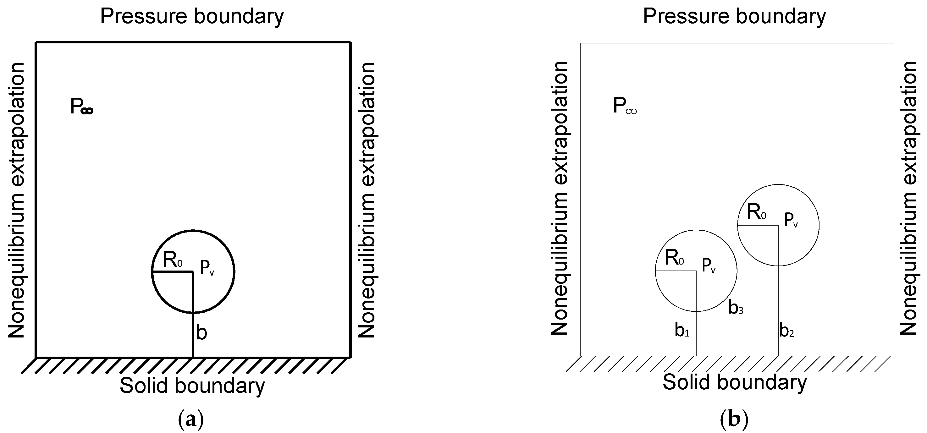
LBM is considered to be one of the most effective methods to solve multiphase flow problems. Commonly used two-dimensional models are D2Q7, D2Q9, etc., where D is the dimension of space and Q is the number of discrete velocities. In this paper, the two-dimensional case is simulated, and in order to ensure the calculation accuracy, nine discrete velocities are used, so the D2Q9 model is used for simulation. The specific arrangement is shown in Figure 1.
In the Boltzmann model, discrete particle distribution function f i is used to replace the fluid particle distribution function:
f i ( x + c e i Δ t , t + Δ t ) = f ( x , t ) 1 τ [ f i ( x , t ) f i e q ( x , y ) ] + F i ( x , t )
where f i ( x , t ) is a single particle density distribution function, f i e q ( x , t ) is the equilibrium particle distribution function, τ is the relaxation time, and the kinematic viscosity is ν = c s 2 ( τ 0.5 ) Δ t . The discrete speed can be defined as
[ e 1 , e 2 , e 3 , e 4 , e 5 , e 6 , e 7 , e 8 , e 9 ] = c [ 0 1 0 0 0 1 0 1 0 1 1 1 1 1 1 1 ] ,
where c = Δ x / Δ t is the grid velocity and Δ x and Δ t are the grid step and time step, respectively. The lattice sound velocity is c s = c / 3 . In the D2Q9 model, the equilibrium distribution function can be expressed as
f i e q ( x , t ) = ω i ρ [ 1 + e i u c s 2 + ( e i u ) 2 2 c s 4 u 2 2 c s 2 ] ,
where u is the fluid velocity and ω i is the weighting factor of the equilibrium distribution function, where ω 1 = 4 / 9 , ω i = 1 / 9 ( i = 2 , 3 , 4 , 5 ) , ω i = 1 / 9 ( i = 6 , 7 , 8 , 9 ) . The discrete velocity weight coefficient is related to the discrete strategy. In the discretized velocity space, the macroscopic velocity and density of the fluid can be expressed as
ρ = i f i ( x , t )
ρ u = i f i ( x , t ) e i .
The single-component multiphase flow interaction force F i ( x , t ) is modelled as follows:
F ( X , t ) = G ψ ( X , t ) i = 2 9 ξ ψ ( X + e i Δ t , t ) e i ,
where G is the interaction strength and ξ i = 1 / 9 ( i = 2 , 3 , 4 , 5 ) , ξ i = 1 / 36 ( i = 6 , 7 , 8 , 9 ) . According to Yuan and Schaefer (2006) [34], the interaction potential can be expressed as ψ = 2 ( p ρ c s ) / G c s 2 , where c s = R T is the lattice sound velocity. Through this interaction potential, different equations of state can be applied.
The C-S state equation can be expressed as follows:
p = ρ R T 1 + b ρ / 4 + ( b ρ / 4 ) 2 ( b ρ / 4 ) 3 ( 1 b ρ / 4 ) 3 a ρ 2 ,
where a = 0.4963 R 2 T c 2 / p c and b = 0.18727 R T c / p c . The critical parameters can be expressed as follows:
T c = 0.3773 a b R
p c = 0.0706 b 2
The forces of the fluid act all over the objects placed in it, and how to integrate these forces into the LBM is very important. An EDM with second-order accuracy is suitable. The Boltzmann equation is discretized in the velocity space, and the term in accordance with the LB equation is derived by the EDM. The external force term in Equation (1) can be expressed as
F i = f i e q ( ρ , u + F Δ t / ρ ) f i e q ( ρ , u ) ,
where F is the total interaction force between the fluid and the solid.

3. Physical Model

In order to obtain the evolution of cavitation bubbles in the near-wall region, the physical models are shown in Figure 2.
The figure above shows the initial layout of the simulation. Here, (a) is the physical model of the study of the evolution of a single cavitation bubble in the near-wall region. R0 is the radius of the cavitation bubble, b is the distance from the centre of the cavitation bubble, Pv is the pressure in the cavitation bubble, and P is the pressure outside the cavitation bubble. The left and right boundaries are infinite areas, the upper boundary is the pressure inlet, and the lower boundary is the rigid wall. (b) is the physical model for the study of the evolution of the double cavitation bubble in the near-wall region. b1 is the distance from the centre of the left cavitation bubble to the rigid wall, b2 is the distance from the centre of the right cavitation bubble to the rigid wall, and b3 is the horizontal distance of the centre of the two cavitation bubbles. The other settings are the same as those of the physical model of a single cavitation bubble in the study of the collapse of the near-wall region.

4. Simulation Content and Parameter Initialization Settings

In this paper, the numerical simulation of cavitation collapse in the near-wall region mainly includes three parts: First, the evolution law of the collapse of a single cavitation bubble in the near-wall region is obtained by numerical simulation, and the bubble deformation is compared with the results of classical experiments to verify the model. Second, the pressure field of the bubble is simulated and theoretically study the mechanism of the erosion of the bubble on the solid sidewall. Third, the previously validated model is used to study the evolution of the double cavitation bubble in the near-wall region. In this paper, if there is no special explanation, the unit in the text always uses the grid unit, the length unit is lu, the time unit is ts, the mass unit is mu, and the temperature unit is tu; thus, the density unit is mu · lu 3 , and the pressure unit is mu · lu 1 ts 2 . The simulated initial layout is the same as the physical model. In the simulation, T/Tc = 0.689 is used to simulate and the equilibrium pressure p = 0.0028 mu · lu 1 ts 2 is gotten by the equal area rule is. In the C-S state of equation, a = 1, b = 4 and R = 1 [34] are adopted. The initial temperature is set to a specific temperature, the velocity is zero, and the density field is initialized as follows:
ρ ( x , y ) = ( ρ l i q u i d + ρ g a s ) / 2 + ( ρ l i q u i d ρ g a s ) / 2 · [ tan h ( ( 2 ( ( x x 1 ) 2 + ( y y 1 ) 2 R 0 ) / W ) ] ,
where x1 and y1 is the location of the middle of the bubble at the initial moment, the hyperbolic tangent function t a n h = ( e x e x ) / ( e x + e x ) and the phase interface width is W = 4. Since the cavitation bubble radius is approximately ten times the width of the phase interface, it can obtain better numerical stability of the model, but it is essential to ensure that the bubble collapse is not affected by other boundaries and that the calculation cost is reduced. Therefore, our simulation calculation area is 401 × 401.
Through the C-S state equation, the P‒V curve of the gas‒liquid isotherm curve can be obtained, and then the Maxwell construction should be used, which can be stated as
V m , l V m , g P d V m = p 0 ( V m , g V m , l ) ,
where P is the pressure in the EOS and p 0 is a constant pressure. When the equation is established, p 0 is the equilibrium pressure, and Vm,g and Vm,l are the physical quantities that characterize the equilibrium gas pressure and the equilibrium liquid pressure, respectively. In addition, the coexistence densities ρ v and ρ l of gas and liquid, respectively, can also be determined by phase separation simulation with a slight random disturbance of the initial density. In the calculation process, ρ l need to be slightly adjusted to ensure ρ l has the same density as the pressure boundary so that an additional pressure difference between the inside and the outside of the bubble is obtained after the fluid balance in the entire calculation domain.
The collapse of cavitation bubbles under the influence of a single wall surface is studied, so infinite areas are needed on both the left and right sides to ensure the computing domain is unaffected by the boundary fluctuations. Under the premise of the minimum calculation area, the unbalanced extrapolation format is well suited for our needs. Therefore, the non-equilibrium extrapolation format is used for the left and right borders. The bottom boundary uses a standard bounce-back format. In addition, a pressure boundary condition is applied at the inlet, and the liquid pressure in the calculation zone is equal to the pressure boundary pressure.

5. Study of the Evolution of a Single Cavitation Bubble

Detailed experimental data have been obtained for the evolution of cavitation bubble collapse at different distances from the wall [35]. However, traditional experimental data and numerical simulation have great limitations. For example: Plesset and Chapman [36] made six assumptions, including negligible surface tension, constant vapour pressure and ambient pressure, an incompressible liquid, non-viscous flow, and no permanent gas, which are challenging to satisfy in experiments and LBM simulations, resulting in inapplicability to specific practical problems. In this paper, using the improved Shan‒Chen model, numerical simulation data of cavitation bubble collapse at different locations are obtained at a specific temperature. This part of the study mainly consists of two parts: the first part verifies the simulation results by comparison with physical experiments, and the second part obtains the evolution law of the collapse of a single cavitation bubble in detail. The following is a comparative analysis of density field images of LBM numerical simulations and experimental images of cavitation bubbles collapsing at two different positions with the same radius and pressure. Through comparison with the experimental data of Philipp [35], the LBM calculation results which are shown in Figure 3 and Figure 4 are found to be consistent with the qualitative analysis of the experimental data which are shown in Figure 5 and Figure 6.
Figure 3 shows the change of density field during the collapse of cavitation bubbles. In this simulation, a dimensionless quantity λ = b/R0 was introduced, which is the amount that characterizes the distance from the centre of the bubble to the wall. The figures below show cases with λ = 1.6, R 0 = 80 lu and λ = 2.5, R 0 = 80 lu. The cavitation bubble is initially a circle. The bubble size and the thickness of the gas‒liquid boundary layer are controlled by Equation (11). Since the pressure difference exists inside and outside the bubble, the bubble is deformed by extrusion. Due to the influence of the bottom rigid sidewall, the longitudinal flow is blocked, and a negative pressure forms under the bubble to induce longitudinal expansion of the bubble. Due to the shrinkage and deformation of the bubbles, the volume is decreasing, and the surrounding liquid fills the space created by the bubbles, resulting in a decrease in the density and pressure around them. Then, the pressure of the upper pressure boundary is first transmitted to the upper surface of the bubble, and a high-pressure zone is formed in the upper part of the bubble that acts together with the low-pressure zone of the cavitation bubble to form a depression at the upper portion (t = 470). Due to the rebound effect of the liquid and the relatively high speed of movement of the upper portion of the bubble, a relatively large conical high-pressure region is formed in the upper portion, which is crucial in the subsequent deformation. Over time, the depression continues to expand (t = 530), and with the influence of the surrounding high pressure, the bubble gradually shrinks, assuming a crescent shape (t = 570). When the sag causes the upper surface of the bubble to touch the lower surface, a large pressure difference directly breaks down the empty bubble, forming a micro shock wave, which has a destructive effect on the wall surface (t = 588). At the same time, a complex sound field is generated, which causes additional damage to the rigid wall. By comparison, the morphology of cavitation bubble collapse differs for different dimensionless parameters λ and ΔP is confirmed. In our simulation, a crescent-shaped bubble is formed at λ = 1.6 and is then broken down to form two bubbles, which generates a micro-shock; however, at λ = 2.5, the bubble is squashed directly. A crescent-shaped bubble is formed, but the bubble does not break in the middle and finally collapses in the form of a small bubble. The calculation results are consistent with the results of Philipp [35]. When the bubble is too far from the wall surface, the sidewall has a small retarding effect on the bubble, and a strong negative pressure is unlikely to form under the bubble, so when the bubble collapses, the bubbles are gradually crushed and collapsed, and the impact of the formed pressure on the wall surface is also alleviated.

6. Study of the Evolution of a Double Cavitation Bubble

In the previous section, the collapse evolution of a single cavitation bubble in the near-wall region was discussed, which was found to be in good agreement with the physical experiment, thus verifying the stability of the numerical simulation model. However, in actual engineering, cavitation bubbles do not appear alone. Cavitation clouds typically form in cavitation-concentrated areas, and hundreds of cavitation bubbles interact and collapse under the extra pressure; thus, the erosion of the wall is more complex. This research area merits further study and is instructive for the possibility of reducing cavitation damage. In our study, using the previously validated mathematical model, the collapse evolution law by simulating the collapse of two cavitation bubbles in the near-wall region under pressure induction was obtained. Taking two of these cases as examples, the evolution of the two cavitation bubbles in the near-wall region under pressure induction was analysed. For convenience of description, the left and right bubbles are designated left bubble (LB) and right bubble (RB), respectively. The spatial direction is set as shown in Figure 1. For example, the upper right is the e6 direction. Similar to the previous simulation, the dimensionless quantities λ1, λ2, and λ3 is introduced, where λ1 = b1/R0, which is the amount that characterizes the distance of the LB centre from the wall; λ2 = b2/R0, which is the amount that characterizes the distance of the LB centre from the wall surface; and λ3 = b3/R0, which is the amount that represents the horizontal distance between the LB and RB centres.

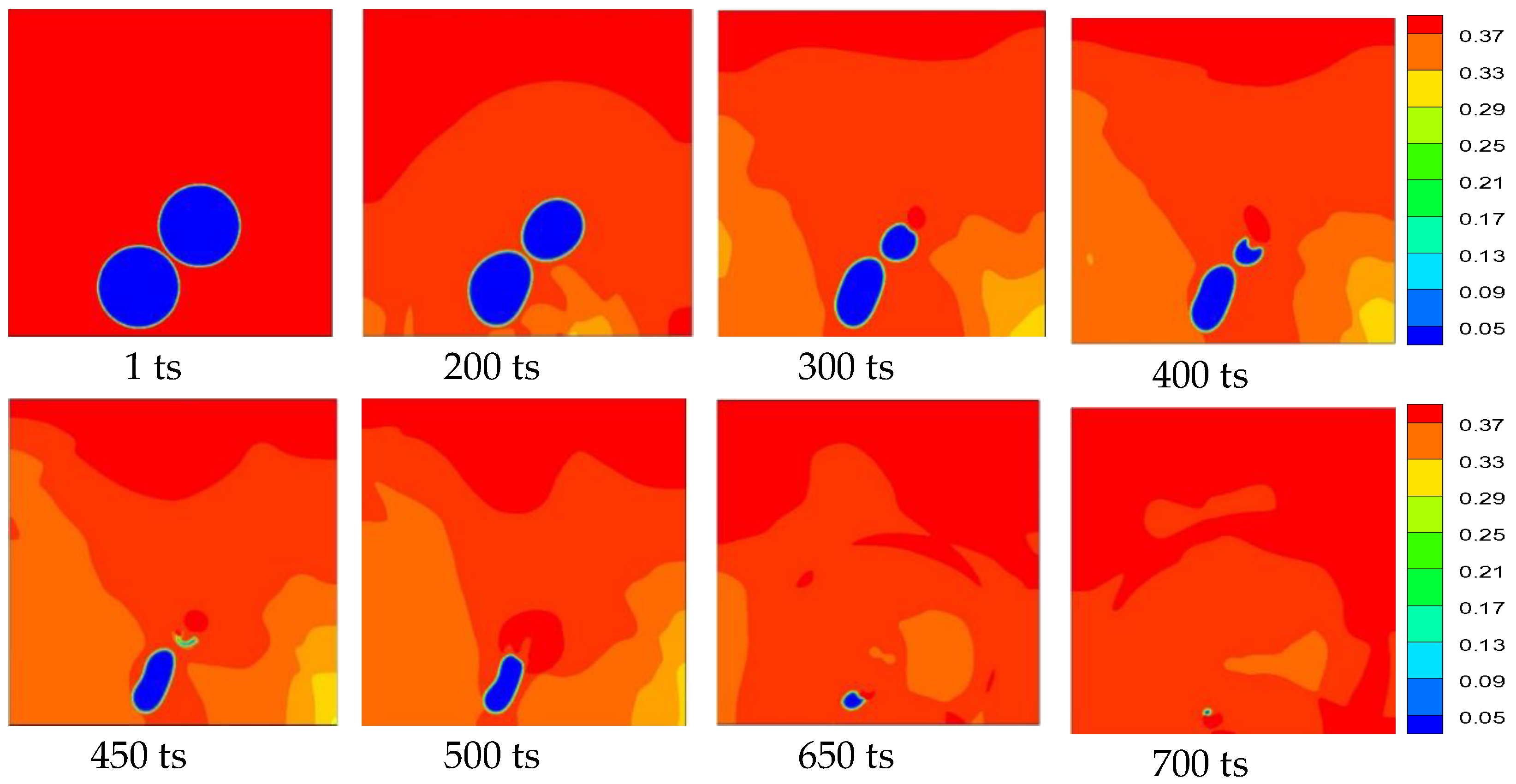
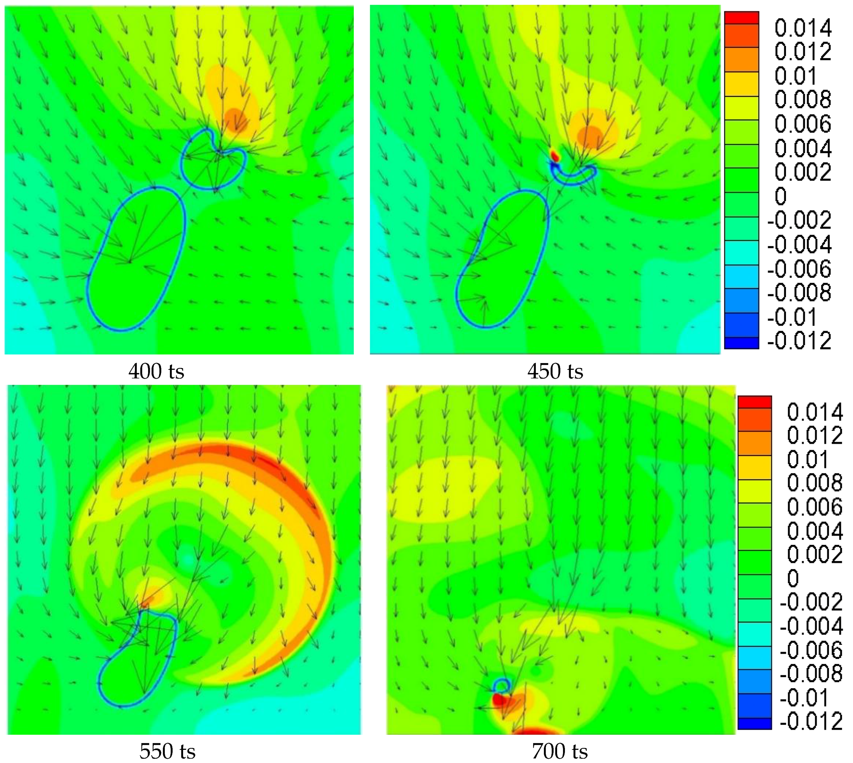
6.1. Case 1: Numerical Simulation of Tilt Distribution Cavitation with Two Cavitation Bubbles

When λ1 = 1.2, λ2 = 2.7, and λ3 = 1.5, the line connecting the centres of the two cavitation bubbles is at an angle of 45° to the wall surface. The density field and the pressure field coupling with the velocity field of the cavitation bubble collapse process are shown in Figure 7 and Figure 8, respectively.
The cavitation bubble distribution at the initial moment is as shown by t = 1 ts, and the specific parameter settings are the same as the previous settings. The collapse process of each cavitation bubble was analysed. When the simulation proceeds to t = 200 ts, the change of LB is similar to the collapse of a single cavitation bubble. Due to the blockage of the wall surface, a low-pressure zone is formed in the bottom region, and LB exhibits an elongated deformation state in the e5 direction. The e6 direction of the LB and the e8 direction of the RB are attracted to each other, and the opposite direction is deformed. If the gas density and the liquid density are in equilibrium at this time, the two cavitation bubbles would attract each other and eventually merge into a single bubble. However, since the liquid has been pressurized during the simulated initialization, the additional generated pressure prevents the emergence of the two bubbles. As the simulation progresses, the deformation is further aggravated, and the bubbles decrease under the action of additional pressure. Between them, the change of LB is the most easily detected. When the time reaches t = 350 ts, the LB is elongated and deformed due to the low pressure resulting from the blockage of the wall surface; the e6 direction of RB appears the same as the change of a single cavitation bubble in the near-wall region, and a depression occurs. The change becomes more apparent at 400 ts. Around the shrinking bubble, the liquid fills the newly available space, and a slightly lower pressure appears around the cavitation bubble. The transition can be observed in the velocity field. Around the bubble, the velocity direction tends to support cavitation. Note that in the figure of the pressure field and the velocity field, for the sake of convenience, only the velocity of the liquid is shown and we do not plot the velocity inside the bubble. The LB exhibits an elliptical shape that exhibits an inclination in the e6–e8 direction under the action of the sidewall, the attraction of RB and the external extreme pressure. The RB is also elliptical due to the attraction of the two bubbles, but the deformation is not as strong as with the bubble on the left. At this time, relative with the collapse rule of a single cavitation bubble in the near-wall region, LB is equivalent to rigidity avoidance for RB, so a low-pressure zone is generated between the two bubbles, and high pressure is generated by the upper pressure boundary. A pressure difference is generated in the e6–e8 direction of the RB caused the deformation to continue to produce. Inspection of the velocity field reveals that the maximum velocity occurs in the same direction of the RB. At t = 450 ts, the cavitation bubble is crescent-shaped. The bubble is strongly compressed from the upper part of the depression until the entire bubble is completely collapsed from the upper part of the bubble, which occurs because the flow field is not completely symmetrical on both sides of the e6–e8 direction. The upper part is first crushed by the pressure transferred from the pressure boundary. The other reason is that the most attractive part of LB is located at the nearest position of the two bubbles. The velocity field indicates that the maximum velocity direction has been deflected, and RB begins to collapse from top to bottom under the pressure difference, producing a huge jet and complex sound field. The huge pressure generated by the collapse acts in conjunction with other factors to promote the continued collapse of LB. At t = 550 ts, the pressure field and velocity field images indicate that the flow field changes due to the collapse pressure of RB, and the micro-jet generated by RB in the e6 direction collides with the downward flowing liquid to generate a high voltage and noise, and energy begins to be consumed; furthermore, the micro-jet in the e7 direction overlaps with the original flow field, and the flow state becomes complex. As the simulation proceeds, the flow field exhibits vortices, and LB begins to collapse. First, the cavitation bubble e6 direction begins to shrink under the influence of the pressure of RB, which causes a protrusion in the upper portion of the cavitation bubble. At this time, the energy generated by the RB collapse is insufficient to continue to compress LB. Under the joint action of the upper pressure boundary pressure and the high pressure generated by the RB collapse, a high-pressure region (t = 550 ts) is formed at the upper convex portion, and collapse from the upper portion of the cavitation bubble is induced. As RB is destroyed, the e9 direction finally collapses, and a jet from the e7 to the e9 direction is generated in the flow field, so that the entire flow field exhibits vortices. Finally, LB collapses under the combined action of various factors, and the generated pressure impacts the wall surface to avoid impact. The pressure field diagram of t = 700 ts indicates that a high pressure is generated on the wall surface. Note that after RB collapse, LB collapse occurs under the influence of various factors, and the mechanism of action is relatively complex. The LB high-pressure zone rotates around the cavitation bubble. This visualization is a powerful way to illustrate the complex vortices and other phenomena in the flow field, involving other physical quantities. The parameters of this study cannot describe the more detailed characteristics. The specific mechanism needs further study.

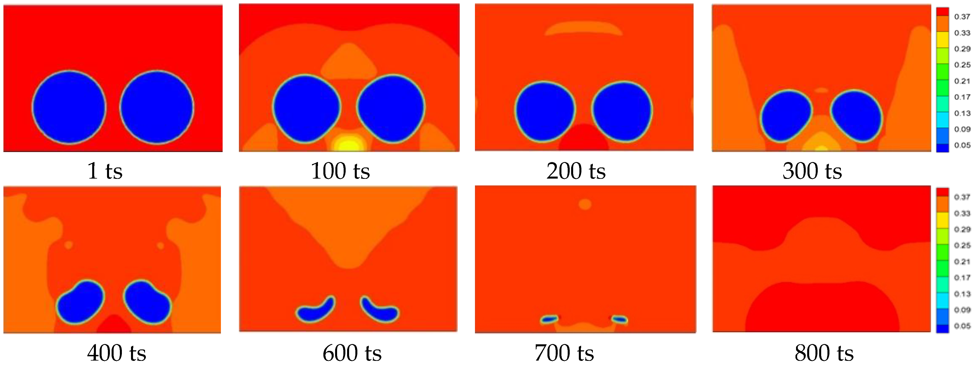
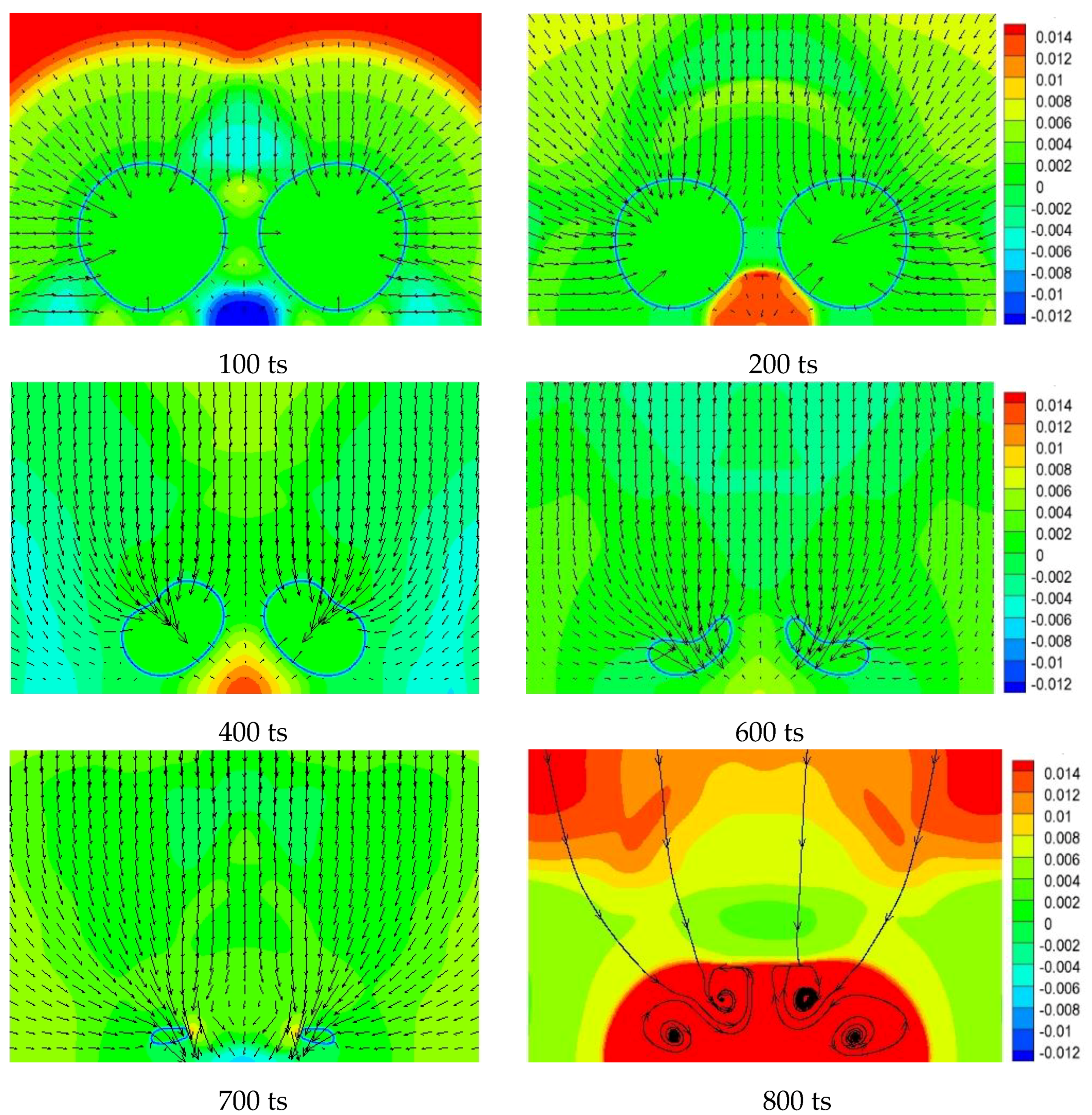
6.2. Case 2: Numerical Simulation of Two Parallel Cavitation Bubbles

When λ1 = 1.2, λ2 = 1.2, and λ3 = 2.4, that is, the line connecting the centres of the two cavitation bubbles is parallel to the wall surface, and the density field of the cavitation bubble collapse process is shown in Figure 9 as well as the pressure field and the velocity field shown in Figure 10.
The figure shows the change in the two cavitation bubbles in the near-wall region and the initial boundary and density settings are the same as described above. Since the changes of the two bubbles are basically the same, the LB is used as an example for analysis. At t = 100 ts, low pressure is created at the bottom of the cavitation bubbles due to the retardation of the rigid wall. At the same time, the two cavitation bubbles are attracted to each other. The cavitation bubbles that are not attracted to the rigid wall and the cavitation bubbles begin to shrink under the action of the additional pressure, and the new space that is generated from the reduced area was filled by the surrounding liquid. Through the analysis of the pressure field, the conclusion that the pressure decreases in the e 9 direction of LB can be obtained. The bottom region of the symmetry axis is defined as the pressure change region, which is the region where the pressure change is most obvious during the cavitation process, except for the pressure region generated by the collapse of the cavitation bubble itself. In the simulation, under the condition of the specific additional pressure and the relative position of the cavitation bubble, a new cavitation bubble is generated in the pressure change zone, but it will collapse quickly. Although the new cavitation bubbles are produced for a short period of time, the effect on the flow field is very important and will be explained in detail in the analysis of the maximum wall pressure behind. When the simulation is carried out to t = 200 ts, for LB, the high pressure generated by the collapse of the new cavitation bubble in the pressure change zone continues to act on the e 9 direction of the cavitation bubble, showing a slightly lifted shape. As the simulation progresses to t = 400 ts, the deformation continues; the deformation of the cavitation bubbles is already evident, and the cavitation bubbles are inclined at an inclination angle of 45°, and the cavitation bubbles become crescent-shaped. This is mainly due to the interaction between the cavitation bubbles, the interaction between the cavitation bubbles and the wall surface, and the collapse of the new cavitation bubbles in the pressure change zone. In addition, the velocity field indicates that the velocity of the LB in the e 7 direction is the largest. At t = 600 ts, the LB appears asymmetric on the axis in the e 7 e 9 direction. The upper part is strongly influenced by the pressure boundary and the lower part is strongly influenced by the rigid wall. Therefore, the position where the pressure difference between the upper side and the lower side of the LB is the largest is located at the centre, so that the cavitation bubbles collapse from the upper portion until they completely collapse. For each bubble, a complex eddy current phenomenon occurs in the flow field because the collapse does not occur instantaneously but spreads from the top to the adjacent region. The 800 ts streamline diagram clearly shows the eddy currents in the flow.

7. Maximum Wall Pressure

The maximum wall pressure of a single cavitation bubble and two parallel distributed cavitation bubbles collapsed in the near-wall region was identified in this study. The initial conditions are set as follows: For the case of a single cavitation bubble, the value of λ (from 1.05–2.0) with a series of gradients is used to simulate the maximum wall pressure resulting from single cavitation bubble collapse under different initial conditions. Since the maximum pressure of a single cavitation bubble on the wall is only likely to occur below the cavitation bubble ( e 5 direction), the pressure of the wall below the cavitation bubble is recorded to find the maximum value. For the case of a single cavitation bubble, a lambda value (from 1.05–2.0) with a series of gradients is used to simulate the maximum wall pressure resulting from a single cavitation bubble collapse under different initial conditions. Since the maximum pressure of a single cavitation bubble on the wall is only likely to occur below the cavitation bubble ( e 5 direction), the pressure of the wall below the cavitation bubble is recorded to find the maximum value. For the case of two cavitation bubbles, λ3 = 2.4 is used and, likewise, the value of λ (from 1.05 to 2.0) with a series of gradients was used to simulate the maximum wall pressure resulting from the collapse of two cavitation bubbles under different initial conditions, where λ = λ1 = λ2. Since the cavitation bubble collapse process is complicated, the maximum wall pressure is not generated at the same position for the collapse process under different initial conditions. The wall pressure below the cavitation bubble ( e 5 direction) and the pressure change zone is recorded to find the maximum value The comparison of the maximum wall pressure under different initial conditions is shown in Figure 11.
Some conclusions are given by analysis:
  • The maximum wall pressure generated by the collapse of a single cavitation bubble in the near-wall region decreases with increasing distance from the wall surface, and it first drops sharply, then slowly decreases and finally becomes relatively stable. This is because the closer to the wall, the smaller the thickness of the fluid that the micro shock wave generated by cavitation passes to the wall and the smaller the blockage effect of the flow field, the greater the wall pressure generated.
  • It is complex for the case where a double parallel cavitation bubble collapses in the near-wall region because the maximum wall pressure produces a different position under different initial conditions. When λ = 1.05–1.10, the wall below the cavitation bubble is subjected to the maximum wall pressure, because the cavitation bubble is closer to the wall surface, and the generated micro-shock is transmitted to the wall surface almost unimpeded and the cavitation bubble of the pressure change region is not fully developed, which is not enough to generate create a huge pressure with the lifting force to bubble. When λ = 1.15–1.25, the maximum wall pressure occurs in the pressure change zone where new cavitation bubbles are generated and collapse rapidly, resulting in a large wall pressure exceeding the maximum wall pressure at other locations. When λ = 1.40–2.0, the area where the maximum wall pressure is generated is the pressure change zone, but the pressure generation at this time is not when the new cavitation bubble collapses but the pressure after the collapse of the two cavitation bubbles overlaps each other on the wall. The change in wall pressure depends mainly on the size of the new cavitation bubble induced and the pressure generated by the collapse and the lifting force of the bubbles.
  • When λ < 1.7, the wall pressure generated by the collapse of a single cavitation bubble is relatively large. This is because, for the case where the double cavitation bubble collapses in the near-wall region, the pressure generated by the collapse of the new cavitation bubble induced in the pressure change region has an effect of lifting force on the cavitation bubble. Thereby, the bottom pressure of the cavitation bubble collapse is increased, and the blockage effect of the wall surface is weakened, which is equivalent to an increase of λ, and the resulting wall pressure is relatively small. When λ > 1.7, the wall pressure of the pressure change zone is formed by the superposition of pressure generated by the collapse of two cavitation bubbles, so the generated wall pressure is greater than the pressure generated by the collapse of a single cavitation bubble.
In summary, the maximum wall pressure generated by the collapse of the two cavitation bubbles in the near-wall region is smaller than the single cavitation bubble at λ < 1.7; the closer the bubble is to the wall, the greater the influence on the wall surface. When λ > 1.7, the distance between the cavitation bubble pair and the wall surface has little effect on the maximum wall pressure. This is a point worthy of further study with different initial conditions. It can be used as a reference for reducing cavitation damage in practical engineering.

8. Conclusions

Based on the improved lattice Boltzmann Shan‒Chen model coupled with C-S EOS, the collapse phenomenon of cavitation bubbles in the near-wall region is studied. In this paper, the collapse of a single bubble in the near-wall region is simulated and compared with the physical experiment; the results are in good agreement. Then, using the verified mathematical model, the simulation of the collapse of two cavitation bubbles in the near-wall region under different pressure-induced conditions is carried out, and the collapse evolution law is obtained. And analysed the effect of wall pressure on different initial conditions. By analysing in detail the density field changes and pressure field changes during bubble collapse, the following conclusions can be drawn:
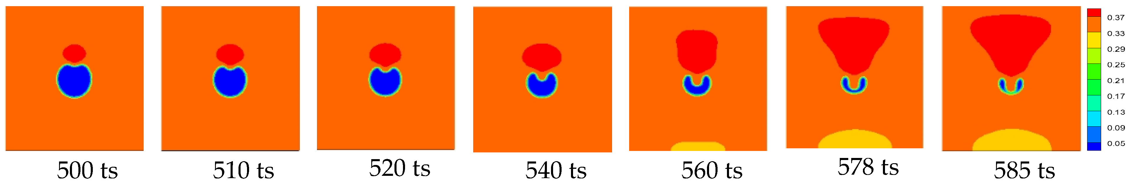
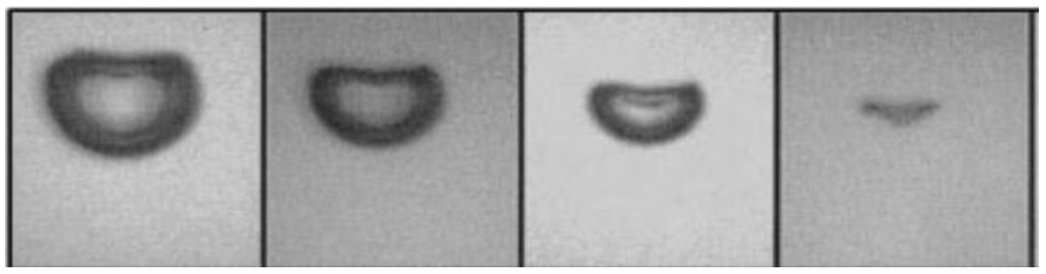
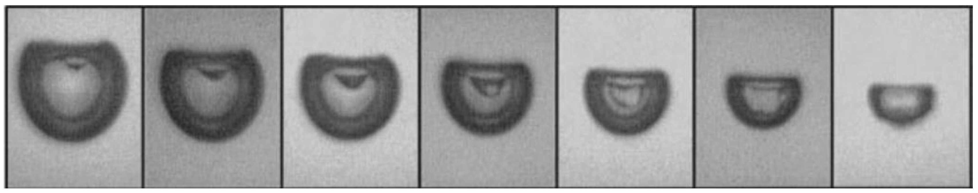
  • For the case where a single cavitation bubble collapses in the near-wall region, when λ = 1.6, a crescent-shaped bubble is formed that is broken down to form two bubbles, and a micro-shock is generated; when λ = 2.5, the bubbles are crushed to form crescent-shaped bubbles, but the bubbles do not break in the middle but rather ultimately collapse in the form of a small bubble. The shape of the cavitation bubble is related to the distance of the cavitation bubble from the rigid wall.
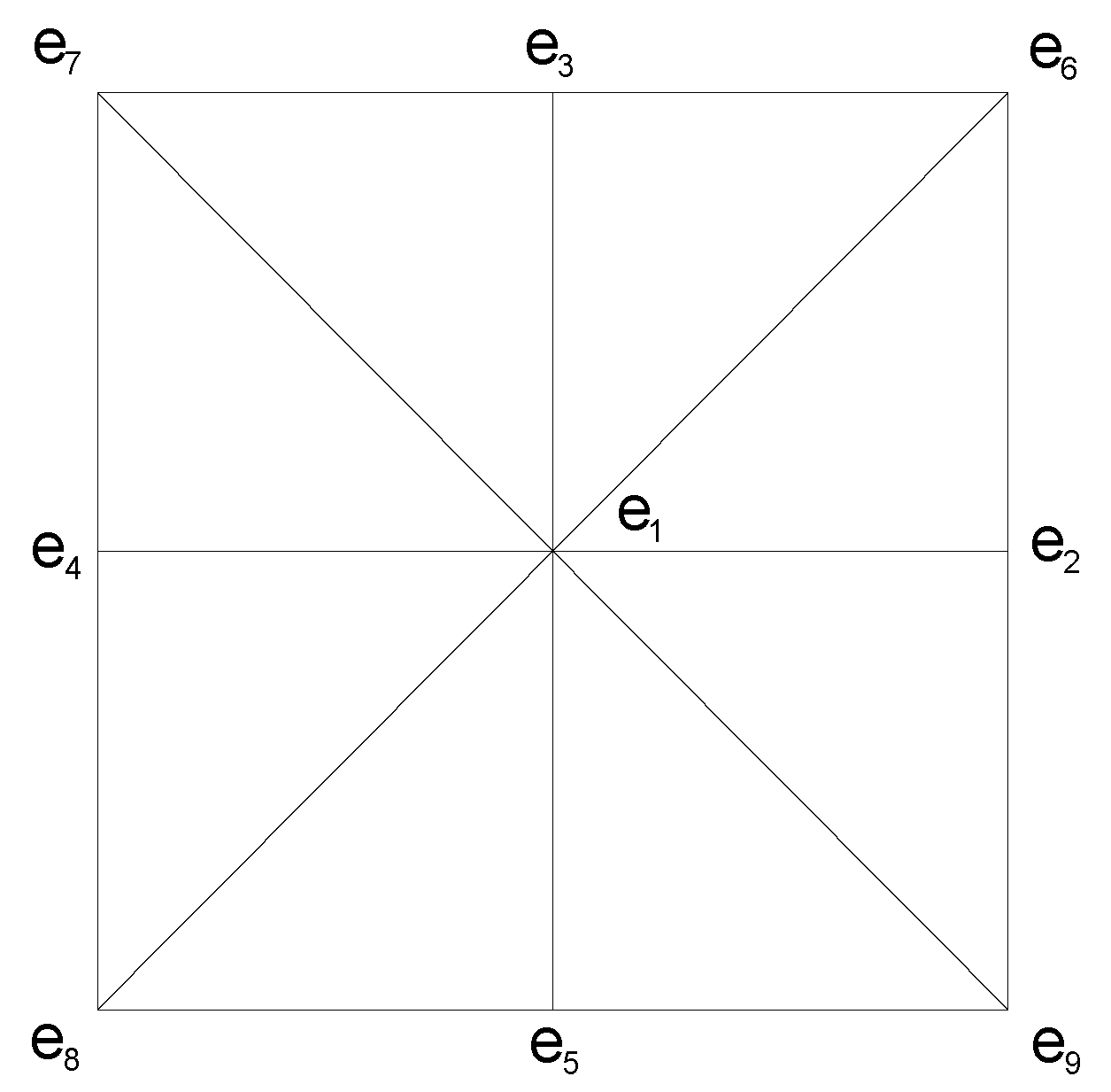
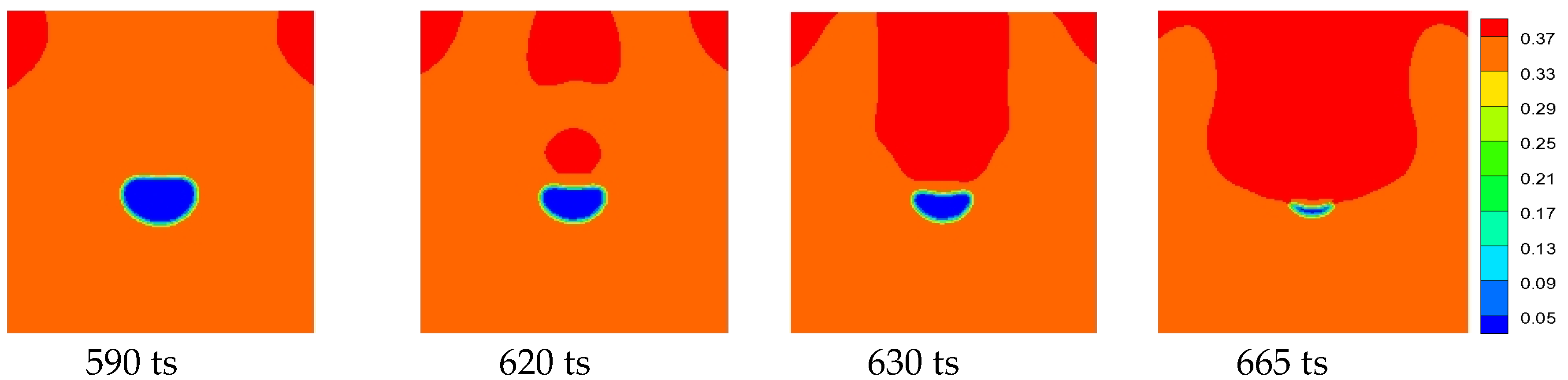
  • For the numerical simulation of tilted distribution cavitation with two cavitation bubbles, in the early stage of simulation, the collapse behaviour is similar to that of the single-bubble case. Subsequently, the e6 direction of RB has a concave deformation, which is very important in the collapse of the two bubbles. The velocity field indicates that the maximum velocity appears in the depression of RB. The tremendous pressure generated by this velocity directly penetrates the bubble; thereafter, the bubble is crescent-shaped until collapsing completely. Due to the asymmetry of the collapse, the flow field becomes complex after RB collapses and particularly so after LB collapses, and vortices appear in the flow field.
  • For the numerical simulation of parallel distribution cavitation of two bubbles, the bubble collapses under the blocking effect of the rigid wall and the attraction of the two bubbles, and the two bubbles collapse simultaneously. Therefore, the mutual influence during the collapse process is smaller than that of Case 1; in addition, the erosion effect of the bubble collapse on the wall surface is the result of superimposing the pressure fields formed by the collapse of the two bubbles. However, for each bubble, since the collapse does not occur instantaneously but is collapsed from the upper part of the closest position of the two cavitation bubbles, a complex vortex phenomenon occurs in the flow field.
  • By comparing the maximum wall pressure generated by cavitation under different initial conditions, the factors affecting the maximum wall pressure are obtained. For a single cavitation bubble, the distance from the wall is the most important factor. For two cavitation bubbles, the lifting effect of the new induced cavitation bubble collapse is the most important factor.
The results indicate that the improved LBM Shan‒Chen model has many advantages in simulating cavitation problems, providing a reference for further simulation.
All the abbreviations are explained in the Appendix A (Table A1).

Author Contributions

Conceptualization, Y.P. and J.Z.; Methodology, Y.P. and J.Z.; Software, Y.M.; Investigation, Y.M.; Data Curation, Y.M.; Writing-Original Draft Preparation, Y.P. and J.Z.; Writing-Review & Editing, Y.M.; Visualization, Y.M.; Funding Acquisition, Y.P.

Funding

This research was funded by the National Natural Science Foundation of China (51579166) and the National Key Research and Development Program of China (2016YFC0401705).

Conflicts of Interest

The authors declare no conflict of interest.

Appendix A

Table A1. All variables with definitions.
f i Single Particle Density Distribution Function
f i e q equilibrium particle distribution function
τ relaxation time
ν kinematic viscosity
c grid velocity
Δ x grid step
Δ t time step
c s lattice sound velocity
ω i weighting factor
ufluid velocity
F i interaction force
ψ interaction potential
T c critical temperature
P c critical pressure
Ftotal interaction force
Pvpressure of the cavitation bubble
Pthe pressure outside the cavitation bubble
R0radius of the cavitation bubble
b ( b 1 , b 2 , b 3 )distance between corresponding points
Tlattice temperature
a (in Equation (11))parameter of the C-S state of equation
b (in Equation (11))parameter of the C-S state of equation
R (in Equation (11))parameter of the C-S state of equation
V m , g the equilibrium gas pressure
V m , l the equilibrium liquid pressure
λ( λ 1 , λ 2 , λ 3 )dimensionless value that characterizes the distance

References

  1. Kling, C.L.; Hammitt, F.G. A photographic study of spark-induced cavitation bubble collapse. J. Basic Eng. 1972, 94, 825–832. [Google Scholar] [CrossRef]
  2. Lauterborn, W. High-speed photography of laser-induced breakdown in liquids. Appl. Phys. Lett. 1977, 31, 663–664. [Google Scholar] [CrossRef]
  3. Lauterborn, W.; Bolle, H. Experimental investigations of cavitation-bubble collapse in the neighbourhood of a solid boundary. J. Fluid Mech. 1975, 72, 391–399. [Google Scholar] [CrossRef]
  4. Reuter, F. Electrochemical wall shear rate microscopy of collapsing bubbles. Phys. Rev. Fluids 2018, 3, 063601. [Google Scholar] [CrossRef]
  5. Watanabe, R.; Yanagisawa, K.; Yamagata, T.; Fujisawa, N. Simultaneous shadowgraph imaging and acceleration pulse measurement of cavitating jet. Wear 2016, 358–359, 72–79. [Google Scholar] [CrossRef]
  6. Reuter, F.; Cairos, C.; Mettin, R. Vortex dynamics of collapsing bubbles: Impact on the boundary layer measured by chronoamperometry. Ultrason. Sonochem. 2016, 33, 170–181. [Google Scholar] [CrossRef] [PubMed]
  7. Cui, P.; Zhang, A.M.; Wang, S.P.; Khoo, B.C. Ice breaking by a collapsing bubble. J. Fluid Mech. 2018, 841, 287–309. [Google Scholar] [CrossRef]
  8. Rossello, J.M.; Urteaga, R.; Bonetto, F.J. A novel water hammer device designed to produce controlled bubble collapses. Exp. Therm. Fluid Sci. 2018, 92, 46–55. [Google Scholar] [CrossRef]
  9. Pal, A.; Joseph, E.; Vadakkumbatt, V.; Yadav, N.; Srinivasan, V.; Maris, H.J.; Ghosh, A. Collapse of Vapor-Filled Bubbles in Liquid Helium. J. Low Temp. Phys. 2017, 188, 101–111. [Google Scholar] [CrossRef]
  10. Daou, M.M.; Igualada, E.; Dutilleul, H.; Citerne, J.-M.; Rodriguez-Rodriguez, J.; Zaleski, S.; Fuster, D. Investigation of the collapse of bubbles after the impact of a piston on a liquid free surface. AIChE J. 2017, 63, 2483–2495. [Google Scholar] [CrossRef] [Green Version]
  11. Ma, X.J.; Huang, B.A.; Zhao, X.; Wang, Y.; Chang, Q.; Qui, S.; Fu, X.; Wang, G. Comparisons of spark-charge bubble dynamics near the elastic and rigid boundaries. Ultrason. Sonochem. 2018, 43, 80–90. [Google Scholar] [CrossRef] [PubMed]
  12. Gong, S.W.; Ohl, S.W.; Klaseboer, E.; Khoo, B.C. Interaction of a spark-generated bubble with a two-layered composite beam. J. Fluids Struct. 2018, 76, 336–348. [Google Scholar] [CrossRef]
  13. Oh, J.; Yoo, Y.; Seung, S.; Kwak, H.-Y. Laser-induced bubble formation on a micro gold particle levitated in water under ultrasonic field. Exp. Therm. Fluid Sci. 2018, 93, 285–291. [Google Scholar] [CrossRef]
  14. Sukop, M.C.; Or, D. Lattice Boltzmann method for homogeneous and heterogeneous cavitation. Phys. Rev. E 2005, 71. [Google Scholar] [CrossRef] [PubMed]
  15. Chen, X.P.; Zhong, C.W.; Yuan, X.L. Lattice Boltzmann simulation of cavitating bubble growth with large density ratio. Comput. Math. Appli. 2012, 61, 3577–3584. [Google Scholar] [CrossRef]
  16. Shan, M.L.; Zhu, C.P.; Zhou, X.; Yin, C.; Han, Q.B. Investigation of cavitation bubble collapse near rigid boundary by lattice Boltzmann method. J. Hydrodyn. 2016, 28, 442–450. [Google Scholar] [CrossRef]
  17. Zhou, X.; Shan, M.L.; Zhu, C.P.; Chen, B.Y.; Yin, C.; Ren, Q.G.; Han, Q.B.; Tang, Y.B. Simulation of Acoustic Cavitation Bubble Motion by Lattice Boltzmann Method. Appl. Mech. Mater. 2014, 580–583, 3098–3105. [Google Scholar] [CrossRef]
  18. Kucera, A.; Blake, J.R. Approximate methods for modeling cavitation bubbles near boundaries. Bull. Austral. Math. Soc. 1990, 41, 1–44. [Google Scholar] [CrossRef]
  19. Li, B.B.; Zhang, H.C.; Han, B.; Chen, J.; Ni, X.W.; Lu, J. Investigation of the collapse of laser-induced bubble near a cone boundary. Acta Phys. Sin. 2012, 61, 21. [Google Scholar]
  20. Zhang, X.M.; Zhou, C.Y.; Islam, S.; Liu, J.Q. Three-dimensional cavitation simulation using lattice Boltzmann method. Acta Phys. Sin. 2009, 58, 8406–8414. [Google Scholar]
  21. Mishra, S.K.; Deymier, P.A.; Muralidharan, K.; Frantziskonis, G.; Pannala, S.; Simunovic, S. Modeling the coupling of reaction kinetics and hydrodynamics in a collapsing cavity. Ultrason. Sonochem. 2010, 17, 258–265. [Google Scholar] [CrossRef] [PubMed]
  22. Schanz, D.; Metten, B.; Kurz, T.; Lauterborn, W. Molecular dynamics simulations of cavitation bubble collapse and sonoluminescence. New J. Phys. 2012, 14. [Google Scholar] [CrossRef]
  23. Du, T.; Wang, Y.; Huang, C.; Liao, L. A numerical model for cloud cavitation based on bubble cluster. Theor. Appl. Mech. Lett. 2017, 7, 231–234. [Google Scholar] [CrossRef]
  24. Wang, Q.; Yao, W.; Quan, X.; Cheng, P. Validation of a dynamic model for vapor bubble growth and collapse under microgravity conditions. Int. Commun. Heat Mass Transf. 2018, 95, 63–73. [Google Scholar] [CrossRef]
  25. Ogloblina, D.; Schmidt, S.J.; Adams, N.A. Simulation and analysis of collapsing vapor-bubble clusters with special emphasis on potentially erosive impact loads at walls. EPJ Web Conf. 2018, 180, 9. [Google Scholar] [CrossRef]
  26. Chen, Y.; Lu, C.J.; Chen, X.; Li, J.; Gong, Z.X. Numerical investigation of the time-resolved bubble cluster dynamics by using the interface capturing method of multiphase flow approach. J. Hydrodynam. 2017, 29, 485–494. [Google Scholar] [CrossRef]
  27. Ming, L.; Zhi, N.; Chunhua, S. Numerical Simulation of Cavitation Bubble Collapse within a Droplet. Comput. Fluids 2017, 152, 157–163. [Google Scholar] [CrossRef]
  28. Peng, K.; Tian, S.; Li, G.; Huang, Z.; Yang, R.; Guo, Z. Bubble dynamics characteristics and influencing factors on the cavitation collapse intensity for self-resonating cavitating jets. Petrol. Explor. Dev. 2018, 45, 343–350. [Google Scholar] [CrossRef]
  29. Xue, H.H.; Shan, F.; Guo, X.S.; Tu, J.; Zhang, D. Cavitation Bubble Collapse near a Curved Wall by the Multiple-Relaxation-Time Shan-Chen Lattice Boltzmann Model. Chin. Phys. Lett. 2017, 34, 83–87. [Google Scholar] [CrossRef]
  30. Tagawa, Y.; Peters, I.R. Bubble Collapse and Jet Formation in Corner Geometries. Phys. Rev. Fluids 2018, 2. [Google Scholar] [CrossRef]
  31. Goncalves, E.; Zeidan, D. Numerical study of bubble collapse near a wall. AIP Conf. Proc. 2018, 1978. [Google Scholar] [CrossRef]
  32. Peng, Y.; Mao, Y.F.; Wang, B. Study on C–S and P–R EOS in pseudo-potential lattice Boltzmann model for two-phase flows. Int. J. Mod. Phys. C 2017, 28. [Google Scholar] [CrossRef]
  33. Peng, Y.; Wang, B.; Mao, Y. Study on Force Schemes in Pseudopotential Lattice Boltzmann Model for Two-Phase Flows. Math. Probl. Eng. 2018. [Google Scholar] [CrossRef]
  34. Yuan, P.; Schaefer, L. Equations of state in a lattice Boltzmann model. Phys. Fluids 2006, 18. [Google Scholar] [CrossRef]
  35. Philipp, A.; Lauterborn, W. Cavitation erosion by single laser-produced bubbles. J. Fluid Mech. 2000, 361, 75–116. [Google Scholar] [CrossRef]
  36. Plesset, M.S.; Chapman, R.B. Collapse of an initially spherical vapour cavity in the neighbourhood of a solid boundary. J. Fluid Mech. 1970, 47, 283–290. [Google Scholar] [CrossRef]
Figure 1. D2Q9 model.
Water 10 01439 g001
Figure 2. Physical model. (a) (single bubble model); (b) (double bubbles model) (R0—bubble initial radius; bi—distance; Pv—vapour pressure in bubble; P—ambient pressure).
Water 10 01439 g002
Figure 3. Density field of the LBM simulation: λ = 2.5, R 0 = 80 lu.
Water 10 01439 g003
Figure 4. Density field of the LBM simulation: λ = 1.6, R 0 = 80 lu.
Water 10 01439 g004
Figure 5. Experimental images: λ = 2.5, R 0 = 1.45 × 10 3   m .
Water 10 01439 g005
Figure 6. Experimental images: λ = 1.6, R 0 = 1.45 × 10 3   m .
Water 10 01439 g006
Figure 7. Density field of cavitation bubble collapse.
Water 10 01439 g007
Figure 8. Pressure field and velocity field of cavitation bubble collapse.
Water 10 01439 g008
Figure 9. Density field of cavitation bubble collapse.
Water 10 01439 g009
Figure 10. Pressure field and velocity field of cavitation bubble collapse (800 ts is the pressure field and streamline diagram).
Water 10 01439 g010
Figure 11. Comparison of the maximum wall pressure under different initial conditions.
Water 10 01439 g011

