Article

An Illustrated Guide to Estimation of Water Velocity in Unregulated River for Hydrokinetic Performance Analysis Studies in East Malaysia

by
Almalik Faisel Mohd Saupi
1,*,
Nashiren Farzilah Mailah
2,*,
Mohd Amran Mohd Radzi
2,*,
Kamarul Bahrin Mohamad
1,
Saiful Zuhaimi Ahmad
1 and
Azimi Che Soh
1
1
Cawangan Kejuruteraan Elektrik, Ibu Pejabat JKR Malaysia, Menara G, Jalan Sultan Salahuddin, Kuala Lumpur 50850, Malaysia
2
Centre for Advance Power and Energy Research (CAPER), Department of Electrical and Electronic Engineering, University Putra Malaysia, Serdang UPM 43400, Malaysia
*
Authors to whom correspondence should be addressed.
Water 2018, 10(10), 1330; https://doi.org/10.3390/w10101330
Submission received: 16 May 2018 / Revised: 1 July 2018 / Accepted: 19 July 2018 / Published: 26 September 2018
(This article belongs to the Section Hydraulics and Hydrodynamics)

Abstract

:
Electrification coverage in Sarawak is the lowest at 78.74%, compared to Peninsular Malaysia at 99.62% and Sabah at 82.51%. Kapit, Sarawak, with 88.4% of its population located in rural areas and mostly situated along the main riverbanks, has great potential to generate electrical energy with a hydrokinetic system. Yearly water velocity data is the most significant parameter with which to perform a hydrokinetic analysis study. Nevertheless, the data retrieved from local river databases are inadequate for river energy analysis, thus hindering its progression. Instead, flow rates and rainfall data had been utilized to estimate the water velocity data. Till present, there is still no publication has been found on estimating of water velocity data in unregulated river using water level. Therefore, a novel technique of estimating the daily average water velocity data in unregulated rivers is proposed. The modelling of regression equation for water velocity estimation was performed and two regression model equations were generated to estimate both water level and water velocity on-site and proven to be valid as the coefficient of determination values had been R2 = 87.4% and R2 = 87.9%, respectively. The combination of both regression model equations can be used to estimate long-term time series water velocity data for type-C unregulated river in remote areas.

1. Introduction

To date, approximately 1.4 billion people worldwide lack access to electricity, with 85% of them residing at rural areas [1]. The electrification status of Malaysia in year 2010 showed that the coverage of electrification for Peninsula Malaysia was 99.62%, in comparison to East Malaysia (Sabah and Sarawak) with 82.51% and 78.74%, respectively [2]. Until 2010, the survey of the Sarawak population carried out by the Sarawak Statistics Department revealed that about 88.4% of the population were in the Kapit Division, Sarawak, residing in rural areas, where a grid-connected power supply was inaccessible. Electricity is a basic necessity for mankind apart from clean water and food supply, heat and light from the sun, as well as medical and transport facilities. Nevertheless, supplying electricity to small rural communities by distributing and stepping down the high voltage power line along inhabitable areas appear to be uneconomic and impractical in terms of initial cost and maintenance [2,3]. The cost for grid extension varies from USD 6340/Km in a densely populated country to USD 19,070/Km in some nations [3]. As a consequence, diesel generators have turned popular for supplying electricity to villages and schools in remote areas due to their durability and reliability. However, diesel generators have some disadvantages, such as noise and air pollution, too heavy and difficult to carry to remote areas, aside from the expensive operating costs to supply diesel fuel and maintenance costs [4,5]. Therefore, the studies on power generation system using renewable energy resources have been growth rapidly in recent year as an alternative solution for remote area electrification Micro-hydro that uses renewable energy resources is classified in the hydropower family and is viewed as a solution for remote electrification, especially in small villages located at hilly terrains with a compulsory need of 10-m head for small dam construction [4]. However, the authors claimed that this system is unsuitable for those residing at lowlands or along the main riverbank. The author has been evaluated a number of micro-hydro systems and concluded that the hydrokinetic system emerged as the most efficient and cost-effective approach, in comparison to the existing micro-hydro system.
According to the Kapit District population map as illustrated in Figure 1, shows that the pattern of population in remote area in Sarawak is mostly located along the main riverbank without elevation, thus implying the potential to generate electrical energy by using hydrokinetic system. As such, the Kapit District had been chosen as the case study venue due to the revelation by H. Borhanazad that East Malaysia disclosed the lowest electricity coverage and the highest concentration of poor populations. Hydrokinetic technologies are designed to harness energy from free flow moving water to generate power without exerting any negative impact upon the environment [6,7]. Prior studies concerning hydrokinetic system across nations heavily focused on the development of hydrokinetic turbine blade [5,6,7,8] and the potential of studied site [2,9,10,11,12], while only three studies had looked into the performance of hydrokinetic study in Riau, Indonesia and KwaZulu-Natal in South Africa [13,14,15]. This clearly shows that no study has probed into the performance of hydrokinetic system in Malaysia.
In analyzing hydrokinetic performance, the daily average water velocity data collected throughout the year are the significant parameter that ascertains the 24-h operation of the system. Nonetheless, such data are not supplemented by the Malaysian Department of Irrigation and Drainage (DID). Vermaak, H.J. and Kusakana, K. [5], in their review of hydrokinetic studies up to 2014, highlighted the scarcity of hydrokinetic resources assessments, as the global river databases from DID are impractical for river energy analysis. Similarly, Emilia Lalander [16], noted the same in her hydrokinetic assessment study in Sweden. Due to limited water velocity data retrievable from global river database, water flow rate data had been applied to estimate water velocity data in hydrokinetic performance analyses, provided that the project sites are located close to hydrological station [15,16,17,18]. In Malaysia, especially in the Balleh River in Kapit, Sarawak, the water level may rise dramatically by up to 10 m with a strong river flow if rain pours continuously for 72 h. That situation has created difficulties for river profile measurement work in estimating water velocity data using the flow rate method, due to the difficulty of carrying an ADCP logger across the river by boat and fears of the boat being overturned if hit by strong currents or drift logs.
In the absence of a hydrological station, rainfall data were gathered by Kunaifi [14] in a hydrokinetic performance analysis study in Riau, Indonesia, so as to estimate the daily average water velocity for an unregulated river. Although the methodology seemed non-intricate, it provided inaccurate results. Instead of using rainfall data to estimate daily average water velocity on-site, the usage of water level data seems more accurate as they reflect the total amount of rainfall in the upper reaches of the river regardless of the distance of the river to upstream. The gap that this research seems to bridge refers to the absence of study that has estimated water velocity of river by using water level data. As such, this research proposes a new technique that estimates daily average water velocity data throughout the year in unregulated rivers for further hydrokinetic performance analysis. Regression modelling equations for water velocity and water level estimation were modelled by using IBM Statistical Package for Social Sciences (SPSS), version 22 analysis software [19]. These data can be used to analyze the performance of a hydrokinetic system with relevant simulation software programs.

2. Estimation of Water Velocity Data On-Site

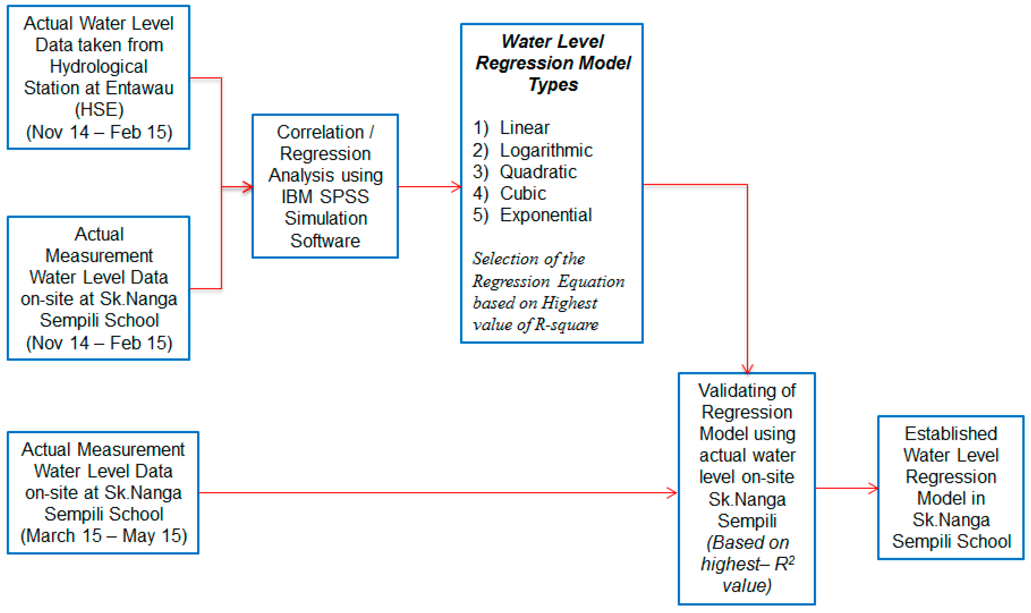
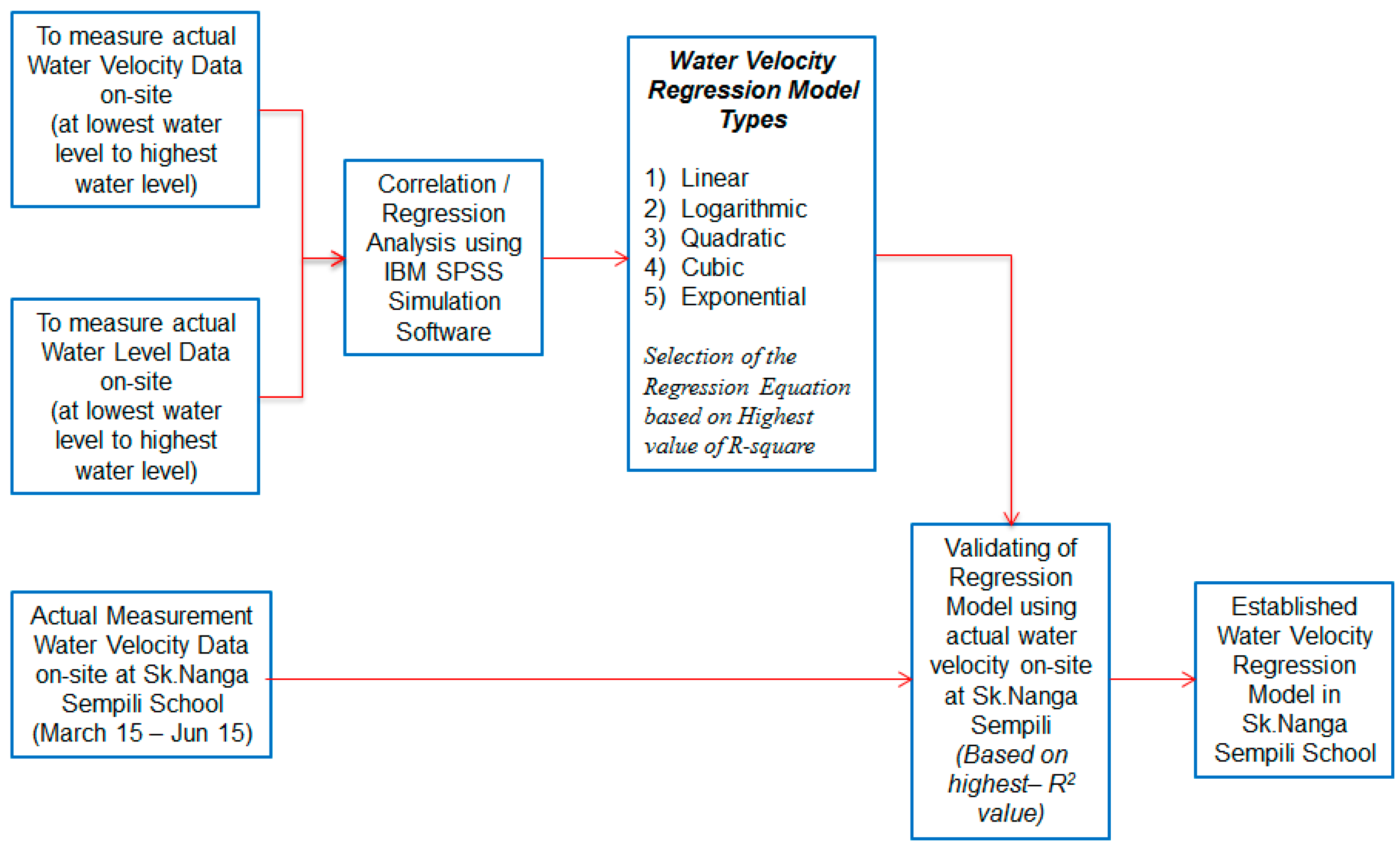
The Batang Balleh River is a branch of the Batang Rajang, especially in the area of Sk.Nanga Sempili School, which has been classified as a type-C channel river with a gradient less than 2% [21], [22]. The regression equation models for water levels and water velocity estimation at this site are suitable for this type of river only and not for the rest. The changing pattern of water velocity against water level differs based on the type of river, the slope of river and the cross-sectional profile of the river [16,22]. Due to the availability of daily average of water level and rainfall data throughout the year from the Hydrological Station at Entawau (HSE), located 20 km upstream from the project site, that data could be applied to estimate the water level and water velocity on-site at two stages of mathematical modeling regression methods by using IBM SPSS Statistics V22 software. All gathered variable data in this study must go through the correlation analysis process in order to determine the correlation between the variables before proceeding to the next process. Estimating the daily water velocity data for a year period demands two-stage regression modeling, as shown in the flowcharts displayed in Figure 2 and Figure 3.
Stage one estimates the daily average water level data on-site throughout the year by using the actual water level data accumulated from HSE. However, this stage can be omitted due to absence of a nearby hydrological station at upstream or unavailability of water level data. The regression analysis method has been used to determine the relationship of water levels at both sites by using the mathematical model equation shown in the flowchart portrayed in Figure 2.
The daily average water level data from both locations at Sk.Nanga Sempili School and HSE had been measured concurrently for 4 months (120 samples) as training data. Next, both datasets were analyzed using the regression analysis method. The regression analysis incorporates five types of regressions, such as Linear, Logarithmic, Quadratic, Cubic and Exponential curve type. The regression model equation for this study had been selected based on two criteria outlined by S. A., Bhat et al., [23], which are the highest value of coefficient of determination (R2) and the significant coefficient of correlation (p) less than 0.01, in regression simulation results represented as (Sig. < 0.01). The highest percentage of R2 coefficient (near to 1% or 100%) reflects the accuracy of modelling if it is close to the real data point. The measurement of daily water level data on-site was continued for next 3 months (90 samples) to validate the regression model equation. The regression equation modelling to be validated by using Equation (1) had proposed by John R., Tylor [24]. The regression model is considered as the best fit model if the value of the coefficient of determination (R2) value exceeds 70% [24,25,26].
R 2 = 1 i = 1 N ( y i y ^ i ) 2 i = 1 N ( y i y ¯ ) 2 ,
where N is the number of observations in the model, y is the dependent variable, y-bar is the mean of the y values and y-hat is the value predicted by the model. The numerator of the ratio is the sum of the squared differences between the actual y values and the predicted y values. The denominator of the ratio is the sum of squared differences between the actual y values and their mean.
Based on the validated regression model equation, the water level on-site was estimated throughout the year by referring to the actual daily water level data retrieved from HSE. Meanwhile, stage two estimates daily average water velocity data on-site throughout the year by using the actual water level data from the site itself. The regression analysis method was used to identify the relationship between water velocity and water level on-site, thus providing the regression model equation by adhering to the flowchart illustrated in Figure 3.
Water velocity data were measured on-site by applying the Surface Floating Method (SFM) that has been discussed in detail in Section 2.2. Water velocity of the river was measured from the lowest level (dry season) up to the highest level (flood season) with 0.5-m intervals and measurement of five times for every water level recorded. As a result, 105 samples of actual water velocity and water level data were recorded concurrently on-site as training data for regression analysis. Both datasets were analyzed by using the regression analysis method, which involved five types of regressions, such as Linear, Logarithmic, Quadratic, Cubic and Exponential curve type. The regression model equation was selected based on two criteria that had been set using the similar steps in stage one, which are highest value of coefficient of determination (R2) and the significant coefficient of correlation (p) less than 0.01 (Sig. < 0.01). The measurement of daily water velocity data on-site was continued for next 3 months (90 samples) to validate the regression model equation similar to the process in stage 1. Based on the validated regression model equation, the daily average water velocity data on-site was estimated by using the daily average water level data on-site itself. Finally, after combining both the validated regression equations of mathematical models, as discussed above, the long-term time series of the daily average water velocity data on-site had been estimated throughout the year by using the daily average water level data retrieved from HSE. These data could be employed to analyze the performance of hydrokinetic hybrid system using HOMER simulation software program.

2.1. Data Analysis Using SPSS Software

In this study, the estimation of water velocity data at the selected site was carried out by employing the regression analysis method via SPSS version 22 analysis software program [19]. Correlation analysis was performed at the initial phase for all the variables involved so as to ascertain significant correlations between the variables in deciding if a variable should be dropped or retained for further analyses. The correlation analysis refers to the method of measuring the variables or the related rank orders. In this work, all tests were analyzed by using the Pearson Correlation Analysis techniques to determine the strength of the correlations among the variables. The strength of the relationship between two variables depends on the value of coefficient of correlation (r), whereby nil relationship ranges from 0.0 to 0.3, weak ones from 0.3 to 0.5, moderate ones from 0.5 to 0.7 and strong relationship ranges from 0.7 to 1.0, thus signifying that r value closer to 1 is indicative of a perfect relationship [27,28,29,30].
In order to determine if the correlation between the variables is significant, comparison of p-value with significance level had been set. In this work, the correlation analysis employed two-tailed analysis and the test was run at p < 0.01 level of significance [23,25,29]. The correlation is significant if p < 0.01, which means a null hypothesis, is rejected and a strong relationship exists between the variables. Nonetheless, if a correlation is p > 0.01, the null hypothesis is true and the correlation is insignificant, whereby the variables are unrelated. Variables with strong correlations were retained for the next process, which was Regression Analysis, in order to obtain the best-fit model. Regression analysis refers to the statistical process that estimates the relationships between variables. The best-fit model was selected based on the highest value of coefficient of determination (R2) and the significant coefficient of correlation (p) Sig. < 0.01. The highest percentage of R2 coefficient (close to 100%) displays that the accuracy of modelling is close to the real data point.

2.2. Practical Installation Work for On-Site Data Collection

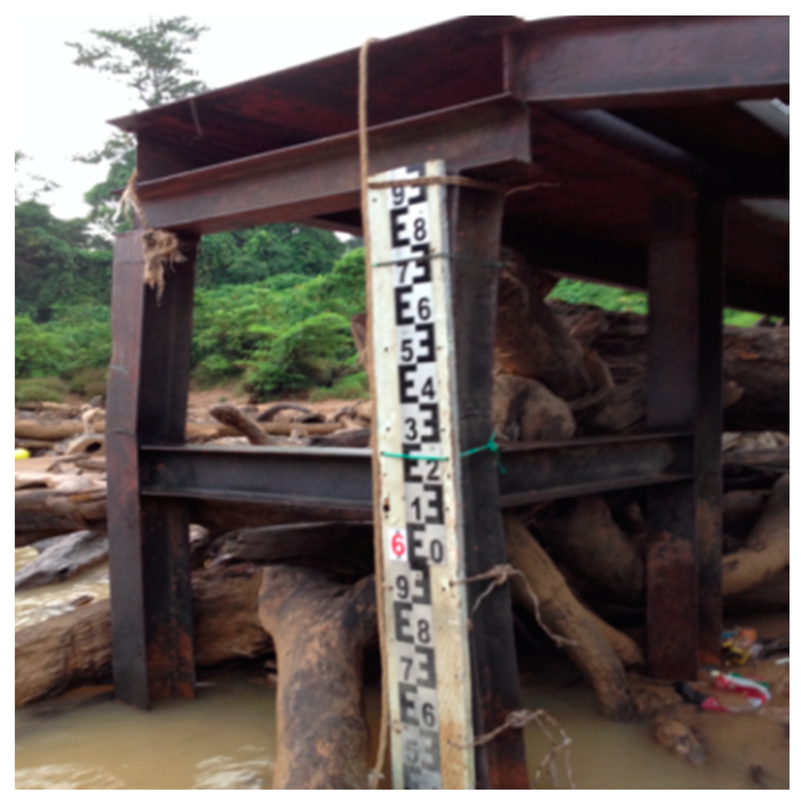
Generally, river water levels at downstream is highly affected by the amount of rainfall at the upstream. In this study, the rainfall and water level data were obtained from the HSE to determine the relationships and their impact upon water level changes on-site. Next, mathematical model equations were generated via regression analysis to estimate the water level on-site for long-term time series. As there was no hydrological station at the project site, the daily average water level data are not available. Therefore, the daily average water level data were measured on-site by installing a stick gauge, as displayed in Figure 4. The installation of a stick gauge on-site was carried out by the DID Sibu, Sarawak for water level measurement on-site. The daily water level data on-site had been measured for seven months (210 days), whereby 120 data were employed as training data, while the remaining 90 data were used for validation purpose. In addition, the water level data had been taken twice a day at 6:30 a.m. and 6:30 p.m. to adhere to the methods applied by the DID Sarawak so as to obtain daily average water level data.
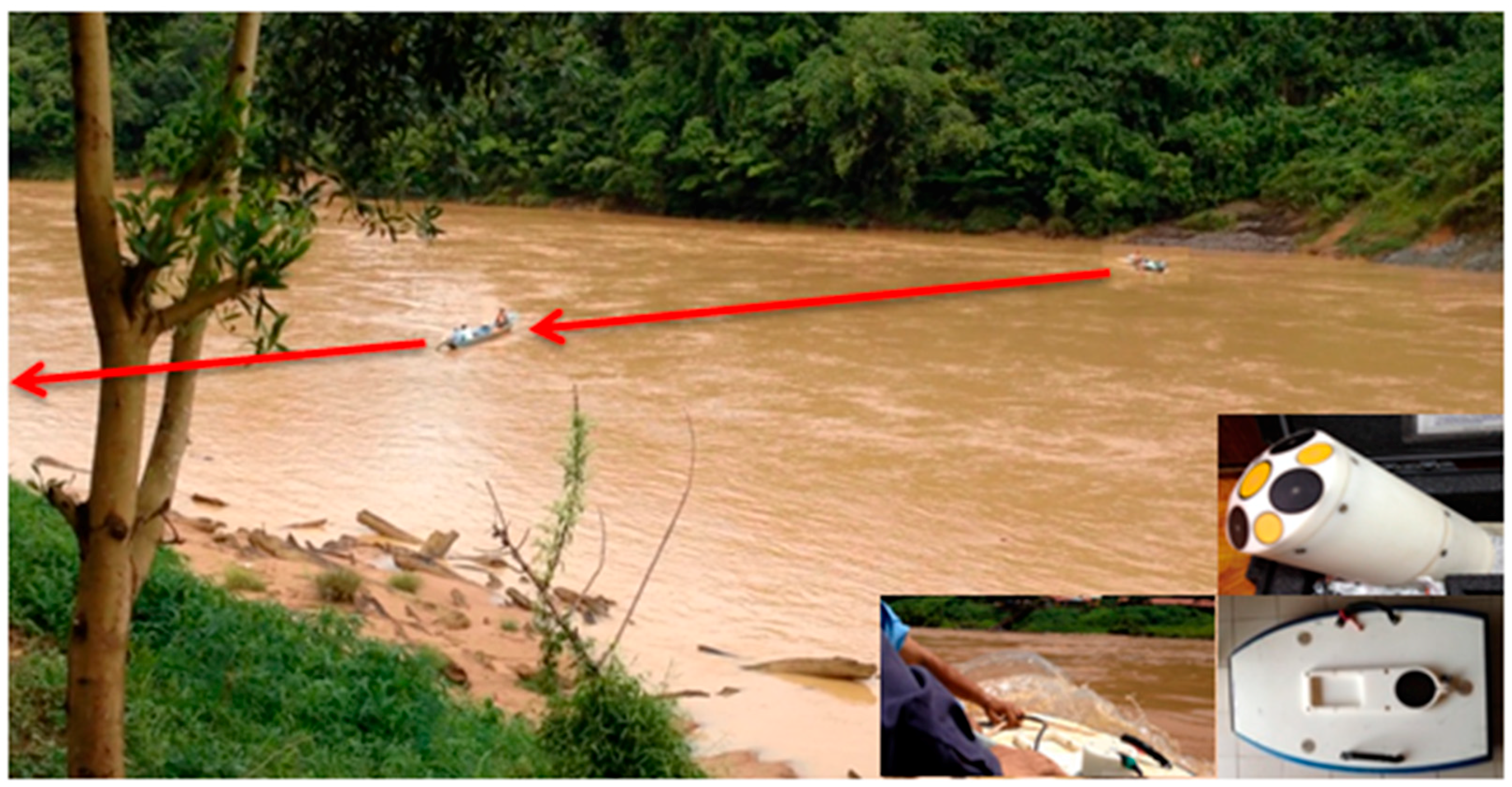
The determination of the type of river on-site had been necessary to identify the pattern of water velocity against increment of water levels. David L. Rosgen [21] divided the natural unregulated river into seven types of major streams distinguished based on channel entrenchment, channel pattern, floodplains, bedrock, cross-sectional area and slope ranges. For that purpose, the ADCP was selected as the tool to measure the profile of the Balleh River, along with its equipment commonly applied in oceanographic studies [16]. The ADCP, as operated by an expert, was mounted at the side of the boat and taken across the river in a straight line, as illustrated in Figure 5.
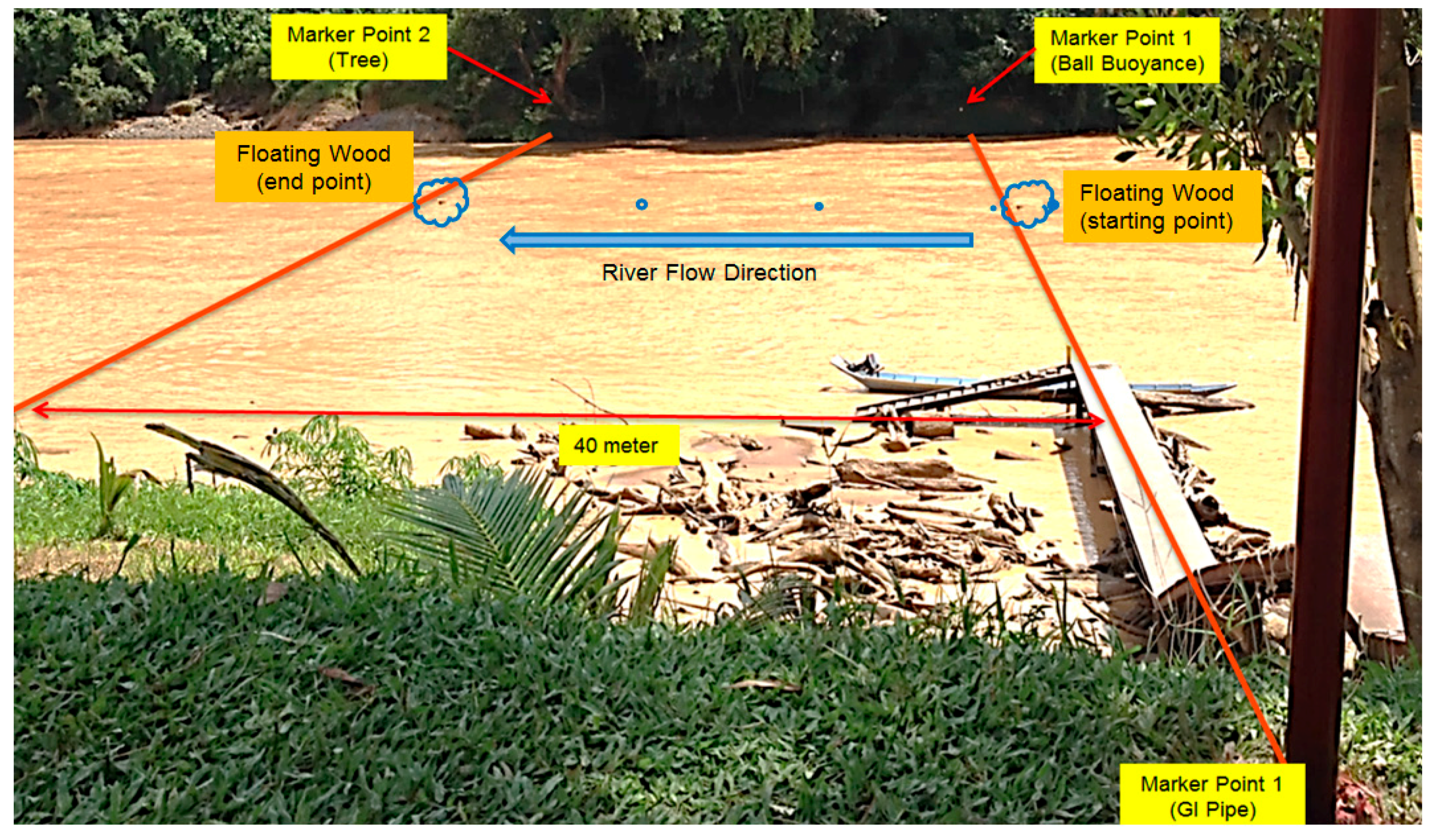
The on-site observation revealed that the Balleh River have a meandered appearance, a broad floodplain and the curve of cross-sectional area of the river is clearly shows that the Balleh River is classified into class C channel with a gradient less than 2%. The accuracy of water velocity measurement in unregulated river demands special equipment that can only be operated by experts. Hence, the most accurate method is by mounting the ADCP on rigid structures. However, as for sites without any rigid structure or bridge, the measurement should be done while in boat, which poses danger especially during floods and inaccurate outcomes of water velocity data due to the vertical and horizontal movements of the boat [30]. As for this study, the Surface Floating Method (SFM), as displayed in Figure 6, was used to measure water velocity data on-site as it is the most economical way for collecting data, which can be handled by workers without specific skill and the data could also be collected throughout the year, even during flood season [13,14,22].
The measurement of water velocity was performed by measuring the time required for a floating material to travel at a fixed distance along the stream, as illustrated in Figure 6. The floating material employed in this study was a half-submerged natural driftwood, as proposed by Cheryl C., Harrelson [22]. The procedure was repeated as many as 5 times, where the average of the values reflects the mean velocity, which was then multiplied with velocity adjustment coefficient of 0.85 in order to calculate the mean velocity of the river. This coefficient can range from 0.8 to 0.95; depending on the roughness of the channel to accommodate friction effects along the bottom and the sides of the river [14,21,22].

3. Result and Discussion

3.1. Correlation Analysis

A total 120 samples of actual water level data on-site, as well as actual water level and rainfall data obtained from HSE (as reference site), were analyzed by using the Pearson Correlation Analysis methods to determine the correlations between the variables, as depicted in Table 1. At this stage, variables that exhibited strong relationships were retained for the regression analysis process, while the rest were dropped.
Based on the results retrieved from correlation analysis, as displayed in Table 1, the water level at Entawau displayed a strong relationship with the water level on-site (Sk Nanga Sempili) with coefficient of correlation (r) = 0.939. Nonetheless, rainfall data exhibited nil correlation for both water levels at Entawau and Sk Nanga Sempili with r = −0.062 and r = 0.07, respectively. The result also showed that the significant value (p) between water level at HSE and water level on-site is p =0.000 (Sig. < 0.01), thus rejecting the null hypothesis and exhibiting significantly strong correlation between each other. This means; increment in water level at HSE caused the rising of water level on-site. A significant value (p) between rainfall data at HSE and water level at HSE is p = 0.523 (Sig. > 0.01), while the water level at Sk Nanga Sempili school is p = 0.941 (Sig. > 0.01), which means that the null hypothesis is true; the rainfall data were unrelated to the water level for both locations. Since there is a limitation in this research to obtain the entire rainfall data across the Rajang river basin, so that rainfall data only taken from HSE. It also showed that rainfall data taken at only one rain gauge station at HSE upstream failed in describing the total amount of rainfall at upstream of the river. Thus, rainfall data were omitted from the next regression analysis.

3.2. Estimation of Water Level Using Regression Analysis Method (Stage 1)

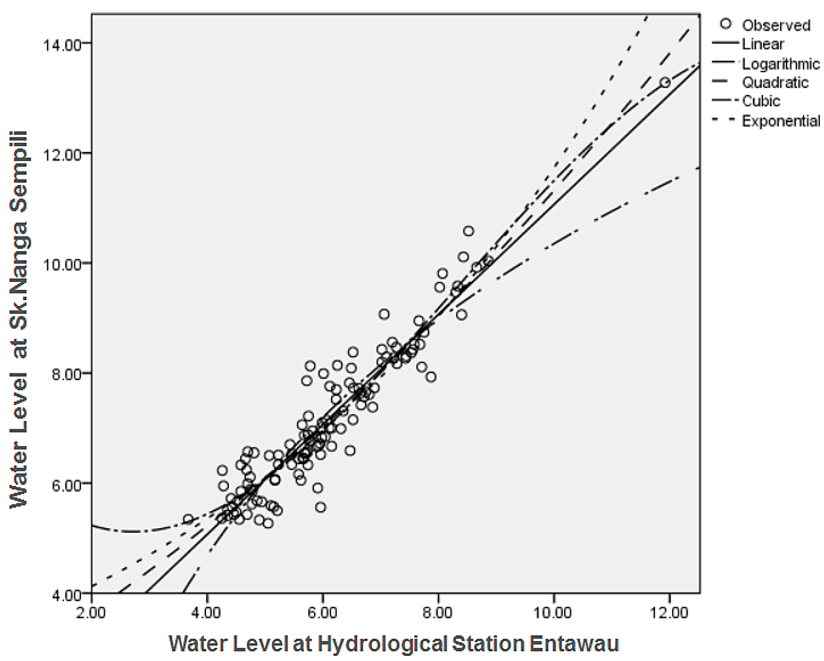
By using 120 samples of water level data at site and water level data at HSE, the regression analysis was performed by incorporating five types of regression models, as illustrated in Figure 7.
Five regression models were selected and analyzed. As a result, the regression model Cubic curve (89.1%) exemplified the highest R-square value, followed by Quadratic curve model (88.6%), Linear curve (88.2%), Exponential curve (86.3%) and logarithmic curve model (84.1%), which successfully fulfilled the first criteria. Nonetheless, the regression models of linear curve, logarithmic curve and exponential curve only satisfied the second criteria with significant coefficient of correlation (p) values below 0.01.
Out of the five types of regression models analyzed, the linear regression model was selected due to its highest value of R2 = 88.2% and all the significant coefficients of correlation (p) were 0.000 is less than 0.01 (Sig. p < 0.01) as shown in Table 2. This displayed that the water level on-site had a significantly strong correlation with the water level at HSE. From the coefficients table as shown in Table 2, the regression equation modelling is labelled as Equation (2) with a coefficient of determination at R2 = 0.882. This proves that the regression equation model is indeed accurate and required validation so as to ensure the reliability of the equation regression.
a = 0.999(b) + 1.073,
where a is the estimation water level at Sk.Nanga Sempili and b is the actual water level at hydrological station at Entawau (HSE).

Validation of Water Level Regression Modelling

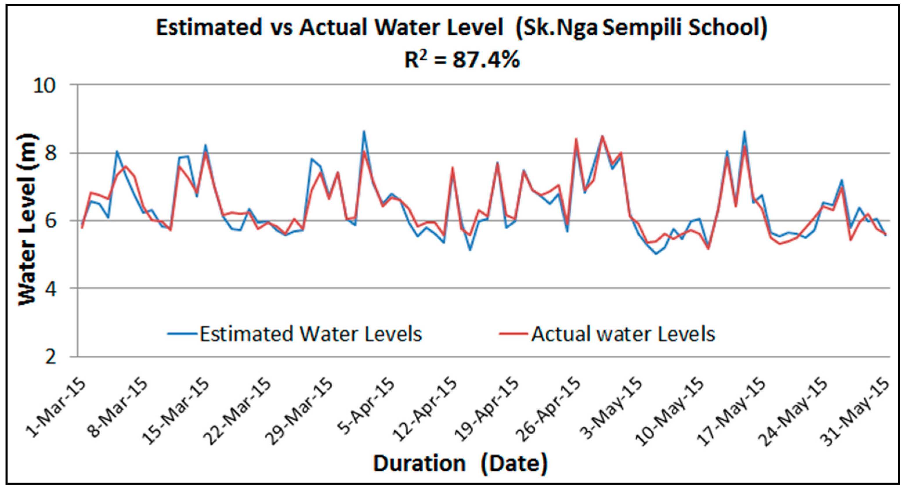
Based on the regression Equation model (2), the estimated water level on-site for 3 months recorded from March 2015 until May 2015 had been obtained. At the same period of time, the actual water level data were measured concurrently on-site for validation process, as presented in Figure 8.
The regression Equation modelling (2) was validated by using Equation (1) and the coefficient of determination (R2) result for the regression model is R2 = 87.4%, thus indicating that the regression equation modelling is accurate and could be employed to estimate long-term time series of water level on-site throughout the year.

3.3. Estimation of Water Velocity using Regression Analysis Method (Stage 2)

The measurement of water velocity at site was performed by using SFM with the correction coefficient 0.85 from the lowest level until the highest level of the river. In this work, the value 0.85 has been selected as a correction coefficient to calculate the mean velocity of the river using the Surface Floating Method (SFM), due to the water velocity value has been measured using the SFM method is very close to the water velocity value measured using ADCP logger on-site as shown in Table 3.
A total of 105 samples of the actual water level data and water velocity data at Sk Nanga Sempili had been analyzed by using the Pearson Correlation Analysis methods to determine the relationship between two variables. Based on the correlation analysis result depicted in Table 4, the water velocity and the water level at Sk Nanga Sempili displayed a strong correlation with coefficient of correlation at (r) = 0.969. The correlation analysis result, which presents the p-value of significant coefficient between water level and water velocity at Sk Nanga Sempili, is p = 0.000 (Sig. < 0.01), signifying that the null hypothesis is rejected as they exhibited significantly strong correlation between each other.
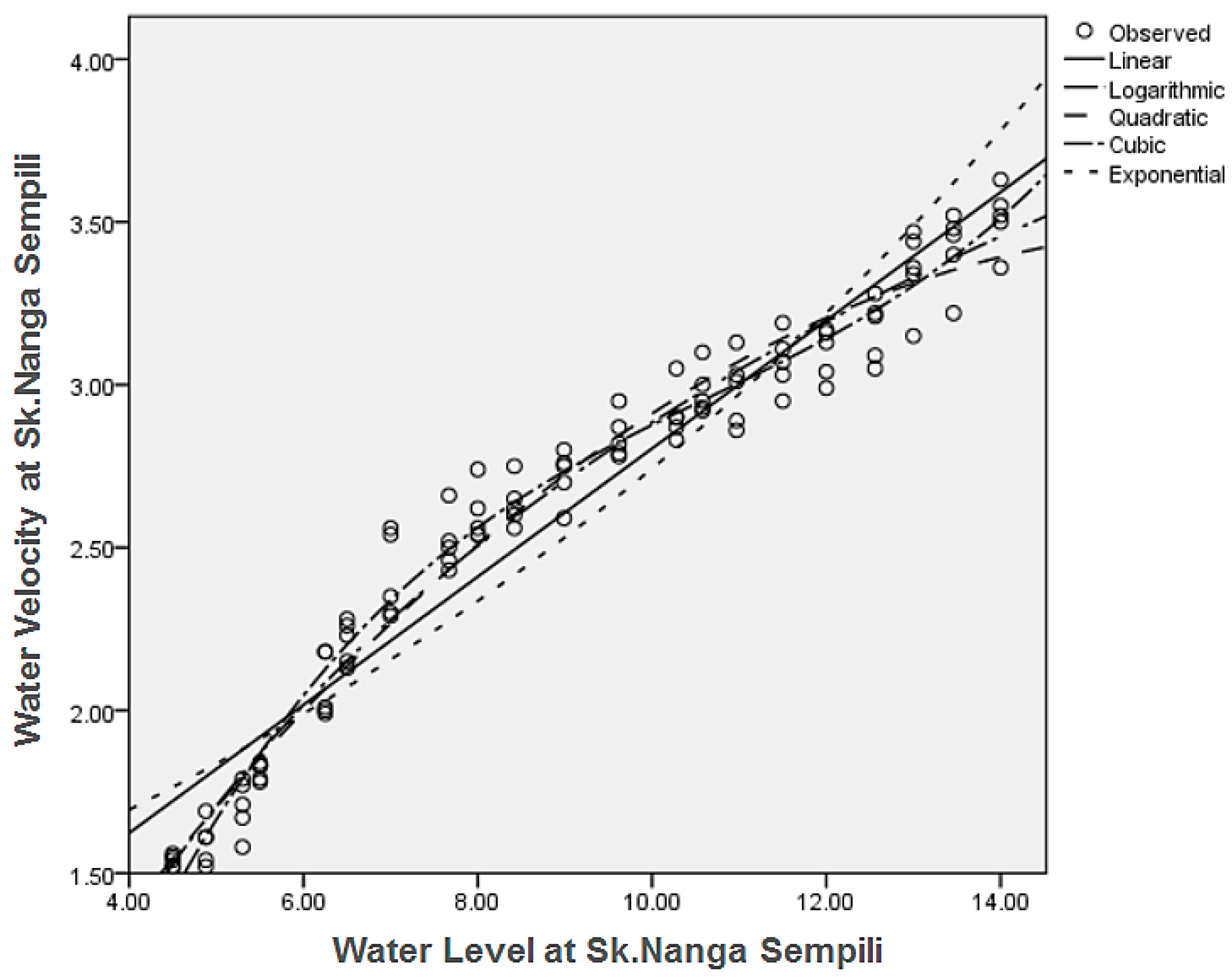
From the above result, it can be interpreted that increment in water level can significantly hike the water velocity on-site. As the parameters showed strong relationship between each other, they were retained for the next process that involved regression analysis modelling. The regression analysis was performed and involved five types of regression models, as illustrated in Figure 9 and Table 5.
Five regression models were selected and analyzed. As a result, the regression model of Cubic curve (97.7%) exhibited the highest R-square value, followed by Logarithmic curve (97.2%), Quadratic curve model (96.8%), Linear curve (94.3%) and Exponential curve model (89.6%). Nevertheless, the regression models of Cubic curve, Logarithmic curve, Linear curve and Exponential curve only satisfied the second criteria with a significant coefficient of correlation (p) less than 0.01. Out of the five types of regression models that had been selected and analyzed, the cubic regression model was selected as it fulfilled all criteria with the highest R2 = 97.7% and all significant coefficient of correlation at p < 0.01, as depicted in Table 5.
Based on the coefficients depicted in Table 5, the regression equation modelling had been derived as Equation (3) with a coefficient of determination at R2 = 97.7%. It also displayed that the regression equation modelling was accurate and required further validation to ensure the validity of the equation regression.
c = 0.003(d3) − 0.101(d2) + 1.207(d) − 2.233,
where c is the estimation water velocity at Sk.Nanga Sempili and d is the actual water level at Sk.Nanga Sempili.

Validation of Water Velocity Regression Modeling

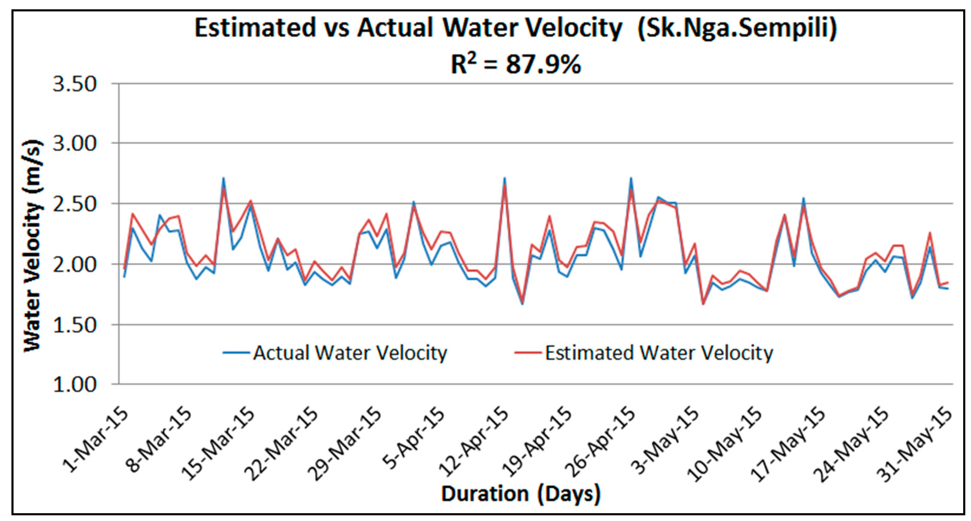
By applying the derivation of Equation (3), the estimated water velocity data on-site recorded from March 2015 until May 2015 had been generated. At the time of measurement of actual water velocity data on-site, the validation of the regression model Equation (3) had been carried out concurrently, as illustrated in Figure 10.
The regression Equation (3) was validated by using the R2 coefficient from Equation (1). The coefficient of determination result for regression modelling at R2 = 87.9% showed that the regression equation modelling is accurate and it could be used to estimate the long-term time series of water velocity on-site throughout the year. By employing the water velocity regression Equation (3), together with water level regression Equation (2), the time series of daily average water velocity data on-site had been estimated throughout the year by referring to the actual daily average water level data at the hydrological station at Entawau, as presented in Equation (4) and Table 6.
c = 0.003(a3) − 0.101(a2) + 1.207(a) − 2.233,
where c is the estimation water velocity at Sk.Nanga Sempili and a is the estimated water level at Sk.Nanga Sempili.

4. Conclusions

The Batang Balleh River, especially at Sk.Nanga Sempili School, is considered as a type-C river with a gradient less than 2%, showed that the rising water level at downstream is linearly proportional to the rise in water levels at the upstream of the river. Nevertheless, the relationship between water level and water velocity at the project site is proven to be non-linear when a polynomial/Cubic curve was applied. The standard of procedure proposed is proven to be adequate and reliable for predicting the daily average water velocity data throughout the year for unregulated rivers especially in the remote area of Kapit, Sarawak. The ability to estimate such water velocity data offers opportunities and encouragement to other researchers to continue studies pertaining to hydrokinetic power generation systems, particularly for remote area electrification in Kapit, Sarawak. Whereas the performance of the hydrokinetic system depends on the velocity of the river throughout the year. Failure to predict water velocity data accurately throughout the year will cause the hydrokinetic power generating systems to not generate electricity optimally and it will become worse if the hydrokinetic generator cannot operate. This procedure is also highly recommended to be extended to other remote area rivers around the globe, especially for project sites with limited water discharge and rainfall data. Furthermore, this method is much cheaper, safer and does not require the specific skills for data measurement on-site.

Author Contributions

Conceptualization, A.F.M.A., N.F.M. and M.A.M.R.; Methodology, A.F.M.A.; Software, A.F.M.A., N.F.M. and M.A.M.R.; Validation, A.F.M.A., N.F.M. and M.A.M.R.; Formal analysis, A.F.M.A.; Investigation, A.F.M.A.; Resources, A.F.M.A.; Data Curation, A.F.M.A., S.Z.A. and A.C.S.; Installation works on-site for data collection and measurement, A.F.M.A., K.B.M., S.Z.A. and A.C.S.; Writing-Original Draft Preparation, A.F.M.A.; Writing-Review & Editing, N.F.M. and M.A.M.R.; Visualization, N.F.M. and M.A.M.R.; Supervision, N.F.M. and M.A.M.R.; Project Administration, K.B.M.; Funding Acquisition, Ministry of Energy, Green Technology and Water, Malaysia (KeTTHA).

Funding

This research was funded by Ministry of Energy, Green Technology and Water, Malaysia (KeTTHA) and JKR Malaysia through grant number (RJ130000 .7309 4B161).

Acknowledgments

The authors would like to express their gratitude to Ministry of Energy, Green Technology and Water, Malaysia (KeTTHA) and JKR Malaysia for supporting this research of Sustainable Hydrokinetic Renewable Energy (SHRE) with the provisions of Grant (RJ130000 .7309 4B161). Most appreciated to all SHRE project team especially to Head of Project Team (SHRE), Tn.Hj. Kamarul Bahrin b Mohamad for his brilliant idea of being a pioneer in the development of Hydrokinetic Turbine Blades in Malaysia. Infinite recognition is also given to all SHRE-UPM project team members as strategic and collaborative partners who have contributed much on data retrieval work at project site and work hard to ensure the project is successful and utilized for local residents. Vast appreciation is also given to the Department of Irrigation and Drainage (DID) Sibu and Kuching, Sarawak for their contributions of installing water level stick gauge on-site, apart from providing water level and rainfall data at the Hydrological Station Entawau (HSE). A huge ‘thank you’ is also dedicated to the community of SK Nanga Sempili School for their generosity in offering a temporary site office, as well as the efforts taken to measure and to record daily data of water levels and water velocity on-site.

Conflicts of Interest

The authors declare no conflict of interest.

References

  1. Kaygusuz, K. Energy for sustainable development: A case of developing countries. Renew. Sustain. Energy Rev. 2012, 16, 1116–1126. [Google Scholar] [CrossRef]
  2. Borhanazad, H.; Mekhilef, S.; Boroumandjazi, G.; Saidur, R. Potential application of renewable energy for rural electrification in Malaysia. Renew. Energy 2013, 59, 210–219. [Google Scholar] [CrossRef]
  3. Fadaeenejad, M.; Radzi, M.A.M.; AbKadir, M.Z.A.; Hizam, H. Assessment of hybrid renewable power sources for rural electrification in Malaysia. Renew. Sustain. Energy Rev. 2014, 30, 299–305. [Google Scholar] [CrossRef]
  4. Anyi, M.; Kirke, B.; Ali, S. Remote community electrification in Sarawak, Malaysia. Renew. Energy 2010, 35, 1609–1613. [Google Scholar] [CrossRef]
  5. Vermaak, H.J.; Kusakana, K.; Koko, S.P. Status of micro-hydrokinetic river technology in rural applications: A review of literature. Renew. Sustain. Energy Rev. 2014, 29, 625–633. [Google Scholar] [CrossRef]
  6. Khan, M.J.; Bhuyan, G.; Iqbal, M.T.; Quaicoe, J.E. Hydrokinetic energy conversion systems and assessment of horizontal and vertical axis turbines for river and tidal applications: A technology status review. Appl. Energy 2009, 86, 1823–1835. [Google Scholar] [CrossRef]
  7. Güney, M.S.; Kaygusuz, K. Hydrokinetic energy conversion systems: A technology status review. Renew. Sustain. Energy Rev. 2010, 14, 2996–3004. [Google Scholar] [CrossRef]
  8. Khan, M.J.; Iqbal, M.T.; Quaicoe, J.E. Design considerations of a straight bladed darrieus rotor for river current turbines. In Proceedings of the IEEE International Symposium on Industrial Electronics, Montreal, QC, Canada, 9–13 July 2006; Volume 3, pp. 1750–1755. [Google Scholar]
  9. Behrouzi, F.; Nakisa, M.; Maimun, A.; Ahmed, Y.M. Global renewable energy and its potential in Malaysia : A review of Hydrokinetic turbine technology. Renew. Sustain. Energy Rev. 2016, 62, 1270–1281. [Google Scholar] [CrossRef]
  10. Blanco, C.; Junior, B.; de Figueiredo, N.M.; Negr, E. Assessment of hydrokinetic energy resources downstream of hydropower plants. Renew. Energy 2017, 101, 1203–1214. [Google Scholar]
  11. Lalander, E.; Grabbe, M.; Leijon, M. On the velocity distribution for hydro-kinetic energy conversion from tidal currents and rivers. J. Renew. Sustain. Energy 2013, 5, 23115:1–23115:19. [Google Scholar] [CrossRef]
  12. Previsic, M.; Bedard, R. River In-Stream Energy Conversion (RISEC) Characterization of Alaska Sites; Electric Power Research Institute: Palo Alto, CA, USA, 2008. [Google Scholar]
  13. Kusakana, K.; Vermaak, H.J. Hydrokinetic power generation for rural electricity supply: Case of South Africa. Renew. Energy 2013, 55, 467–473. [Google Scholar] [CrossRef]
  14. Kunaifi, K. Options for the Electrification of Rural Villages in the Province of Riau, Indonesia; Murdoch University: Perth, Australia, 2009. [Google Scholar]
  15. Koko, S.P.; Kusakana, K.; Vermaak, H.J. Micro-Hydrokinetic for Remote Rural Electrification. Int. J. Electr. Comput. Electron. Commun. Eng. 2014, 8, 1659–1663. [Google Scholar]
  16. Lalander, E. Hydrokinetic Resource Assessment; Uppsala University Sweden: Uppsala, Sweden, 2013. [Google Scholar]
  17. Kusakana, K.; Vermaak, H.J. Feasibility Study of Hydrokinetic Power for Energy Access in Rural South Africa. In Proceedings of the IASTED Asian Conference, Power and Energy Systems, Phuket, Thailand, 2–4 April 2012; pp. 433–438. [Google Scholar]
  18. Schulze, K.; Hunger, M.; Döll, P. Advances in Geosciences Simulating river flow velocity on global scale. Adv. Geosci. 2005, 5, 133–136. [Google Scholar] [CrossRef]
  19. IBM SPSS Statistic Version 22. 2013. Available online: https://ibm-spss-statistics-base.en.uptodown.com/windows (accessed on 2 May 2016).
  20. Ministry of Education Malaysia. Dokumen Kontrak untuk Perkhidmatan Pembekalan Elektrik Melalui Pengoperasian Dan Penyelenggaraan Set Janakuasa Bagi Sekolah-Sekolah Luar Bandar Di Negeri Sarawak Bagi Pakej 19 : Kapit 2; Contract Document (Pakej 19); Ministry of Education Malaysia: Kuala Lumpur, Malaysia, 2012. [Google Scholar]
  21. Rosgen, D.L. A Classification of Natural Rivers; Elsevier: New York, NY, USA, 1994; Volume 22, pp. 169–199. [Google Scholar]
  22. Harrelson, C.C.; Rawlins, C.L.; Potyondy, J.P. Stream Channel Reference Sites: An Illustrated Guide to Field Technique; U.S. Department of Agriculture, Forest Service, Rocky Mountain Forest and Range Experiment Station: Fort Collins, CO, USA, 1994.
  23. Bhat, S.A.; Meraj, G.; Yaseen, S.; Pandit, A.K. Statistical Assessment of Water Quality Parameters for Pollution Source Identification in Sukhnag Stream: An Inflow Stream of Lake Wular (Ramsar Site), Kashmir Himalaya. J. Ecosyst. 2014, 2014, 898054. [Google Scholar] [CrossRef]
  24. Taylor, J.R. An Introduction to Error Analysis; The Study of Uncertainties in Physical Measurements; University Sausalito California: San Rafael, CA, USA, 1997. [Google Scholar]
  25. Zhang, Z.; Tao, F.; Du, J.; Shi, P.; Yu, D.; Meng, Y.; Sun, Y. Surface water quality and its control in a river with intensive human impacts-a case study of the Xiangjiang River, China. J. Environ. Manag. 2010, 91, 2483–2490. [Google Scholar] [CrossRef] [PubMed]
  26. Liu, C.W.; Lin, K.H.; Kuo, Y.M. Application of factor analysis in the assessment of groundwater quality in a blackfoot disease area in Taiwan. Sci. Total Environ. 2003, 313, 77–89. [Google Scholar] [CrossRef]
  27. Gashi, F.; T, S.F.I.; Bilinski, H.; Shala, A.; Gashi, A. Impact of Kishnica and Badovci Flotation Tailing Dams on Levels of Heavy Metals in Water of Graçanica River (Kosovo). J. Chem. 2017, 2017. [Google Scholar] [CrossRef]
  28. Arikunto, S. Quasi Experiment; Universiti Pendidikan Indonesia: Bandung, Indonesia, 2007. [Google Scholar]
  29. Barakat, A.; El Baghdadi, M.; Rais, J.; Aghezzaf, B.; Slassi, M. Assessment of spatial and seasonal water quality variation of Oum Er Rbia River (Morocco) using multivariate statistical techniques. Int. Soil Water Conserv. Res. 2016, 4, 284–292. [Google Scholar] [CrossRef]
  30. Kuusisto, E.; Bartram, J.; Ballance, R. Chapter 12 Hydrological Measurement. In Water Quality Monitoring—A Practical Guide to the Design and Implimentation of Freshwater Quality Studies and Monitoring Programmes; Bartram, R.B.J., Ed.; United Nation Enviroment Programme: Nairobi, Kenya, 1996. [Google Scholar]
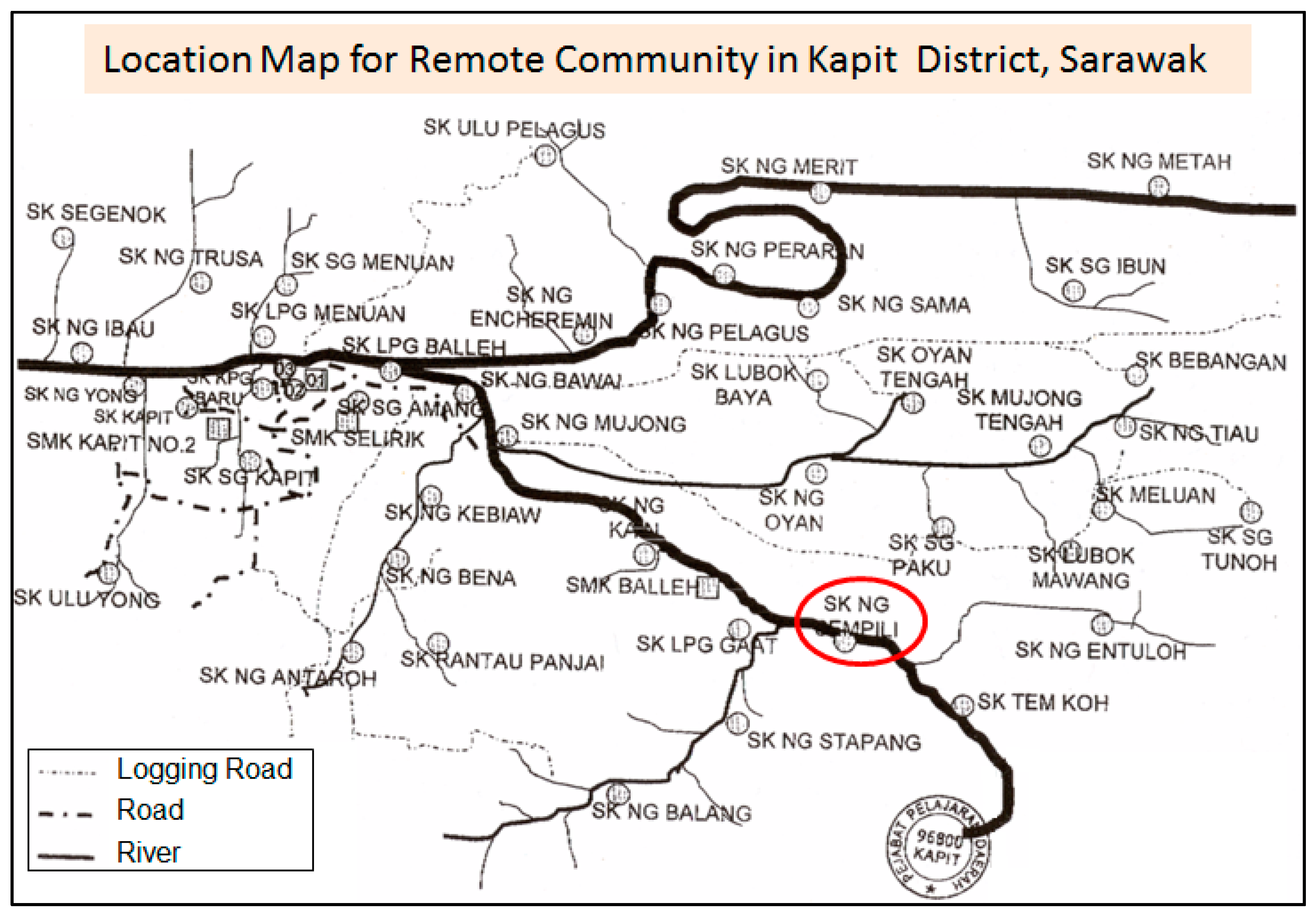
Figure 1. Pattern of population placement in rural area of Kapit, Sarawak [20].
Water 10 01330 g001
Figure 2. Flowcharts to estimate water level at Sk.Nanga Sempili School (on-site).
Water 10 01330 g002
Figure 3. Flowcharts to estimate water velocity at Sk.Nanga Sempili School (on-site).
Water 10 01330 g003
Figure 4. Stick gauge installation on-site for water level measurement.
Water 10 01330 g004
Figure 5. River profile measurement on-site using ADCP.
Water 10 01330 g005
Figure 6. Measurement of water velocity data using Surface Floating Method.
Water 10 01330 g006
Figure 7. Analysis result of five types water level regression models.
Water 10 01330 g007
Figure 8. Variance between estimated and actual water levels on-site.
Water 10 01330 g008
Figure 9. Analysis result of five types water velocity regression models.
Water 10 01330 g009
Figure 10. Variance between estimated and actual water velocity on-site.
Water 10 01330 g010
Table 1. Correlation analysis result among variables.
Rainfall Data at Entawau (HSE)Water Level Sk.Nanga Sempili
Water Level at Entawau (HSE)Pearson Correlation−0.0620.939
(Sig.) p < 0.010.5030.000
N120120
Water Level at Sk.Nanga SempiliPearson Correlation0.07-
(Sig.) p < 0.010.941-
N120-
Table 2. Regression analysis result to estimate water level on-site (Linear regression curve).
RR-SquareAdjusted R SquareStd Error of the Estimate
0.9390.8820.8810.471
Coefficients
Unstandardized Coefficients (B)Standardized Coefficients (Beta)Sig.
Water level at Entawau (HSE)0.9990.9390.000
(Constant)1.073 0.000
Note: The independent variable is Water Level at Entawau.
Table 3. Comparison of water velocity data measured using ADCP and SFM method on-site.
River Depth (m)Water Velocity Data Using:
ADCP Data Logger (m/s)Surface Floating Method (m/s)
4.881.631.59
5.831.901.88
6.252.082.07
Table 4. Correlation analysis result of water level and velocity at Sk Nanga Sempili.
Water Velocity at Sk.Nanga Sempili
Water Level at Sk.Nanga SempiliPearson Correlation (r)0.969
(Sig.) p < 0.010.000
N105
Table 5. Regression analysis result to estimate water velocity on-site (Cubic Regression Curve).
RR-SquareAdjusted R SquareStd Error of the Estimate
0.9880.9770.9760.092
Coefficients
Unstandardized CoefficientsSig.
(B)Std Error
Water level at Sk.Nanga Sempili (d)1.2070.1190.000
Water level at Sk.Nanga Sempili (d2)−0.1010.0130.000
Water level at Sk.Nanga Sempili (d3)0.0030.0000.000
(Constant)−2.2330.3280.000
Note: The independent variable is Water Level at Sk.Nanga Sempili.
Table 6. Sample form for long term of estimating water velocity data on-site.
DateActual Water Level at Hydrological Station Entawau (b)Estimated Water Level Sk.Nanga Sempili (Equation (2))Estimated Water Velocity Sk.Nanga Sempili (Equation (4))
1 March 154.82 m5.89 m1.99 m/s
2 March 155.50 m6.57 m2.19 m/s
3 March 155.44 m6.50 m2.17 m/s
4 March 155.03 m6.10 m2.05 m/s
5 March 156.99 m8.05 m2.50 m/s
6 March 156.28 m7.35 m2.37 m/s