Article

Comparison of Closed Chamber and Eddy Covariance Methods to Improve the Understanding of Methane Fluxes from Rice Paddy Fields in Japan

by
Nongpat Chaichana
1,
Sonoko Dorothea Bellingrath-Kimura
2,3,*,
Shujiro Komiya
4,†,
Yoshiharu Fujii
1,
Kosuke Noborio
5,
Ottfried Dietrich
2 and
Tiwa Pakoktom
6,*
1
United Graduate School of Agricultural Science, Tokyo University of Agriculture and Technology, Tokyo 183-8509, Japan
2
Leibniz Center of Agricultural Landscape Research (ZALF), 15374 Müncheberg, Germany
3
Institute of Agriculture and Horticulture, Faculty of Life Science, Humboldt University of Berlin, 14195 Berlin, Germany
4
Graduate School of Agriculture, Meiji University, Kanagawa 214-8571, Japan
5
School of Agriculture, Meiji University, Kanagawa 214-8571, Japan
6
Faculty of Agriculture at Kamphaeng Saen, Kasetsart University, Nakhon Pathom 73140, Thailand
*
Authors to whom correspondence should be addressed.
Current address: Department of Biogeochemical System, Max Planck Institute for Biogeochemistry, 07745 Jena, Germany.
Atmosphere 2018, 9(9), 356; https://doi.org/10.3390/atmos9090356
Submission received: 9 June 2018 / Revised: 5 September 2018 / Accepted: 13 September 2018 / Published: 15 September 2018
(This article belongs to the Special Issue C and N Cycling and Greenhouse Gases Emission in Agroecosystem)

Abstract

:
Greenhouse gas flux monitoring in ecosystems is mostly conducted by closed chamber and eddy covariance techniques. To determine the relevance of the two methods in rice paddy fields at different growing stages, closed chamber (CC) and eddy covariance (EC) methods were used to measure the methane (CH4) fluxes in a flooded rice paddy field. Intensive monitoring using the CC method was conducted at 30, 60 and 90 days after transplanting (DAT) and after harvest (AHV). An EC tower was installed at the centre of the experimental site to provide continuous measurements during the rice cropping season. The CC method resulted in CH4 flux averages that were 58%, 81%, 94% and 57% higher than those measured by the EC method at 30, 60 and 90 DAT and after harvest (AHV), respectively. A footprint analysis showed that the area covered by the EC method in this study included non-homogeneous land use types. The different strengths and weaknesses of the CC and EC methods can complement each other, and the use of both methods together leads to a better understanding of CH4 emissions from paddy fields.

1. Introduction

Rice paddy fields are important sources of the global greenhouse gas (GHG) emissions, especially methane (CH4) [1]. Atmospheric CH4 emitted from rice paddies accounts for 10 to 40% of total natural CH4 emissions. Irrigated rice areas account for 70 to 80% of the CH4 emissions from global rice production [2,3]. Methane emissions from paddy fields are a dynamic process resulting from production by methanogenic bacteria under anaerobic soils and consumption by CH4-oxidizing bacteria in aerobic conditions [4,5]. CH4 production depends on the properties of soil and management practices. For example, high rates of CH4 fluxes are found in soils with high soil organic matter content [6]. Low CH4 fluxes appear when soil contains high concentrations of ammonium and nitrate [7]. High temperatures and the increase in soil temperature stimulate the activities of soil microorganisms and, as a result, large CH4 fluxes occur [8,9]. The rice plant also plays an important role, and during rice cropping season, more than 90% of CH4 is emitted from flooded soil to the atmosphere by diffusion transport through aerenchyma cells [10].
GHG fluxes from soil have mainly been monitored by two methods: the closed chamber (CC) method and the eddy covariance (EC) method. The automatic or manually operated CC method can be used to analyse spatial variability in a field. This method is easily applied in various ecosystems and is able to capture low levels of fluxes [11]. The disadvantage of the CC method is the disturbance of the measurement point and the limitation of site and time periods, which theoretically requires more than 100 replications for a representative measurement of one site [12]. The EC method can measure continuously without disturbing the environment and can cover a few hectares, up to a large scale [13,14]. The disadvantage of the EC method is that this method requires a flat and homogeneous managed area according to canopy height and wind speed [15]. The measured values are an average of that area, which makes it difficult to identify the site-specific source and process of GHG production [16,17].
Previous studies that compared GHG fluxes as measured by the CC and EC methods showed large ranges and differences between the methods. The studies by Meijide et al. [18] and Riedere et al. [19] demonstrated that fluxes measured with the CC method were larger than those from the EC method. The possible reasons may be the non-homogeneous soil characteristics within the field and the different spatial and temporal scales. Thus, footprint analysis was suggested to assure the influence of source area [20,21]. The results from such an analysis could represent a composition of land use types within the fetch of the sensor and could be used to differentiate the contributions of fluxes from different land use types [22]. This analysis is also essential for the planning and execution of an EC tower [23].
Even though there are many studies on carbon dioxide flux measurements using CC and EC methods, few studies compare the CH4 emissions of the CC EC methods or analyse how both methods deviate and how the results can be harmonized. Thus, the objective of this study was to analyse the differences between the two methods and describe their strengths and weaknesses for use in a homogeneously managed rice paddy field at different growing stages. Furthermore, the objective of the study was to combine both methods for a more detailed description for upscaling point data to large areas and a longer time series of CH4 emission.

2. Material and Methods
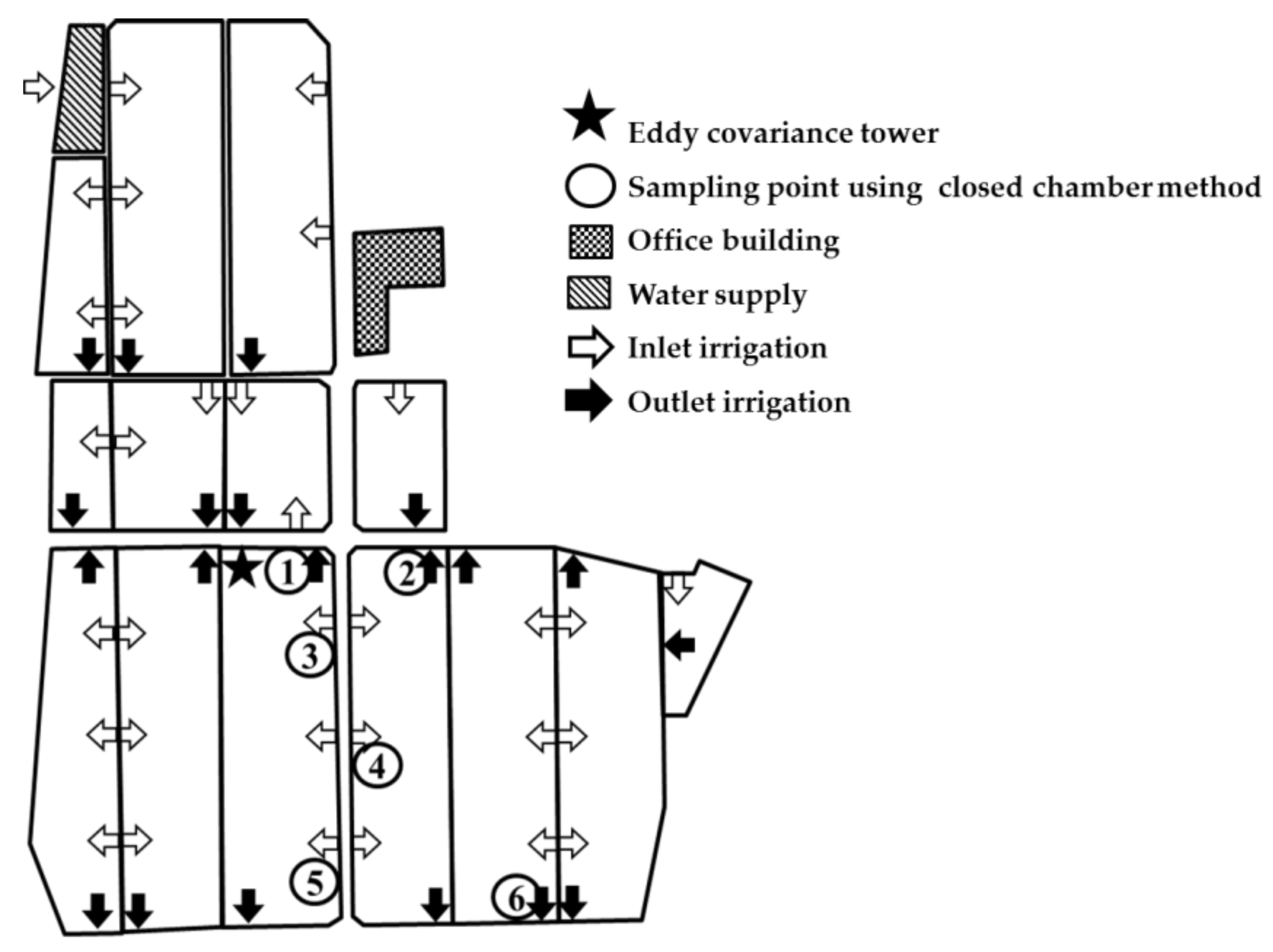
2.1. Field Design

The experimental site (35°39′56.2″ N, 139°28′17.7″ E) was located at the Field Museum Honmachi Field Science Centre, Tokyo University of Agriculture and Technology, Fuchu, Tokyo, Japan. The experiment was conducted during the paddy rice growing season from June to October 2014. The amount of annual precipitation was 1808 mm in 2014 (Japan Meteorological Agency, 2016). During the experimental period, the precipitation was 1061.5 mm and the average temperature was 24 °C, ranging from 12 to 35 °C (Figure 1). The soil is grey lowland soil (Fluvisols) [24]. At the beginning of May, basal fertilizer with 30 kg N ha−1 was applied before rice transplanting. Japonica rice variety Ikuhikari was used in most of the experimental area. Rice seedlings were transplanted on 8 May 2014. After the transplanting date, the rice paddy was flooded to 10–15 cm water depth. Mid-season drainage was conducted from 12–19 July 2014. Except for that period, the field was continuously flooded until harvest on 15 October 2014.
The EC tower was installed at the centre of the experimental site (Figure 2). Eddy covariance flux measurements were collected at a height of 1.8 m. The distance from the tower to the edge of the field in the south direction was nearly 200 m, which is large enough to cover up to approximately 100 times the tower’s height. Methane flux monitoring was conducted during the paddy rice cropping season from June to October 2014. Six sampling points of the CC method and soil gas sampling tubes were established in the field in duplicates. The wind direction of this experimental field was mainly from the south, so the sampling points were placed at the southern part of the EC measurement tower.
An intensive monitoring of CH4 fluxes and soil gas were conducted 30 days after transplant (DAT), 60 DAT, 90 DAT and after harvest (AHV). At each growing stage, 3 days of continuous sampling was conducted by the CC method, except at 30 DAT, when only 2 days were successfully sampled.
Generally, CH4 flux measurements using the CC method depend on diurnal variation of weather conditions. To reduce measurement error, researchers should avoid replacing chambers at specific times of day [19]. A previous study recommended that accurate estimation of seasonal variation of CH4 flux by the CC method at irregular time intervals depends on the growing stage of rice and that the most important period of CH4 variation is between flowering and harvest stages [25,26].

2.2. Measurement of CH4 Concentrations Using Soil Gas Sampling Tubes

The concentration of CH4 in the soil layer was sampled by soil gas sampling tubes [27]. Each soil gas sampling tube was a 30 cm long silicon tube that allowed the exchange of air, but no water, in the soil. Each tube was closed with a stopper at one end, while the other end was connected to a 30 cm long iron tube equipped with a three-way cock for gas sampling. The silicon tube was buried in the paddy field at 0, 5 or 10 cm depths in duplicates at the six CC method sampling points. A 30 mL gas sample was taken from the three-way cock location with a syringe and then transferred to a 10 mL vacuum glass vial. The CH4 concentration was analysed in the laboratory using a gas chromatograph equipped with a flame ionization detector (GC-8A, Shimadzu Corporation, Kyoto, Japan).

2.3. Measurement of CH4 Fluxes Using the Closed Chamber Method

Transparent chambers (30 cm × 30 cm × 100 cm) were used to collect the CH4 fluxes [28]. The air inside each chamber was homogenized and reduce the negative effect of air temperature by an electric fan, which was installed at the top of the chamber. To prevent leakage and soil disturbance, a chamber base was installed in the soil. Gas samples were collected using a 50 mL syringe at 0, 15 and 30 min after covering the chamber, from two chambers at each site. Daily gas sampling was carried out at 8:00, 12:00 and 16:00 for three days continuously. CH4 concentrations were analysed in the laboratory by using a gas chromatograph equipped with a flame ionization detector (GC-8A, Shimadzu Corporation, Kyoto, Japan). The detector and column were operated at 180 °C and 80 °C, respectively. The oven temperature was set at 50 °C. Helium (99.9%) was used as the carrier gas for CH4 at a flow rate of 60 mL min−1. The detection limit of CH4 gas was 0.1 ppm. Using values recorded by the CC method, methane emission rates were calculated from the increase in CH4 concentration per unit surface area of the chamber within a specific time interval. The following equation [29] was used to estimate CH4 flux values:
F = ρ × ( V A × Δ c Δ t × 273 K )
where F is CH4 flux (mg CH4 m−2 h−1), ρ is gas density of CH4 gas (0.174 mg cm−3), V is the volume of the chamber (m−3), A is the surface area of the chamber (m−2), Δct is the rate of gas concentration increase in the chamber (mg m−3 h−1) and K is Kelvin temperature of the air inside the chamber.

2.4. Measurement of CH4 Fluxes Using the Eddy Covariance Method

The eddy covariance method calculates GHG flux by measuring turbulent fluctuations in vertical wind velocities and concentration of gases [15,17]. Methane flux was determined using the following equation:
F = ρ w c ¯
where F is the turbulent flux, ρ denotes the density of the air (g m−3), w denotes the mean value of instantaneous deviation of the vertical wind velocity (m s−1) and c is the mean value of CH4 concentration (µmol mol−1).
The vertical and horizontal wind velocities and sonic temperatures (Tsv) were measured at 10 Hz intervals using a three-dimensional sonic anemometer-thermometer (SAT-540, SONIC Co., Tokyo, Japan) installed 2 m above the rice canopy. CH4/H2O fluctuation was measured at 10 Hz intervals by the closed-path EC method using a CH4/H2O closed-path gas analyser (G2301-f, Picarro Inc., Santa Clara, CA, USA). The EC raw data were processed and quality-controlled based on the TK31 software package developed by the University of Bayreuth, Germany [20]. Output computed fluxes in 30 min intervals. The footprint analysis was performed using the TK31 software package [19]. Quality assessments of the EC CH4 flux values were performed, and poor data due to the occurrence of rain events and instrument malfunction were removed. Data gaps for the CH4 fluxes were filled via linear interpolation performed on the mean diurnal variations of surrounding days [30].
In each growing stage, the land use map was overlaid with the footprint map using TK31 software. TK31 uses the foot model described by Kormann and Meixer [31] and up to two target land covers can be defined in a gridded map indicated by number. Maps were saved with suffic.asc software as ARC-GIS/ESRI-compatible ASCII grids [20]. For CH4 emissions, upscaling was performed with area-weighted averages by calculating area covers of land use maps (source areas) and multiplying by CC flux average [20,32,33].

2.5. Measurement of Soil and Environmental Parameters

At the EC tower, meteorological parameters were monitored, including net radiation (Rn: Q-7.1, Campbell Sci. Inc., North Logan, UT, USA), air temperature and relative humidity (Ta and RH: HMP60, Vaisala Inc., Helsinki, Finland), water and soil temperature at 0, 5, 10 and 20 cm soil depths (Tw and Ts: Thermo couple-T, copper and constants) and soil heat flux (G: PHF-02, PRED Inc., Tokyo, Japan). Meteorological data were sampled at 30 min intervals using data logger software (CR3000, Campbell Scientific, Inc., North Logan, UT, USA). Composite soil samples were taken from CC sampling points with two replications at each growing stage. Soil pH, electrical conductivity of soil water (mS m−1), total nitrogen (TN; g kg−1) and total carbon (TC; g kg−1) contents in soil, soil organic matter (SOM; %), ammonium ion concentration (NH4+; mg N kg−1) and nitrate ion concentration (NO3; mg N kg−1) were measured before flooding. Soil pH was measured in supernatant suspensions of a 1:2.5 soil:water mixture using a portable pHmeter equipped with a combined electrode (grass: Ag/AgCl, Horiba, Japan). Electrical conductivity of soil water was measured in supernatant suspensions of 1:5 soil:water mixture using an electrical conductivity metre (OM-51, Horiba, Japan). TN and TC were analysed using an NC analyser (Sumigraph NC-80; Sumika Chemical Analysis Service Co., Tokyo, Japan). Soil organic matter was determined from the loss in weight caused by digesting the soil with hydrogen peroxide (the hydrogen peroxide method). The concentrations of NH4+ and NO3 were determined by extracting mineral N from the soil with a 2 mol L−1 KCl solution, filtering through Whatman #42 filter paper and analysing using a colorimetric method. The absorbance of soil-extracted solutions were measured using a UV-VIS spectrophotometer (Shimadzu UV mini 1240, Shimadzu Corporation, Kyoto, Japan). Measured absorbances at 635 nm and 220 nm determined the concentrations of NH4+ and NO3, respectively. Plant growth parameters, including plant height, leaf number and tiller number, were determined from two hills at each growing stage.

2.6. Statistical Analysis of Data

The experimental data were analysed by analysis of variance (ANOVA) using R 2.13.2 (R Development Core Team; https://cran.r-project.org). A comparison among sampling points were performed using least significant differences (LSD) at p = 0.05. The stepwise regression of CH4 emissions with environmental parameters were done using the SPSS software program; Statistical Package for the Social Sciences, Version 16.0. (IBM Corp. Armonk, NY, USA).

3. Results

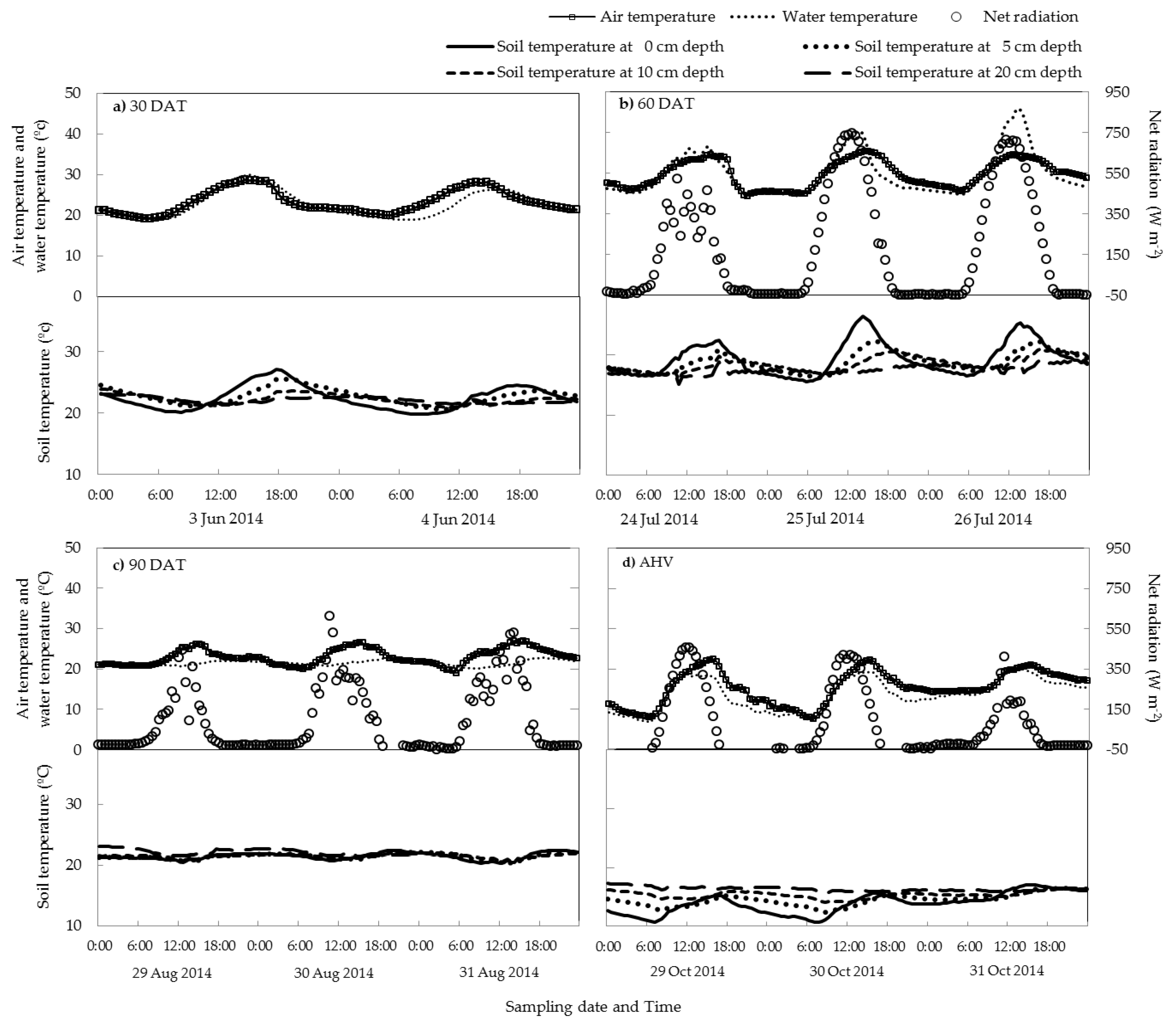
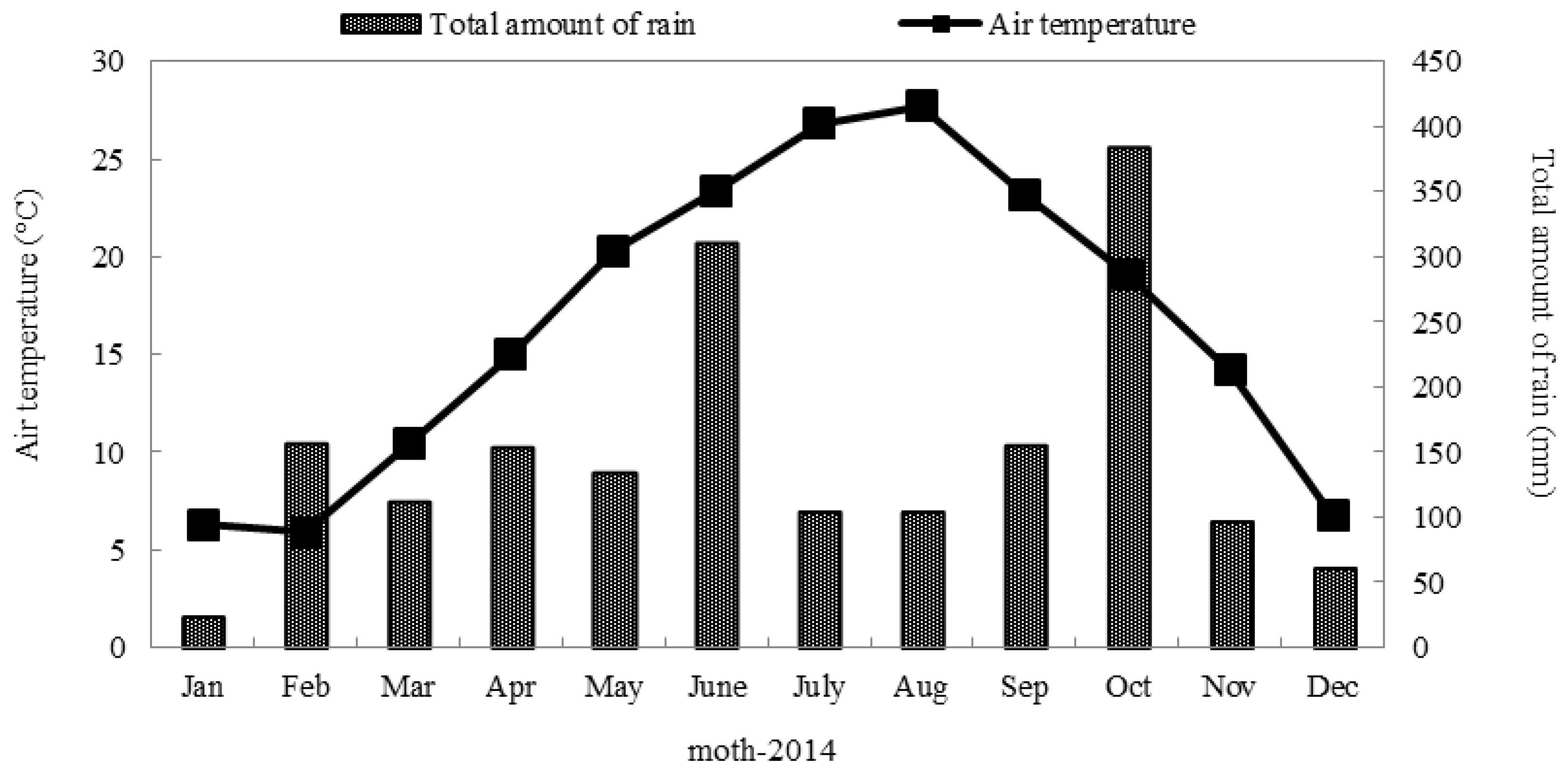
3.1. Environmental Conditions at Experimental Site

The average net radiation from June to October 2014 was 231.5 Wm−2. The daily maximum net radiation on the measurement days varied between 411.4 and 747.6 Wm−2 and was dependent on cloudiness. The radiation conditions were high at 60 DAP and low at AHV (Figure 3). Air and water temperatures showed similar patterns to the net radiation pattern. Air temperature varied from 7.5 to 35.5 °C during the experimental period. The highest value of 35.3 °C was observed at 60 DAT. During flooding conditions, the average water temperatures were 22.9, 29.9, 21.5 and 13.7 °C at 30 DAT, 60 DAT, 90 DAT and AHV, respectively. The soil temperature at 0 cm depth increased after 30 DAT and peaked at 60 DAT at 36.4 °C. At AHV, soil temperature decreased to 4 °C, according to an early winter season environment. The soil temperature difference between the 0 and 20 cm depths ranged from 0.3 to 1.9 °C during crop growth and 0 to 2.5 °C at AHV. The wind directions were from the east (60–120°), the south (180–210°), the northeast (0–45°) and the southwest (180–270°) at 30 DAT, 60 DAT, 90 DAT and AHV, respectively.
Average soil pH at the experimental site was 6.4. It was not significantly different between sampling points (Table 1). Electrical conductivities and TC were significantly different between sampling points. The values of electrical conductivity and TC at sampling point no. 3 were higher than other points.

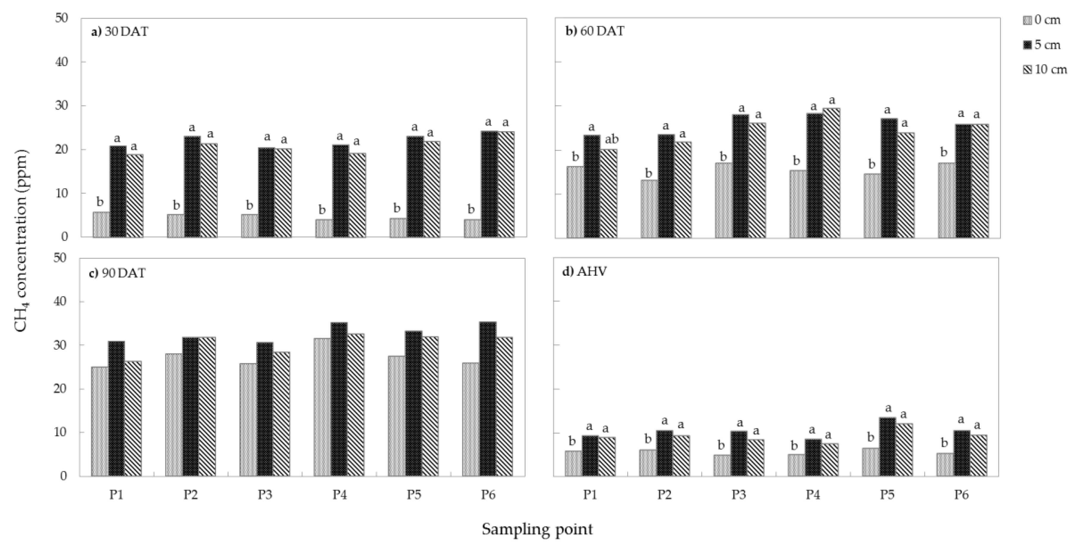
3.2. Methane Concentration in Soil

Methane concentration in paddy soil increased until 90 DAT and decreased after harvest at all soil depths (Figure 4). The concentration of CH4 in soil at 90 DAT was significantly higher than in the other periods (p < 0.01). The average concentrations at 90 DAT were 23.7, 32.8 and 30.5 ppm at 0, 5 and 10 cm soil depths, respectively. After harvest, the average CH4 concentrations decreased to 5.5, 10.3 and 9.2 ppm at 0, 5 and 10 cm soil depths, respectively. At 5 cm soil depth, the concentrations of CH4 were higher than at the 0 and 10 cm soil depths during the irrigation period. The lowest value was found at 0 cm soil depth. At 30 DAT, 60 DAT and AHV, CH4 concentrations at the 5 and 10 cm soil depths were significantly higher than those at 0 cm.

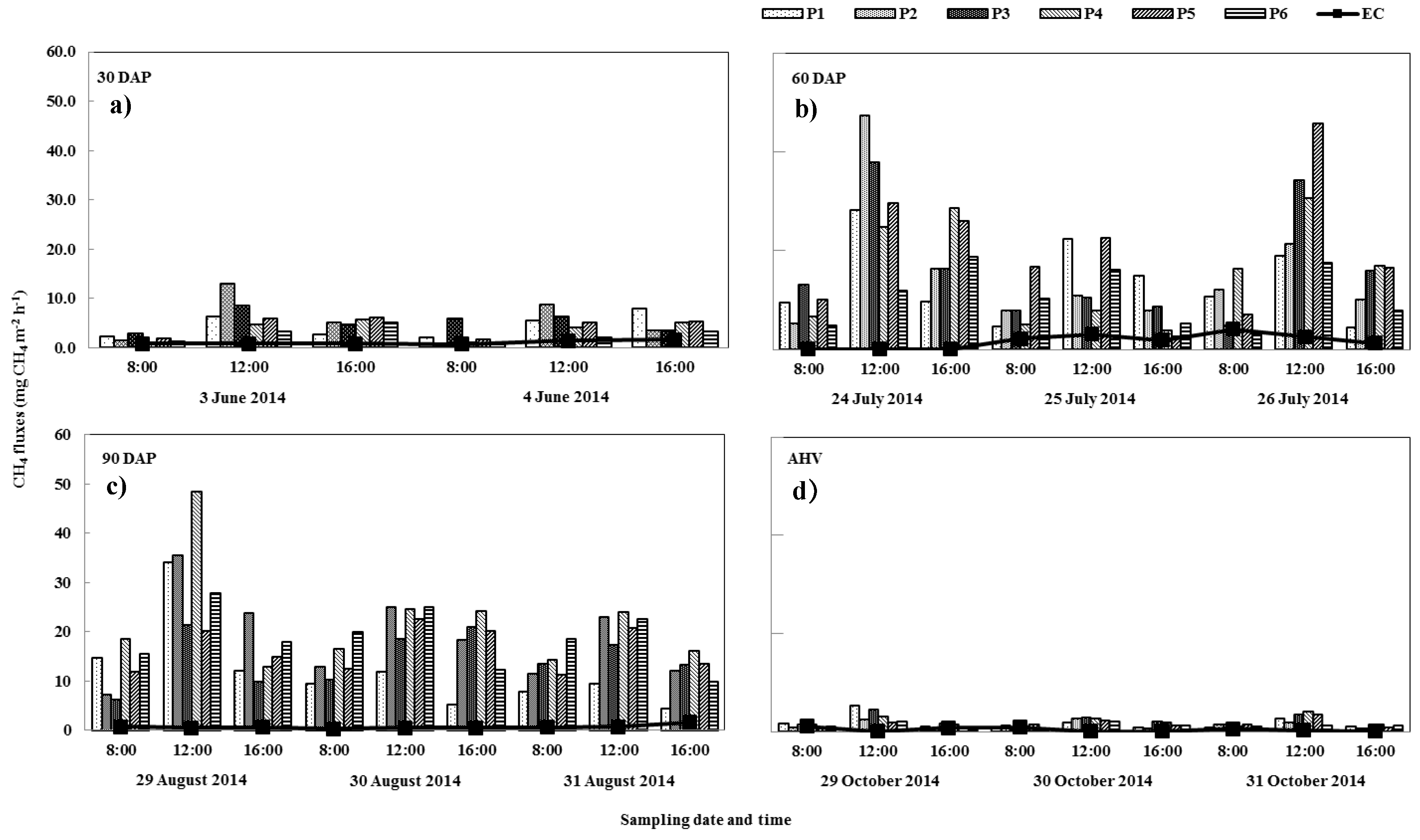
3.3. Methane Fluxes from Soil Surface

The daily pattern of CH4 flux started with low values in the early morning and increased gradually until 12:00, then it decreased again in the evening (Figure 5). Significant differences (p < 0.05) in CH4 fluxes among the 6 sampling points were found at 12:00 on 26 July 2014 (p < 0.01), 12:00 on 29 August 2014 (p < 0.01) and 12:00 on 31 August 2014. The highest CH4 flux value, 47.36 mg CH4 m−2 h−1, was found at sampling point no. 2 at 12:00 at 60 DAT, and the lowest CH4 flux value, 0.31 mg CH4 m−2 h−1, was found at sampling point no. 5 at 16:00 on 29 October 2014.
The mean CH4 flux values measured by the CC method at 30 DAT, 60 DAT, 90 DAT and AHV were 4.27, 15.27, 16.84 and 1.63 mg CH4 m−2 h−1, respectively. The CH4 fluxes measured using the CC and EC method were compared throughout the cropping season. The CC flux values were significantly greater (α = 0.05) than the EC flux values at 30 DAT, 60 DAT, 90 DAT and AHV with p-values = 0.01039, 0.00147, 0.00004 and 0.00338, respectively. The mean CH4 flux values as measured by the EC method were 1.09, 1.71, 0.66 and 0.04 mg CH4 m−2 h−1, respectively. The average CH4 fluxes calculated from the CC method were 58%, 81%, 94% and 57% higher than those of the EC method at 30 DAT, 60 DAT, 90 DAT and AHV, respectively. The CH4 flux measurements using the CC and EC methods were compared during the cropping season. CC flux was significantly greater (α = 0.05) than the EC flux at 30 DAT, 60 DAT, 90 DAT and AHV. However, the results showed the highest CH4 fluxes at 90 DAT, corresponding to the heading stage of rice production.

3.4. Influence of Environmental Factors on CH4 Flux

To evaluate the collective role of environmental factors on CH4 flux, stepwise multiple regression analysis was used for the CH4 fluxes as measured by the CC method (Table 2). The correlation equation coefficient and coefficient of determination were calculated as R = 0.67 and R2 = 0.44, respectively. The obtained f value was significant at p < 0.001 level. The environmental factors together explained 44% of the CH4 flux. The results relationship between the environment factors showed that there was a significant relationship between CH4 flux and pH, Ta_Eco, Ts_20 cm and the RH variable. Moreover, pH, EC, TC, SOM, NH4+, NO3, plant height, tiller number, Rn, Ta_Eco, Tw_Eco, Ts_10 cm, TS_CC, G, RH and WS had positive effects on the variable of increasing CH4 flux. These results showed that CH4 flux was mainly driven by Ta_Eco (β = 2.960) and Ts_10 cm (β = 2.536), followed by RH (β = 1.252).

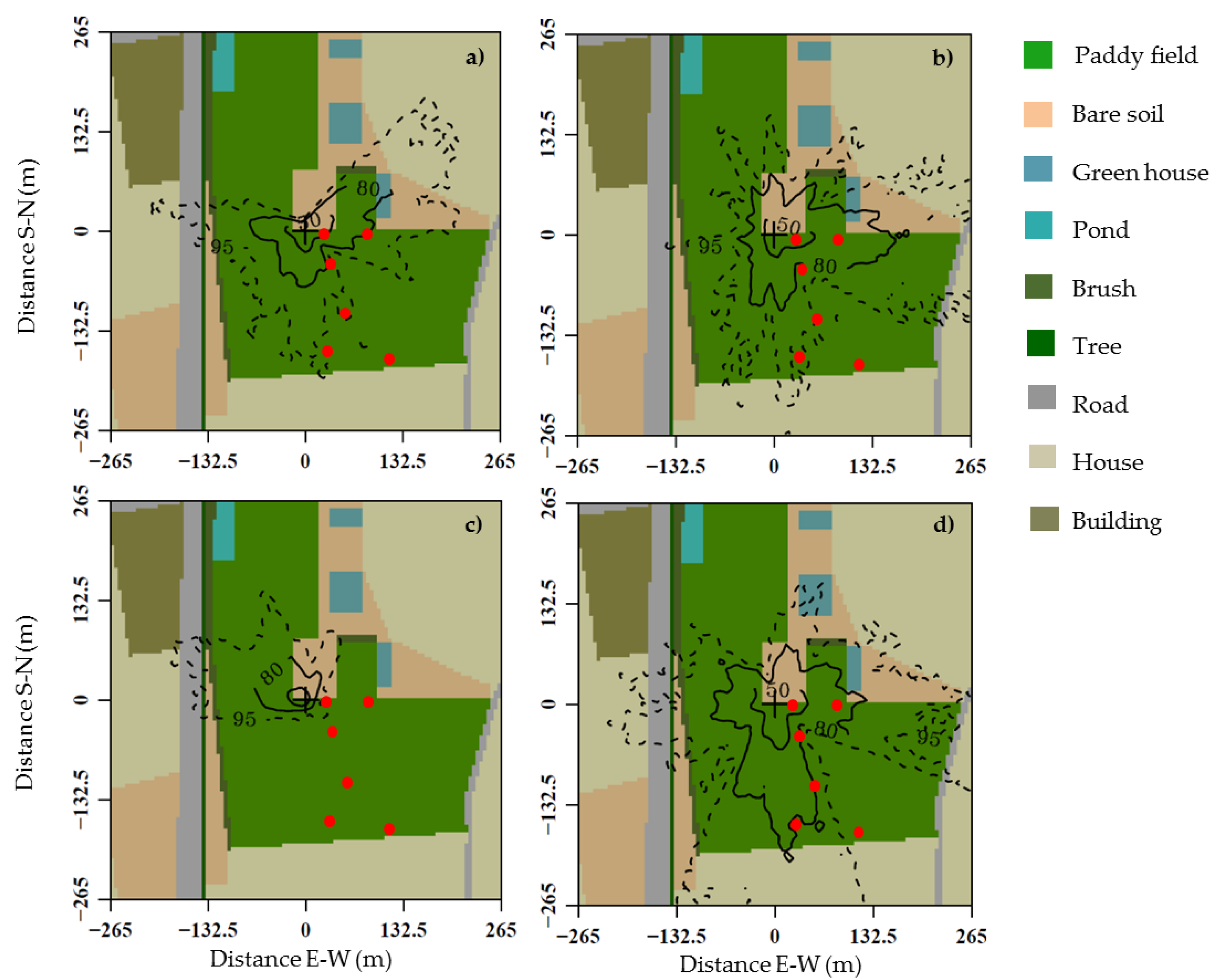
3.5. The EC Footprint Analysis and CH4 Fluxes Using CC Method

To clarify the CH4 flux source area, the flux footprint was used to analyse the source area and spatial distribution requirements of the surface source [34]. During the study, the EC footprint at 80% was representative of the scale length of the paddy rice field, bare soil and the building (Figure 6). At 30 DAT, 60 DAT, 90 DAT and AHV, EC covered 84%, 76%, 69% and 86% of the CH4 flux source areas, respectively (Table 3).

4. Discussion

4.1. Diurnal and Seasonal Variation in CH4 Emission

CH4 flux was lower in the early morning and highest at noon, then decreased again in the evening (Figure 5). Daily variations of CH4 flux showed similar emission patterns for all growing stages. The diurnal pattern of CH4 flux was similar to those of net radiation, air temperature, water temperature and soil temperature, which increased from the morning to the afternoon and decreased in the evening (Figure 3). Multiple regression analysis showed that air, water and soil temperatures had influence on CH4 concentration in soil and CH4 fluxes (Table 2). This is because increased net radiation increased the air, water and soil temperatures. Higher temperatures accelerate CH4 production by promoting methanogenic bacteria activity in soil and substrate availability. High temperatures increased CH4 sources and capacity of CH4 transport [35]. Chanton et al. [36] found that the maximum transpiration rate on midday coincided with the midday CH4 flux maximum and air and leaf temperatures and that the transpiration rate was driven by the temperature difference between leaf and atmosphere, in accordance with changing of light density [37].
CH4 flux was low in early growing stages, increased and became highest in the middle of the growing season, and then decreased after harvest (Figure 5). Flux dynamics throughout the day were also higher at 60 and 90 DAT compared to those at 30 DAT and after harvest and were much more obvious for the CC method than those for the EC method. Due to the development process of rice, high root exudate and root litter are available as substrate for methanogenic bacteria, and allow transport through the rice plant to the atmosphere [38]. The number of methanogenic bacteria increased with plant growth [39]. Previous studies indicated that the total amounts of CH4 production at the mid-season stage ripening stage ranged from 76 to 92% [40]. High root exudate and high metabolic activity due to high soil temperature favoured methane emission, and in this study, the developed rice plant induced CH4 transport more easily than did the other growing stages. Not only soil condition but also meteorological condition favoured methane emission at 60 to 90 DAT.
Molecular diffusion and ebullition of CH4 are increased as soil temperature increases [41]. The variation in solar radiation drove the differences in air-leaf temperature and humidity and are associated with convection flow in plants. Methane emissions from soil to the atmosphere are related to stomatal openings or convection flow in plants [42]. The strong radiation and high temperature conditions influenced CH4 flow through the rice plant. Additionally, tiller number was found to be positively correlated with CH4 flux (Table 2) because CH4 is released from pores connecting in the junction of the leaf sheath and the culm [35].
Although a mid-season drain during the growing season can improve aeration of the soil, it interferes with anaerobic conditions, thus leading to a decrease in CH4 emission [43]. The findings in this study indicate that after the mid-season drain, the CH4 flux was slightly higher than before the mid-season drain (Figure 5 and Table 3). This might be related to the short period of the mid-season drain and the fact that some moisture still existed in the soil, even after drain. Thus, methanogen formation resumed [44].
However, the results indicated that air temperature in the ecosystem and soil temperature at 0 cm soil depth should have had a regression correlation with CH4 flux (p value = 0.001). Both parameters were highly significant factors, with coefficient and standard coefficient effects being the most pronounced. This was similarly observed in paddy rice fields [18], and these results showed a strong correlation between soil temperature and CH4 flux during the vegetative period.

4.2. Influence of Sampling Position on CH4 Flux

Oo et al. [6] observed that average CH4 flux was lower at positions close to the irrigation channel and that high emission rates occurred at the end of the paddy rice cascade in the summer season. Different sediment deposition patterns influenced physical and chemical properties of soil depending on field position [6]. In our study, no significant trends in CH4 flux were found for inlet or outlet positions (Figure 5). This may be due to the low water flow velocity in our experimental field, since the slope differences between inlet and outlet positions within the field was very low. Thus, only EC and soil TN differed among positions and had no influence on CH4 emission rate or soil CH4 concentration (Figure 4). The variability in CH4 flux sampling points was within the range of individual chamber differences [45].

4.3. Comparison between the CC and EC Methods Used in This Study

CH4 fluxes measured by the CC method resulted from direct CH4 emissions from the soil and rice plant, and a large increase in gas concentrations had a minor influence on the atmosphere outside the chamber [46]. The chamber completely covered the ecosystem during the measurement. Weak development of stratification resulted in higher fluxes compared to those measured by the EC method [19]. Even though the use fan is recommended to diminish the overestimation of CC [47], it was not completely successful in this study. On the other hand, the EC method measured mixed fluxes from a wide area that were influenced by atmospheric turbulence [48]. The different scale and low-frequency flow pattern of turbulence may cause differences between CH4 fluxes as measured by the CC and EC methods [49]. CH4 fluxes measured by the EC method were substantially lower than those measured by the CC method, especially for measurements at high gas emission rates [50].
There were evident differences between the CH4 fluxes determined with the CC and EC methods. This may be related to the areas that influenced the measurements from the area source and the variations in CH4 emissions over the footprint area [51]. During the 90 DAT period, the southwest wind direction varied between the paddy field and bare soil. EC flux influenced the outer portion of the CC method area.
Previously, a short-term comparison of the performance of GHG flux measurements showed differences between the CH4 and CO2 emission processes at 11 and 15 days [52], and the CH4 fluxes estimated by the manual static chamber system and the EC methods agreed at six days [9].
In this study, CC fluxes were 58 to 90% higher than CH4 flux values calculated by the EC method (Figure 5). The percentage difference between the CC and EC methods in this study was larger than previous studies that showed 30% [18] or 7.6% higher values for CC compared to EC [9]. The large percentage difference between this study and previous studies can be attributed to the higher air and soil temperatures in our study site, and hence higher CH4 fluxes using the CC method. The difference in CH4 flux was larger than that reported by Yu et al. [9], who observed similar flux chamber measurements for a study conducted between 9:00 and 12:00 for 6 days. In addition, the chambers in our study were located at 3, 48, 20, 55, 90 and 123 m from the EC tower, whereas Meijide et al. [18] placed theirs in two groups, at 25 and 45 m from the EC tower. While no clear trend was found for field position, the heterogeneity of the sampling points was much higher in our study compared to theirs [18], even though our field was uniformly managed.
The results in our study came from samples collected between 8:00 and 16:00, and CH4 flux values obtained from CC and EC were compared in the same time frame. The difference between the CC and EC methods was similarly large, even if different daytime slots were compared (Table 3). The CC values were 1.5 to 24.1 times higher than the EC values during the experimental period, and 2.5 to 19.1 times higher if only the time periods between 9:00 and 14:00 were compared, as suggested in previous studies [53]. The deviation between the two methods was largest at 90 DAT. If the data from 90 DAT were deleted, the two methods showed a high correlation of R2 = 0.65 in the case of the campaign period, and R2 = 0.38 in the case of the period between 9:00 and 14:00, compared to the correlations of all periods with R2 = 0.11 and R2 = 0.22 for the campaign time and 9:00–14:00 periods, respectively. The reason the recommended 9:00-14:00 time period for CC measurements does not hold in this study may be due to the high peak captured in the CC method. Diurnal pattern of CC flux was highest at 12:00, whereas peak EC flux was observed in the late afternoon (15:00), correlating with solar radiation [9].
Comparison of the two methods showed a difference between CC and EC flux. The relative difference in diurnal pattern, according to Yu et al. [9], was due to micro-environmental changes inside the chamber inhibiting the pathway of CH4 transport to the atmosphere. Meijide et al. [18] found that differences might result from the combined effect of overestimation with CC and underestimation with EC. The higher CC flux may result from the temperature increasing when the chamber is closed [54]. Underestimation of EC flux possibly arises from mismatched observations on a non-homogeneous source or collapse of the boundary layer, followed by an extensive flux footprint under stable area stratification [55].
Reth et al. [56] reported that footprint analysis was useful to show the influence of assimilation processes on the EC tower measurements and that the differences between CC and EC methods were due to internal boundary layer effects, which occur when wind flows over different surface properties. The possible reason for the mismatch of observations between the CC and EC methods is that the CC method measure fluxes from a plot with optimal develop of plants, while the EC method combines fluxes from the field area where vegetation might not be homogeneously developed [18]. Lewicki et al. [57] reported that fluxes from the CC method cannot possibly characterise spatial-variations in source fluxes on the same time scale as the EC method. While no correlation was found for average CH4 flux between the CC and EC methods, the scaled-up CH4 flux values using the CC method, according to Sachs et al. [58], showed a strong correlation with EC flux values (R2 = 0.95; p-values = 0.02), showing that both methods are useful in showing seasonal trend. While daily fluxes are 21.1 g CH4 m−2 h−1, seasonal fluxes are 12.5 g CH4 m−2 h−1, diurnal changes in environmental conditions are driven by daily fluxes in solar radiation, air temperature and soil temperature [18].

5. Conclusions

During rice growing, the CC method showed high spatial and temporal variabilities, while the EC method illustrated the daily and seasonal changes with a high temporal resolution and a single unit for a wide area. The result from the CC method was much higher than that of the EC method and tended to overestimate due to the inclusion of optimally grown rice plants at high temperatures for flux measurements, and the EC method aggregated different sources and masked the individual processes behind the fluxes at each point. The daily variations in CH4 fluxes from both methods showed similar emission patterns for all growing stages and showed significant correlation, as both methods scaled up to the same spatial scale. To capture the heterogeneity within the field, the CC method is predicated on its mobile facility and direct link to measurement point. With the analysis of continuous measurements that show the general trend of a larger area, the EC method has a strong advantage. The different strengths and weaknesses of the CC and EC methods can complement each other, and the use of both methods together leads to more understanding of CH4 emissions from paddy fields.

Author Contributions

All authors contributed to the research and to the collaboration of this manuscript; N.C. perform the data collection, analysis and prepare the first draft of this paper; S.K and K.N. performed the field experimental and eddy covariance work; Y.F. and T.P. supervised the overall research work; O.D. processed the data analysis; S.D.B.-K. provided guidelines for the write up of the manuscript and contributed to its editing and finalization.

Funding

This research was partly supported by Grant-in-Aid for Scientific Research (A) (25252044).

Acknowledgments

The first author sincerely thanks the Japanese government (Monbukakusho: MEXT) scholarship association for supporting this research. We thank Wolfgang Babel from the Institute of Micrometeorology of University of Bayreuth for providing the footprint analysis tool and assisting us with the application of the tool. The publication of this article was funded by the Open Access Fund of the Leibniz Association.

Conflicts of Interest

The authors declare no conflict of interest.

References

  1. Wassmann, R.; Papen, H.; Rennenberg, H. Methane Emission from rice paddies and possible mitigation strategies. Chemosphere 1993, 26, 201–217. [Google Scholar] [CrossRef]
  2. Wassmann, R.; Neue, H.U.; Lantin, R.S.; Makarim, K.; Chareonsilp, N.; Buendia, L.V.; Rennenberg, H. Characterization of methane emissions from rice fields in Asia II. Differences among irrigated, rainfed, and deepwater rice. Nutr. Cycl. Agroecosyst. 2000, 58, 13–22. [Google Scholar] [CrossRef]
  3. Zschornack, T.; Bayer, C.; Zanatta, J.; Vieira, F.; Anghinoni, I. Mitigation of methane and nitrous oxide emissions from flood-irrigated rice by no incorporation of winter crop residues into the soil. Rev. Bras. Cienc. Solo 2011, 35, 623–634. [Google Scholar] [CrossRef] [Green Version]
  4. Whalen, S.C. Biogeochemistry of methane exchange between natural wetlands and the atmosphere. Environ. Eng. Sci. 2005, 22, 73–94. [Google Scholar] [CrossRef]
  5. Hendriks, D.M.D.; van Huissteden, J.; Dolman, A.J. Multi-technique assessment of spatial and temporal variabitity of methane fluxes in a peat meadow. Agric. For. Meteorol. 2010, 150, 757–774. [Google Scholar] [CrossRef]
  6. Oo, A.Z.; Nguyen, L.; Win, K.T.; Cadisch, G.; Bellingrath-Kimura, S.D. Toposequential variation in methane emissions from double-cropping paddy rice in Northwest Vietnam. Geoderma 2013, 209–210, 41–49. [Google Scholar] [CrossRef]
  7. Castro, M.S.; Steudler, P.A.; Melillo, J.M.; Aber, J.D.; Bowden, R.D. Factor controlling atmospheric methane consumption by temperate forest soils. Glob. Biogeochem. Cycles 1995, 9, 1–10. [Google Scholar] [CrossRef]
  8. Komiya, S.; Noborio, K.; Shoji, Y.; Yazaki, T.; Theerayut, T. Measuring CH4 flux in a rice paddy field in Thailand using relaxed eddy accumulation (REA) method. J. Jpn. Soc. Soil Phys. 2014, 128, 23–31. (In Japanese) [Google Scholar]
  9. Yu, L.; Wang, H.; Wang, G.; Song, W.; Huang, Y.; Li, S.-G.; Liang, N.; Tang, Y.; He, J.-S. A comparison of methane emission measurements using eddy covariance and manual and automated chamber-based techniques in Tibetan Plateau alpine wetland. Environ. Pollut. 2013, 181, 81–90. [Google Scholar] [CrossRef] [PubMed]
  10. Jia, Z.; Cai, Z.; Xu, H.; Li, X. Effect of rice plants on CH4 production, transport, oxidation and emission in rice paddy soil. Plant Soil 2001, 230, 211–221. [Google Scholar] [CrossRef]
  11. Kimura, M.; Miura, Y.; Watanabe, A.; Katoh, T.; Haraguchi, H. Methane Emission from Paddy Field (Part 1) Effect of Fertilization, Growth Stage and Midsummer Drainage: Pot Experiment. Environ. Sci. 1991, 4, 265–271. [Google Scholar] [CrossRef]
  12. Katayanagi, N.; Hatano, R. Spatial variability of greenhouse gas fluxes from soils of various land uses on a livestack farm in Southern Hokkaida, Japan. Phyton 2005, 45, 309–318. [Google Scholar]
  13. Pakoktom, T.; Chaichana, N.; Phattaralerphong, J.; Sathornkich, J. Carbon Use Efficiency of the First Ratoon Cane by Eddy Covariance Technique. Int. J. Environ. Sci. Dev. 2013, 4, 488–491. [Google Scholar] [CrossRef]
  14. Komiya, S.; Noborio, K.; Katano, K.; Kondo, F. Methane and carbon dioxide dynamics over a rice-cropping season in Japan. In Proceedings of the AsiaFlux Workshop 2014 “Bridging Atmospheric Flux Monitoring to National and International Climate Change Initiatives”, Los Banos, Philippines, 18–23 August 2014; AsiaFlux: Los Banos, Philippines, 2014. [Google Scholar]
  15. Baldocchi, D. Assessing the eddy covariance technique technique for evaluating carbon dioxide exchange rates of ecosystems: Past, present and future. Glob. Chang. Biol. 2003, 9, 479–492. [Google Scholar] [CrossRef]
  16. Liu, H.Z.; Feng, J.W.; Järvi, L.; Vesala, T. Four-year (2006–2009) eddy covariance measurements of CO2 flux over an urban area in Beijing. Atmos. Chem. Phys. 2012, 12, 7881–7892. [Google Scholar] [CrossRef]
  17. Wang, K.; Zheng, X.; Pihlatie, M.; Vesala, T.; Liu, C.; Haapanala, S.; Mammarella, I.; Rannik, Ü.; Liu, H. Comparison between static chamber and tunable diode laser-based eddy covariance techniques for measuring nitrous oxide fluxes from a cotton field. Agric. For. Meteorol. 2013, 171–172, 9–19. [Google Scholar] [CrossRef]
  18. Meijide, A.; Manca, G.; Goded, I.; Magliulo, V.; di Tommasi, P.; Seufert, G.; Cescatti, A. Seasonal trends and environmental controls of methane emissions in a rice paddy field in Northern Italy. Biogeosciences 2011, 8, 3809–3821. [Google Scholar] [CrossRef] [Green Version]
  19. Riederer, M.; Serafimovich, A.; Foken, T. Net ecosystem CO2 exchange measurements by the closed chamber method and the eddy covariance technique and their dependence on atmospheric conditions. Atmos. Meas. Tech. 2014, 7, 1057–1064. [Google Scholar] [CrossRef] [Green Version]
  20. Mauder, M.; Foken, T. Documentation and Instruction Manual of the Eddy-Covariance Software Package TK3 (Update). Available online: https://epub.uni-bayreuth.de/id/eprint/2130 (accessed on 10 February 2015).
  21. Schmid, H.P. Footprint modeling for vegetation atmosphere exchange studies; a review and perspective. Agric. For. Meteorol. 2002, 113, 159–183. [Google Scholar] [CrossRef]
  22. Aubinet, M.; Vesala, T.; Papale, D. Eddy Covariance: A Practical Guide to Measurement and Data Analysis; Springer: Dordrecht, UK, 2012; p. 438. [Google Scholar]
  23. Burba, G. Illustration of flux footprint estimates affected by measurement height, surface roughness and thermal stability. In Automated Weather Stations for Applications in Agriculture and Water Resources Management; Hubbards, K., Sivakumar, M., Eds.; World Meteorological Organization: Geneva, Switzerland, 2001; pp. 77–86. [Google Scholar]
  24. Food and Agriculture Organization of the United Nations. FAO-Unesco Soil Map of the World: Legend; UNESCO: Paris, France, 1971. [Google Scholar]
  25. Buendia, L.V.; Neue, H.U.; Wassmann, R.; Lantin, R.S.; Javellana, A.M.; Arah, J.; Wang, Z.; Wangfang, L.; Makarim, A.K.; Corton, T.M.; et al. An efficient sampling strategy for estimating methane emission from rice field. Chemosphere 1998, 36, 395–407. [Google Scholar] [CrossRef]
  26. Minami, K.; Yagi, K.; Tokida, T.; Sander, B.O.; Wassmann, R. Appropriate frequency and time of day to measure methane emissions from an irrigated rice paddy in Japan using the manual closed chamber method. Greenh. Gas Meas. Manag. 2012, 2, 118–128. [Google Scholar] [CrossRef]
  27. Kusa, K.; Sawamoto, T.; Hu, R.; Hatano, R. Comparison of N2O and CO2 concentrations and fluxes in the soil profile between a Gray Lowland soil and an Andosol. J. Soil Sci. Plant Nutr. 2010, 56, 186–199. [Google Scholar] [CrossRef]
  28. Theint, E.E.; Suzuki, S.; Ono, E.; Bellingrath-Kimura, S.D. Influence of different rates of gypsum application on methane emission from saline soil related with rice growth and rhizosphere exudation. Catena 2015, 133, 467–473. [Google Scholar] [CrossRef]
  29. Mu, Z.; Kimura, S.D.; Hatano, R. Estimation of global warming potential from upland cropping systems in central Hokkaido, Japan. J. Soil Sci. Plant Nutr. 2006, 52, 371–377. [Google Scholar] [CrossRef] [Green Version]
  30. Qun, D.; Huizhi, L. Seven years of carbon dioxide exchange over a degraded grassland and cropland wiht ecosystems in a semiarid area of China. Agric. Ecosyst. Environ. 2013, 173, 1–12. [Google Scholar] [CrossRef]
  31. Kormann, R.; Meixner, F.X. An analytical footprint model for non-neutral stratification. Bound.-Layer Meteorol. 2000, 99, 207–224. [Google Scholar] [CrossRef]
  32. Becker, T.; Kutzbach, L.; Forbrich, I.; Schneider, J.; Jager, D.; Thees, B.; Wilmking, M. Do we miss the hot spots?—The use of very high resolution aerial photographs to quantify carbon fluxes in peatlands. Biogeosciences 2008, 5, 1387–1393. [Google Scholar] [CrossRef]
  33. Budishchev, A.; Mi, Y.; van Huissteden, J.; Belelli-Marchesini, L.; Schaepman-Strub, G.; Parmentier, F.J.W.; Fratini, G.; Gallagher, A.; Maximov, T.C.; Dolman, A.J. Evaluation of a plot-scale methane emission model using eddy covariance observation and footprint modelling. Biogeosciences 2014, 11, 4651–4664. [Google Scholar] [CrossRef] [Green Version]
  34. Baldocchi, D. Flux footprints within and over forest canopies. Bound.-Layer Meteorol. 1997, 85, 273–292. [Google Scholar] [CrossRef]
  35. Neue, H.U.; Wassmann, R.; Kludze, H.K.; Bujun, W.; Lantin, R.S. Factors and processes controlling methane emissions from rice fields. Nutr. Cycl. Agroecosyst. 1997, 49, 111–117. [Google Scholar] [CrossRef]
  36. Chanton, J.P.; Whiting, G.J.; Blair, N.E.; Lindau, C.W.; Bollich, P.K. Methane emission from rice: Stable isotopes, diurnal variations, and CO2 exchange. Glob. Biogeochem. Cycles 1997, 11, 15–27. [Google Scholar] [CrossRef]
  37. Dacey, J.W.H. Internal winds in water lilies: An adaptation for life in anaerobic sediments. Science 1980, 210, 1017–1019. [Google Scholar] [CrossRef] [PubMed]
  38. Nouchi, I.; Hosono, T.; Aoki, K.; Minami, K. Seasonal variation in methane flux from rice paddies associated with methane concentration in soil water, rice biomass and temperature, and its modelling. Plant Soil 1994, 161, 195–208. [Google Scholar] [CrossRef]
  39. Bosse, U.; Frenzel, P. Activity and distribution of methane-oxidizing bacteria in flooded rice soil microcosms and in rice plants (Osyza sativa). Appl. Environ. Microbiol. 1997, 63, 1199–1207. [Google Scholar] [PubMed]
  40. Yang, S.-S.; Chang, H.-L. Diurnal variation of methane emission from paddy fields at different growth stages of rice cultivation in Taiwan. Agric. Ecosyst. Environ. 1999, 76, 75–84. [Google Scholar] [CrossRef]
  41. Alberto, M.C.R.; Wassmann, R.; Buresh, R.J.; Quilty, J.R.; Correa, T.Q., Jr.; Sandro, J.M.; Centeno, C.A.R. Measuring methane flux from irrigated rice fields by eddy covariance method using open-path gas analyzer. Field Crops Res. 2014, 160, 12–21. [Google Scholar] [CrossRef]
  42. Wang, Z.-P.; Han, X.-G. Diurnal variation in methane emissions in relation to plants and environmental variables in the Inner Mongolia marshes. Atmos. Environ. 2005, 39, 6295–6305. [Google Scholar] [CrossRef]
  43. Zhang, Y.; Sachs, T.; Li, C.; Boike, J. Upscaling methane fluxes from closed chambers to eddy covariance based on a permaforest biogeochemistry integrated model. Glob. Chang. Biol. 2012, 18, 1428–1440. [Google Scholar] [CrossRef]
  44. Tariq, A.; Vu, Q.D.; Jensen, L.S.; de Tourdonnet, S.; Sander, B.O.; Wassmann, R.; Mai, T.V.; de Neergaard, A. Mitigating CH4 and N2O emissions from intensive rice production systems in northern Vietnam: Efficiency of drainage pattern in combination with rice residue incorpation. Agric. Ecosyst. Environ. 2017, 249, 101–111. [Google Scholar] [CrossRef]
  45. Clements, R.J.; Verma, S.B.; Verry, E.S. Relating chamber measurements to eddy correlation measurements of methane flux. J. Geophys. Res. 1995, 100, 21047–21056. [Google Scholar] [CrossRef]
  46. Schrier-Uijl, A.P.; Kroon, P.S.; Hensen, A.; Leffelaar, P.A.; Berendse, F.; Veenendaal, E.M. Comparison of chamber and eddy covariance-based CO2 and CH4 emission estimates in a heterogeneous grass ecosystem on peat. Agric. For. Meteorol. 2010, 150, 825–831. [Google Scholar] [CrossRef]
  47. Brændholt, A.; Larsen, K.S.; Ibrom, A.; Pilegaard, K. Overestimation of closed-chamber soil CO2 effluxes at low atmospheric turbulence. Biogeosciences 2017, 14, 1603–1616. [Google Scholar] [CrossRef]
  48. Foken, T.; Aubinet, M.; Leuning, R. The eddy-covariance method. In Eddy Covariance: A Pratical Guide to Measurements and Data Analysis; Aubinet, M., Vesala, T., Papale, D., Eds.; Springer: Heidelberg, Germany, 2012; pp. 1–9. [Google Scholar]
  49. Thomas, C.; Foken, T. Flux contribution of coherent structures and its implications for the exchange of energy and matter in a tall spruce canopy. Bound.-Layer Meteorol. 2007, 123, 317–337. [Google Scholar] [CrossRef]
  50. Bolstad, P.V.; Davis, K.J.; Martin, J.; Cook, B.D.; Wang, W. Component and whole-system respiration fluxes in northern deciduous forest. Tree Physiol. 2004, 24. [Google Scholar] [CrossRef]
  51. Christensen, S.; Ambus, P.; Arah, J.R.M.; Claton, H.; Galle, B.; Griffith, W.T.; Hargreaves, K.J.; Klemedtsson, L.; Lind, A.M.; Maag, M.; et al. Notrous oxide emission from an agricultural field: Comparison between measurements by flux chamber and micrometerological techniques. Atmos. Environ. 1996, 30, 4183–4190. [Google Scholar] [CrossRef]
  52. Erkkila, K.M.; Mammarella, I.; Bastviken, D.; Biermann, T.; Heiskanen, J.; Lindroth, A.; Peltola, O.; Rantakari, M.; Vesala, T.; Ojala, A. Methane and carbon dioxide fluxes over a lake: Comparison between eddy covariance, floating chambers and boundary layer method. Biogeosci. Discuss. 2017. [Google Scholar] [CrossRef]
  53. Sander, B.O.; Wassmann, R. Common practices for manual greenhouse gas sampling in rice production: A literature study on sampling modalities of the closed chamber method. Greenh. Gas Meas. Manag. 2014, 4, 1–13. [Google Scholar] [CrossRef]
  54. Werle, P.; Kormann, R. Fast chemical sensor for eddy-correlation measurements of methane emissions from rice paddy fields. Appl. Opt. 2001, 40, 846–858. [Google Scholar] [CrossRef] [PubMed]
  55. Baldocchi, D.; Detto, M.; Sonnentag, O.; Verfaillie, J.; Teh, Y.A.; Silver, W.; Kelly, N.M. The challenges of measuring methane fluxes and concentrations over a peatland pasture. Agric. For. Meteorol. 2011, 153, 177–187. [Google Scholar] [CrossRef]
  56. Reth, S.; Göckede, M.; Falge, E. CO2 efflux from agricultural soils in Eastern Germany—Comparison of closed chamber system with eddy covariance measurements. Theor. Appl. Climatol. 2005, 80, 105–120. [Google Scholar] [CrossRef]
  57. Lewicki, J.L.; Fischer, M.L.; Hilley, G.E. Six-week time series of eddy covariance CO2 flux at Mammoth Mountain, California: Performance evaluation and role of meteorological forcing. J. Volcanol. Geotherm. Res. 2008, 171, 178–190. [Google Scholar] [CrossRef]
  58. Sachs, T.; Giebels, M.; Boike, J.; Kutzbach, L. Environmental controls on CH4 emission from polygonal tundra on the microsite scale in the Lena river delta, Siberia. Glob. Chang. Biol. 2010, 16, 3096–3110. [Google Scholar] [CrossRef]
Figure 1. Monthly average air temperatures (°C) and total amounts of rain (mm) at the experimental field in 2014.
Atmosphere 09 00356 g001
Figure 2. Layout of the paddy rice field experimental site containing 13 individually irrigated fields. The black star indicates the location of the eddy covariance tower, and the circled numbers indicate closed chamber sampling points. The empty and black arrows show inlet and outlet irrigation systems, respectively.
Atmosphere 09 00356 g002
Figure 3. The averages of net radiation, air temperature, water temperature, and soil temperature at 0, 5, 10 and 20 cm soil depths of at (a) 30 DAT; (b) 60 DAT; (c) 90 DAT and (d) AHV. (No net radiation data for 30 DAT due to sensor defect).
Atmosphere 09 00356 g003
Figure 4. The average of CH4 concentrations at 0, 5 and 10 cm depths from 6 sampling points in each growing stage by using soil gas sampling tubes. Different letters indicate significant differences between soil depths at the same place (LSD test, p < 0.05). No significant differences were found between measurement depths at 90 DAT.
Atmosphere 09 00356 g004
Figure 5. CH4 fluxes measured with the closed chamber method (P1–P6) and the eddy covariance technique on (a) 30 DAT, (b) 60 DAT, (c) 90 DAT and (d) AHV.
Atmosphere 09 00356 g005
Figure 6. The regimes of atmospheric stability from the footprint analysis model; footprint climatology for all cases at (a) 30 DAT; (b) 60 DAT; (c) 90 DAT; and (d) AHV. The cross (+) in the centre marks the eddy covariance tower; the red points represent the sampling points of the closed chamber method. The dashed line indicates the region from which 95% of the flux originated; the solid black line indicates the regions from which 50% and 80% of the flux originated.
Atmosphere 09 00356 g006
Table 1. CH4 flux averages and chemical properties of soil at different soil sampling points at the experimental site during June to October 2014.
Sampling PointSoil pHElectrical Conductivity (mS m−1)TC (g kg−1)TN (g kg−1)C/NSOM (%)NH4+ (mgN kg−1)NO3− (mgN kg−1)
16.29.8 ab41.3b3.711.011.10.113.5
26.46.2 c40.6b4.210.310.20.115.0
36.411.6a46.7a4.011.610.00.114.0
46.58.7 b43.3ab3.911.39.80.114.2
56.68.0 bc43.2ab3.812.09.80.19.2
66.47.7 bc39.8b3.611.29.70.18.7
p-value0.080.002 **0.05 *0.550.160.790.720.14
Note: Letters that are the same indicate no significant difference at the p < 0.05 level. * and ** indicated significant at the p < 0.05 and p < 0.001, respectively. Significant differences were found only for electrical conductivity and TC.
Table 2. Stepwise multiple regression analysis with environmental factors for surface CH4 flux as measured using the CC method.
PredictorsStepwise Regression (R = 0.67, R2 = 0.44, F = 7.370, p < 0.001)
BSEβ p
Constant−2929.4601178.943 0.140
pH365.116130.7600.4650.006
Electrical conductivity (EC)3.1374.4440.0560.481
Total Carbon (TC)4.8127.4480.1750.519
Total Nitrogen (TN)−96.206116.422−0.3040.410
C/N ratio−41.10821.673−0.3030.059
Soil Organic Matter (SOM)18.85014.6400.2070.199
Ammonium ion concentration (NH4+)516.027581.4540.3560.376
Nitrate ion concentration (NO3)1.08013.5550.0160.937
Plant height0.2581.1500.0460.823
Tiller number3.6651.9870.1610.067
Net radiation0.1750.0720.3080.016
Air Temperature inside CC−0.2971.468−0.0180.840
Soil Temperature inside CC7.3433.4710.2650.036
Air temperature in ecosystem66.76018.3052.9600.000
Soil temperature at 0 cm depth−77.98320.269−3.9950.000
Soil temperature at 5 cm depth a----
Soil temperature at 10 cm depth72.15546.7482.5360.124
Soil temperature at 20 cm depth−87.77646.533−2.5020.061
Water temperature in ecosystem13.1036.6700.8790.051
Ground heat flux4.1671.9390.7540.033
Relative humidity12.1333.6471.2520.001
Wind speed27.64226.7870.1490.303
Note: β = standardized regression coefficients, B = unstandardized regression coefficients, SE = standard error. a Percent of variance in the predictor that cannot be accounted for by the other predictors.
Table 3. The area covered by the eddy covariance method (at 80% cumulative EC footprint) for each sampling time, average CH4 emission values and the upscaling of CH4 flux estimates from seasonal CH4 using the CC method.
Growing StageSampling DayEC Footprint Area Cover (m−2)Area Cover (%)Average CH4 Fluxes (mg CH4 m−2 h−1)Upscaling CH4 Emission (g CH4 h−1)
Campaing Period9:00–14:00
Rice FieldBare SoilOtherFccFecFccFec
30 DAT3 June 20141995861314.31.36.91.37.4
4 June 20142903881103.82.05.82.39.8
2 days continuous a3470841424.11.76.41.811.9
60 DAT24 July 201450417916417.82.630.61.671.1
25 July 201435138216210.43.815.13.630.1
26 July 201420177714814.24.325.74.722.1
3 days continuous b38197618614.23.623.83.354.3
90 DAT28 Aug 20144538614017.91.028.01.67.0
29 Aug 201412615743016.90.723.01.512.1
30 Aug 20146268020015.51.521.32.47.8
3 days continuous b4786931016.71.124.11.88.0
AHV29 October 2014308091901.71.13.00.84.8
30 October 20143367841601.50.52.40.54.3
31 October 20145258841521.60.52.70.97.1
3 days continuous b3948861311.60.72.70.76.4
Note: a Average data from 2 continuous days; b average data from 3 continuous days. Fcc and Fec are the CH4 fluxes from chamber measurements and the EC method. Upscaling of CH4 emission is the potential of CH4 emission within a coverage area of EC footprint.

