Article

An Approach to Estimate Atmospheric Greenhouse Gas Total Columns Mole Fraction from Partial Column Sampling

by
Jovan M. Tadić
* and
Sébastien C. Biraud
Climate & Ecosystem Sciences Division, Lawrence Berkeley National Laboratory, Berkeley, CA 94720, USA
*
Author to whom correspondence should be addressed.
Atmosphere 2018, 9(7), 247; https://doi.org/10.3390/atmos9070247
Submission received: 17 April 2018 / Revised: 22 June 2018 / Accepted: 28 June 2018 / Published: 1 July 2018
(This article belongs to the Special Issue Greenhouse Gases: Measurements and Analysis)

Abstract

:
This study presents a new conceptual approach to estimate total column mole fractions of CO2 and CH4 using partial column data. It provides a link between airborne in situ and remote sensing observations of greenhouse gases. The method relies on in situ observations, external ancillary sources of information (e.g., atmospheric transport models), and a regression kriging framework. We evaluate our new approach using National Oceanic and Atmospheric Administration’s (NOAA’s) AirCore program—in situ vertical profiles of CO2 and CH4 collected from weather balloons. Our paper shows that under the specific conditions of this study and assumption of unbiasedness, airborne observations up to 6500–9500 m altitude are required to achieve comparable total column CO2 mole fraction uncertainty as the Total Carbon Column Observing Network (TCCON) network provides, given as a precision of the ratio between observed and true total column-integrated mole fraction, assuming 400 ppm XCO2 (2σ, e.g., 0.8 ppm). If properly calibrated, our approach could be applied to vertical profiles of CO2 collected from aircraft using a few flask samples, while retaining similar uncertainty level. Our total column CH4 estimates, by contrast, are less accurate than TCCON’s. Aircrafts are not as spatially constrained as TCCON ground stations, so our approach adds value to aircraft-based vertical profiles for evaluating remote sensing platforms.

1. Introduction

Satellite–based observations of greenhouse gases (CO2 and CH4) are becoming more common, and provide an unprecedented spatial and temporal coverage of total column mixing ratios. The standard method to validate these observations is to compare them with time/space-coincident observations of airborne in situ vertical profiles, and/or ground-based total column abundance estimates. This approach has been successfully used to validate retrievals derived (among others) from Short Wave InfraRed (SWIR) spectra of the GOSAT TANSO-FTS (The Greenhouse Gases Observing Satellite Thermal and Near infrared Sensor for Carbon Observation Fourier Transform Spectrometer) [1,2,3,4], as well as column-integrated atmospheric CO2 mole fractions (XCO2) inferred from ground-based Total Carbon Column Observing Network (TCCON) measurements [5,6,7,8].
Due to the inherent constraints in the in situ airborne instrumentation functionality (refer to Tadić et al., 2014’s [2] discussion of limitations of Picarro 2301-m airborne analyzer), air traffic control issues [3], and limitations of airborne platforms [9], the atmospheric column is rarely entirely sampled. Total column abundance is usually obtained by combining measurements from the section of the column that is observed with extrapolated estimates of the unobserved section(s) of the column. The major source of uncertainty and bias associated with this framework typically reported in remote sensing validation studies is associated with the extrapolation of vertical profiles above and below the observed section of the atmospheric column [2,3]. This uncertainty has been estimated to be typically less than 1 ppm for XCO2 [1,4] and 2 ppb for XCH4 [10].
In our previous study, which aimed to evaluate the comparability between in situ measurements and GOSAT satellite XCO2 retrievals [2], about 39% of the atmospheric mass resided above the in situ observed fraction of the column. Thus we pursued three different extrapolation approaches to estimate XCO2: (1) we made a simple linear extrapolation of the CO2 vertical profile between the highest aircraft measurement altitude and the 1 hPa level, fixed at the Atmospheric Carbon Observation from Space (ACOS) CO2 a priori concentration [11]; (2) we assumed a 140 hPa tropopause height (estimated from coincident radiosonde measurements), and extrapolated the vertical profile to a constant 390 ppm mole fraction through this level, and then maintained the ACOS a priori stratospheric profile shape above this level; and (3) we maintained a constant mole fraction through the top-of-atmosphere (1 hPa) using the mixing ratio value at the top of the observed vertical profile. We analyzed the extrapolation error statistics by reviewing the differences between the three approaches. These three approaches present a number of potential challenges. In the first two approaches, at least two different sources of information were used to estimate total column abundance: for approach #1, a priori concentration at 1 hPa level; for approach #2, coincident radiosonde measurements and a priori vertical concentration profiles. The third approach is based on an apparently incorrect hypothesis, since it is well established that CO2 concentration decreases at higher altitudes [12]. In previous studies [2,3], where observed and a priori profiles were combined to get a complete vertical profile, the offset between observed and modeled fractions of the column was handled arbitrarily by shifting the a priori vertical profile to match the observed profile at the point of contact (the highest measured altitude).
In this study, we further build on the idea of combining different information sources to estimate total column abundance from partial column airborne observations using semi-continuous and discrete flask observations, developing, within the umbrella of geostatistics, a formalized and robust approach to characterize its error statistics. Our goals are three-fold: (a) develop a reproducible method for estimating XCO2 and XCH4 from partial column sampling and model estimated vertical profiles; (b) assess the error statistics of such an approach, based on comparison of those estimates with full column measurements using AirCore vertical profiles and study-specific choice of models and locations (see Appendix A); and (c) assess the benefit of using continuous vs. discrete measurements (flask samples), and estimate the optimal number of equally spaced flask samples needed to achieve desired level of accuracy in total column estimate and its associated uncertainty (see Bakwin et al., 2003 [13] for more on flask vs. continuous measurements) within the framework of the study. The work was performed in Matlab 2016a, using code purposely developed for this study.

2. Materials and Methods

2.1. Materials

2.1.1. AirCore Observations

The AirCore technique is an atmospheric sampling system that consists of a long (60–100 m) piece of coiled tube open to the atmosphere at one end of the tube and closed at the other end, filled with a known mixture of balanced air. Upon ascent, air in the tube flows out of the tube in order to maintain pressure equilibrium with surrounding atmospheric conditions, while during descent air flows back into the tube, replacing the residual fill gas. The AirCore is flown to a maximum altitude of ~30 km by weather balloons. Molecular diffusion and mixing, caused by shear flow between the walls and the center of the tube, limits lateral mixing to less than 1 m. This provides “independent” measurements of dry mole fraction of CO2, CH4, and CO at a 1 m resolution along the tube length. The preserved vertical composition of the atmosphere is then retrieved using ground-based measurement instruments [14].
The AirCore has been shown to be a viable high-altitude-range sampling system for CO2 and CH4 [14]. Its comparability with other in situ and flask measurements is better than 0.05 ppm for CO2 and 0.4 ppb for CH4 under laboratory conditions. Karion et al. (2010) [14] validated AirCore retrievals of CO2 and CH4 on aircraft flights to ~8 km, showing very good agreement (standard deviation of differences of 0.3 ppm CO2 and 5 ppb CH4 with flasks, and 0.4 ppm CO2 and 5 ppb CH4 with in situ analyzer). Membrive et al. (2017) [15] recently compared several AirCore vertical profiles collected during the same balloon flight, and found that the uncertainty in CO2 and CH4 measurements was 0.25 ppm and 3 ppb, respectively, and in an ideal case could reach 0.1 ppm, and 2 ppb respectively.
In this study we used all AirCore measurements available through October 2016 to generate pseudo vertical profiles representing aircraft-based in situ and discrete (flasks) vertical profiles. This was done by sampling AirCore profiles within ranges of altitudes corresponding to simulated continuous sampling, or by sampling AirCore profiles at discrete points to simulate flask measurements (i.e., AirCore profiles provided information about the true profile). By comparing the resulting total column estimates using our method with total column estimates based on entire AirCore profiles, we assessed the accuracy of our approach.

2.1.2. Atmospheric Transport Models

Atmospheric transport models bring important information about contribution of transport to the structure of the vertical profiles that cannot be derived using a simple interpolation from the top of an in situ vertical profile to the top of the atmosphere. We used two atmospheric transport models to simulate vertical transport and generate an auxiliary dataset for the geostatistical analytical framework.
Specifically, we used the Parameterized Chemistry Transport Model (PCTM, [16]) and the GEOS-Chem model (e.g., [17,18,19]) to simulate CO2 and CH4 modeled vertical profiles, respectively. We selected these models for two reasons. First, both models are widely used by the CO2 and CH4 modeling communities and are therefore representative of current understanding of atmospheric transport. Second, both models have a well-resolved vertical structure of the atmosphere with 56 and 47 layers, respectively. This allows each model to resolve vertical variations in CO2 and CH4 mixing ratios in great detail.
PCTM has global coverage, with a spatial resolution of 1 degree latitude by 1.25 degrees longitude. PCTM transports CO2 fluxes through the atmosphere using winds from NASA’s Modern-Era Retrospective Analysis for Research and Applications (MERRA) meteorological product [20]. We used biospheric and anthropogenic CO2 fluxes from NOAA’s CarbonTracker [21] to simulate atmospheric concentrations of CO2 at a 3-h time resolution. Although these fluxes have been optimized to match in situ CO2 observations from NOAA Cooperative Air Sampling Network from around the globe, this optimization process does not use AirCore observations. CarbonTracker also provides global model output from atmospheric transport model TM5, but these model simulations have only 25 vertical levels, less than half the number in PCTM, therefore we did not use TM5 output in our study. (Refer to [22]).
We used the GEOS-Chem model to simulate atmospheric XCH4. A number of existing studies use GEOS-Chem to simulate atmospheric CH4 at regional to global scales (e.g., [17,18,19,23]). GEOS-Chem simulations used here have global coverage, and a spatial resolution of 2 degrees latitude by 2.5 degrees longitude. Other common atmospheric CH4 models, like TM5, have fewer vertical levels and are therefore less well-suited to the applications in this study (e.g., [24]). We used anthropogenic emissions from the EDGAR v4.2 inventory [25], biomass burning emissions from the Global Fire Emissions Database (GFED v4) [26,27], and wetland fluxes from a model described in Pickett-Heaps et al. (2011) [17]. GEOS-Chem transports these fluxes using GEOS-5 (for 2012) and GEOS-FP (for 2013–2014) meteorology fields [28], simulating atmospheric CH4 mole fraction on a daily time resolution. We initialized the GEOS-Chem runs starting on 1 January 2009, and ran GEOS-Chem from that time until the date of the AirCore profiles. We used CarbonTracker-CH4 [29] as the initial state for the model. CarbonTracker-CH4 is a model-data assimilation product described in detail in Bruhwiler et al. (2014) [24]. In summary, Bruhwiler et al. (2014) [24] model CH4 in the atmosphere using the TM5 (Transport Model 5) and use global in situ observations to optimize the fluxes in the model. The initial condition used for the GEOS-Chem simulations is the TM5 model output after the CH4 fluxes have been optimized. Turner et al. (2015) [19] describe the treatment of hydroxide (OH) and methane oxidation within GEOS-Chem.
We used CO2 and CH4 vertical profiles simulated using PCTM and GEOS-Chem models, respectively, where AirCore-based vertical profiles are available (serving as true value surrogates for this theoretical study). To create pseudo-airborne observations, we sampled sections of the AirCore vertical profiles that correspond to typical airborne-sampled altitude ranges, or sampled a few points to reproduce discrete flask-based observations.

2.2. Methods

We used vertical profiles simulated by both models to extrapolate the measured section (i.e., the selected altitude range taken from AirCore vertical profile) to the bottom and top of the atmosphere. The resulting synthetic vertical profiles are partially based on both direct measurements (part of AirCore vertical profiles) and external auxiliary information (model simulations). The models provide an estimate of the “external drift”, the term we use to denote the model of the mean (please see Hengl et al. (2003) [30] for further clarifications of the notion of external drift). We used the spatial autocorrelation of the residuals of the CO2 and CH4 mixing ratios between modeled and observed vertical profiles for the fraction of the column where observations are available (i.e., where the AirCore vertical profile was sampled), and parameterized it using height-dependent covariance functions in a “moving window” setup (see [31] for a general introduction into the “moving window” approach). “Residuals” are vertically resolved differences or mismatches between observed profiles (or discrete flask samples) and modeled profiles. The variability of residuals was modeled in such a way that only the top and bottom parts of the observed section of the atmospheric column that fall within a bin of a predetermined thickness are used in the extrapolation (for both covariance parameter estimation and for kriging residuals; see below). In the case of flask-based observations, the inability to model variability (i.e., estimate covariance parameters) directly from data was substituted by the imputed (assigned) average model-specific variability of the residuals. We minimized the observed variability of the residuals with height by forcing those residuals to be zero at 27 km altitude (which corresponds to standard barometric pressure of 2 hPa, which practically covers the entire column). The approach is based on two assumptions: (1) the modeled vertical profile at near-zero pressure is accurate; and (2) the variability of the residual above and below the observed fraction of the column is similar to the variability observed at the top and bottom of the column, respectively. The representativeness of the covariance inferred from the observed top section of the column to the remainder of the column above still remains an open question, because it is reasonable to expect that the non-stationarity of the covariance will be present above the top of the observed section of the column. The potential remedy for this problem is sequential conditional simulations, starting from the highest observed elevation of the vertical profile, simultaneously altering covariance parameters for each subsequent simulated point to reflect the presumed altitude, changing the structure of the covariance of the residuals.
In an extreme case, one scenario would prevail: (1) a perfect biogeochemical atmospheric transport model would represent true vertical profiles at any spatio-temporal location, and actual observations would not be necessary; or (2) total column observations would be perfectly distributed, covering the entire atmospheric column, and additional information from model simulation would not be necessary. In both cases, only one information source would be sufficient. In reality, however, neither scenario is currently achievable. The approach we present is meant to cover the gaps created by imperfections of both atmospheric transport models and sampling techniques. We used model-derived vertical profiles of the mixing ratios as auxiliary data to estimate the height-dependent mean value below and above the simulated/observed section of the column, based on residual (regression) kriging method (see [32,33,34]). In other words, the deterministic component of the field is provided by the modeled vertical profile. This setup is similar to the ones used in our recent studies where universal kriging and kriging with external drift were applied [35,36].
We modeled the covariance of the residuals separately for the top and bottom of the observed column, and in each case used a window of ±500 m. For example, if observation is collected up to 9000 m, the variability at the top of the vertical profile is modeled using residuals in the 8500–9000 m range. For flask-based observations, we used the assigned, model-specific variability as a proxy for the model-data residual. To assess the uncertainty of the full vertical profile, the section of the vertical profile below and above the observed section of the atmosphere were conditionally simulated using the covariance parameters observed at the lowest sampled fraction of the vertical profile, and data that fall within the 500 m window (see Appendix B for the detailed explanation of conditional simulations). We assumed that variability of the residuals would decrease with altitude, and eventually reduce to zero at the top of the atmosphere. We forced them to collapse with height by setting residuals to zero at 27 km altitude (in other words, we assumed that models accurately represent zero-pressure mixing ratios). The uncertainty of the total column estimates was assessed using the variance of an ensemble of 200 conditional realizations of the total column (please see Appendix B for details about conditional simulations). We calculated the uncertainty and bias of the full atmospheric vertical profile based on partial observations by comparing the simulated vertical profiles to AirCore vertical profiles, used as the absolute truth. To conclude, the non-stationarity of the mean and the variance of the synthetic vertical profile were taken into account using the atmospheric transport model vertical profile to provide the drift and the “moving window” approach, respectively.

2.2.1. Interpolation Method

Kriging represents a geostatistical interpolation method in which the interpolated value is expressed as a linear combination of known/measured values, using a prescribed spatial covariance that can come directly from the data, or can be derived using a model that simulates the dominant factors affecting the underlying spatial covariance. The spatial covariance is usually estimated from the data through a technique known as variogram analysis [33]. In this study, we estimated variogram (covariance) parameters by fitting the selected theoretical variogram model into raw variogram using ordinary least-squares. We decided to choose residual kriging (RK), because it addresses the non-stationary mean (non-stationary mean, in general, implies the difference between the mean at current and other spatio-temporal locations), and allows use of relatively simple covariance modeling functions [32,37]. The advantage of RK is its ability to explicitly separate the interpretation of the two interpolated components—stochastic and deterministic [38]. In this study the deterministic component—altitude trend (drift)—was provided by the modeled vertical profiles.
Non-stationarity of the covariance was taken into account through the moving window approach, as said earlier. Under the term “window” in this study, we assume a range of heights having (near) stationary covariance. In combination with kriging with external drift, this approach fully addresses the issues that stem from the non-stationarity of both mean and variance in the extrapolation of the top section of the column, above the sampled range of altitudes. We recognize that by using the modeled vertical profile to provide a drift, the synthetic vertical profile (obtained by superposing model and residuals) is more sensitive to the variability in the residuals than their actual values (or model bias) per se. Please see Appendix A for additional details.

2.2.2. Scenario 1: Partial Column Profiles Available

The first scenario represents a case where dense in situ observations (unlike discrete flask samples) are taken semi-continuously up to a certain altitude, but do not cover the full atmospheric column. This scenario represents a common case, when in situ observations are collected on board of airborne platforms. We represented this scenario separately, assuming that the minimum altitude aircraft can fly is 200 m above ground level (agl), which is consistent with flight rules above low-density population centers. We simulated scenarios where observations covered a range of maximum altitudes (3000, 5500, 6500, 7500, and 8500 m above mean sea level (amsl)). Given that ground elevation changes across sites where AirCore vertical profiles were collected, each site had a different sampled range of altitudes, from 200 m agl up to the actual maximum altitude. The covariance parameters inferred from the top and bottom of the partial vertical profile were used to reconstruct the missing upper and lower section of the vertical profile, respectively.

2.2.3. Scenario 2: Only Discrete Profiles Available

Apart from continuous in situ measurements, trace gas observations are often collected using air samples, typically 6 to 12 flasks per vertical profile [9,39]. Automated flask sampling was proposed as a low-cost, reliable method to greatly increase the density of measurements of multiple trace gas mixing ratios in continental regions [13,40]. Bakwin et al. (2003) [13] concluded that having fewer than 8–10 flask measurements could lead to significant column estimate bias for some common CO2 profile shapes. In Bakwin et al. (2003) [13], flask sampling was simulated within altitude range 0.25–4 km, and complete vertical profiles were obtained using simple linear extrapolation, while the effect of instrument noise and small-scale ambient variability were simulated by adding random, normally distributed (standard deviation = 0.2 ppm) noise to extrapolated data. CO2 mixing ratios variability below 0.25 km agl was assumed to be small. The major challenge is that a small number of flasks collected might be insufficient to infer the covariance structure over the range of sampled altitudes. To address this potential limitation, we assigned model-specific average observed variability of the residuals at 6500 m amsl (obtained through the analysis of covariance of the residuals in all other simulated cases in this study, using continuous sampling vertical profiles, as in Scenario 1). The average model-specific covariance parameters of the residuals are not random, and can be viewed as a model’s inherent property (i.e., accuracy), thus making them generalizable and portable. We reconsidered conclusions from Bakwin et al. (2003) [13], through a comparison of a total column estimate derived from simulated flask sampling over the 0–6500 m altitude range (a typical range of altitudes for aircraft observation programs), and AirCore-derived XCO2 estimates. In this case we calculated a synthetic vertical profile from flask observations, the average covariance structure of the residuals, and the vertical profile used as the model of the mean. The results evaluate the potential of using XCO2 estimates derived from flask observations to validate remote sensing satellite and TCCON measurements. We simulated flask sampling by sampling every available AirCore vertical profile at 1–12 equidistant altitudes within altitude range 0–6500 m agl, and then derive two products: (1) average column value for 0–6500 m range; and (2) XCO2 value.

3. Results and Discussion

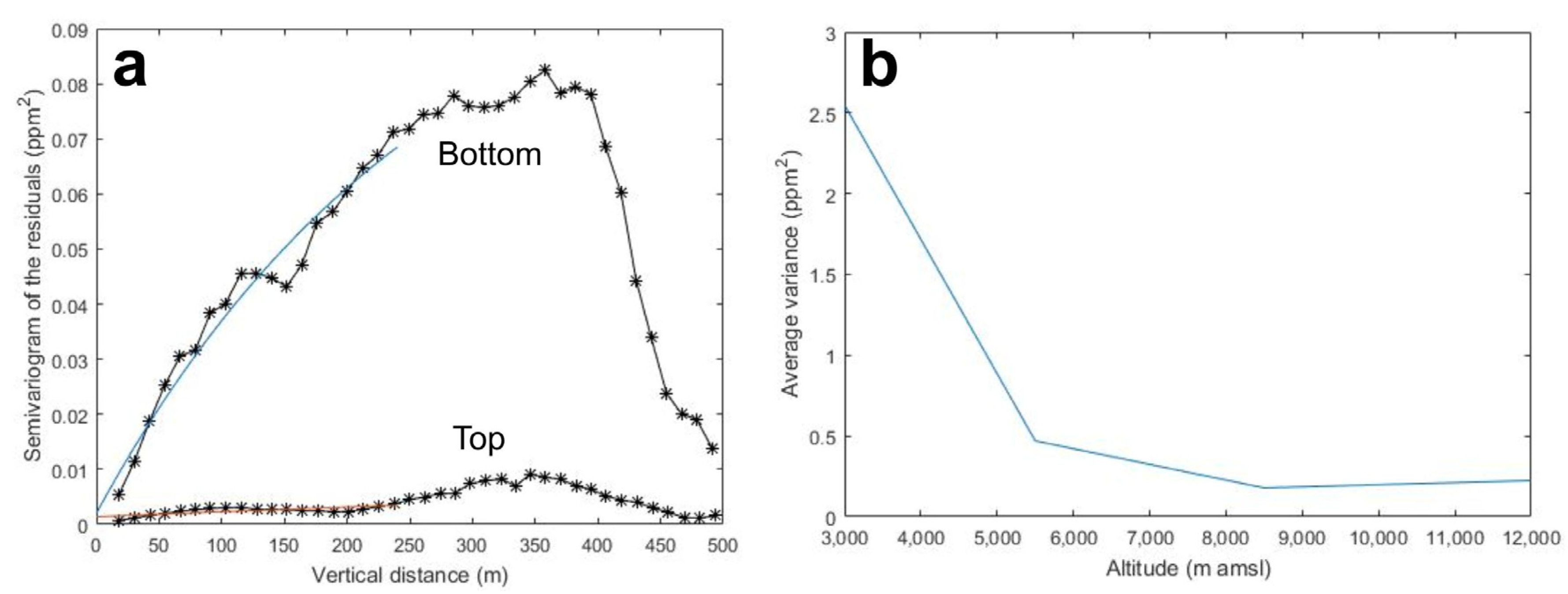
3.1. Covariance Model Selection and Local Parameter Inference

Figure 1 shows: (a) a semi-variogram of the residuals as a function of the vertical distance and (b) its average variance as a function of elevation. From Figure 1, it follows that the modeled profiles tend to better represent observed variability at higher altitudes, and show smaller model/data mismatches. This indirectly supports one of the initial assumptions of our approach: to impose the collapse of the residuals at the top of the atmosphere. The differences in variograms at the top and bottom of the atmospheric profile confirm non-stationarity of the covariance, and emphasize the need to implement a moving window approach. Variograms were separately modeled for each CO2 and CH4 in situ sampling simulation.

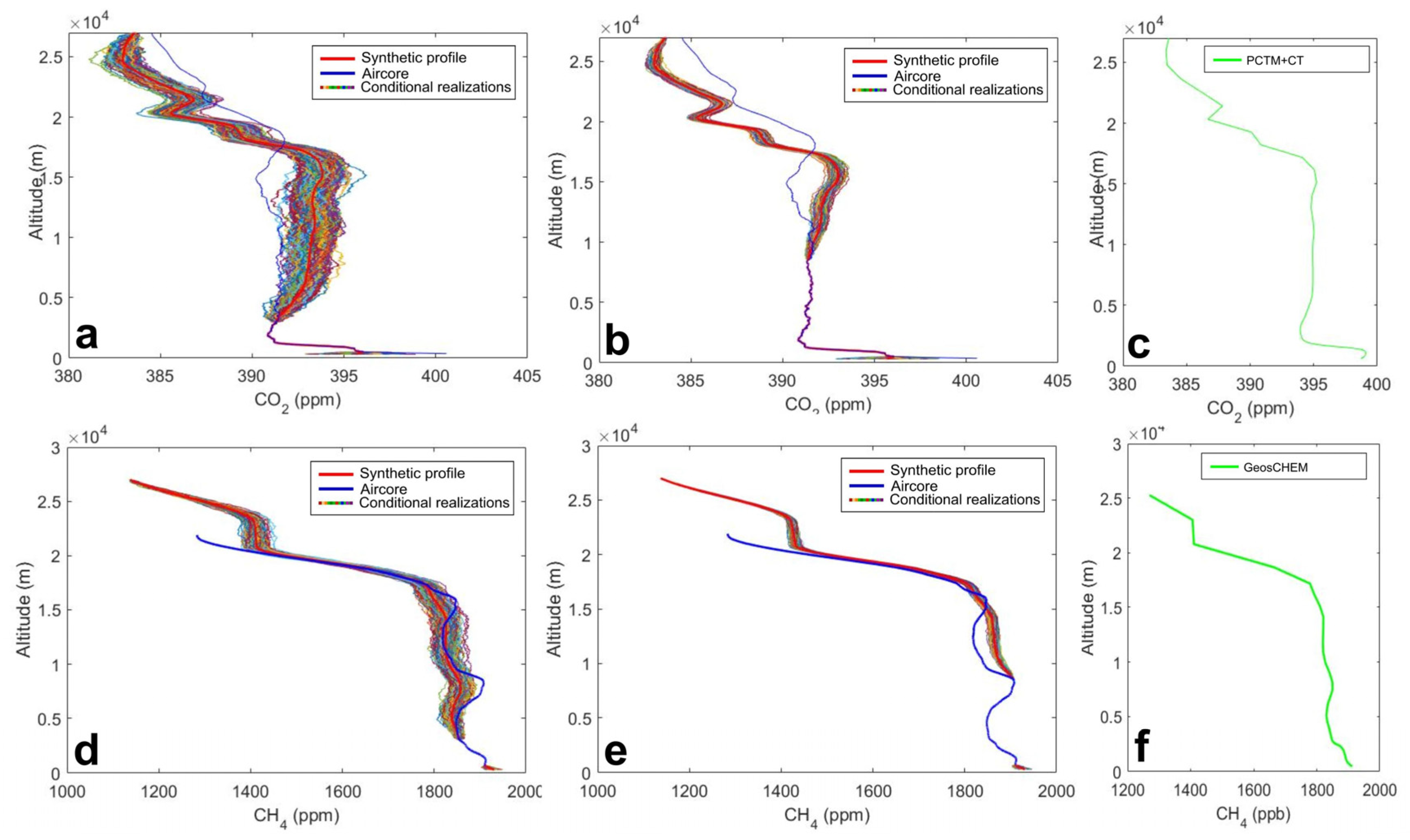
3.2. Simulation of the Full-Column (Synthetic) Profiles

3.2.1. Scenario 1: Partial Column Profiles Available

Figure 2 shows synthetic vertical profiles obtained following our approach.
In Supporting Information, Tables S1 and S3, we show detailed results for each site for a total of 14 sites. Although PCTM profiles significantly overestimate XCO2, and GEOS-Chem underestimates XCH4 total column values compared to observed AirCore vertical profiles, our approach, by design, removes this mismatch at sampled locations, which can be viewed as some sort of shifting. Thus, our individual synthetic vertical profile is a closer match to the observed vertical profile. The ability of the synthetic vertical profiles to match the observed vertical profiles will depend on the accuracy of the modeled vertical profiles, and specifically on realistic representation of the vertical variability. In the case of CH4 whose concentration drastically decreases in the stratosphere, the accuracy of synthetic vertical CH4 profiles will depend on how accurately the model simulates a tropopause height (this problem also affects CO2 to a lesser extent). Given this limitation, the altitude range of observations required to equally constrain total column estimates are dependent on the factors that affect accuracy in estimating tropopause height, e.g., latitude, location, and season. This weakness should diminish as both Atmospheric Transport Model (ATM) accuracy and our approach co-evolve.

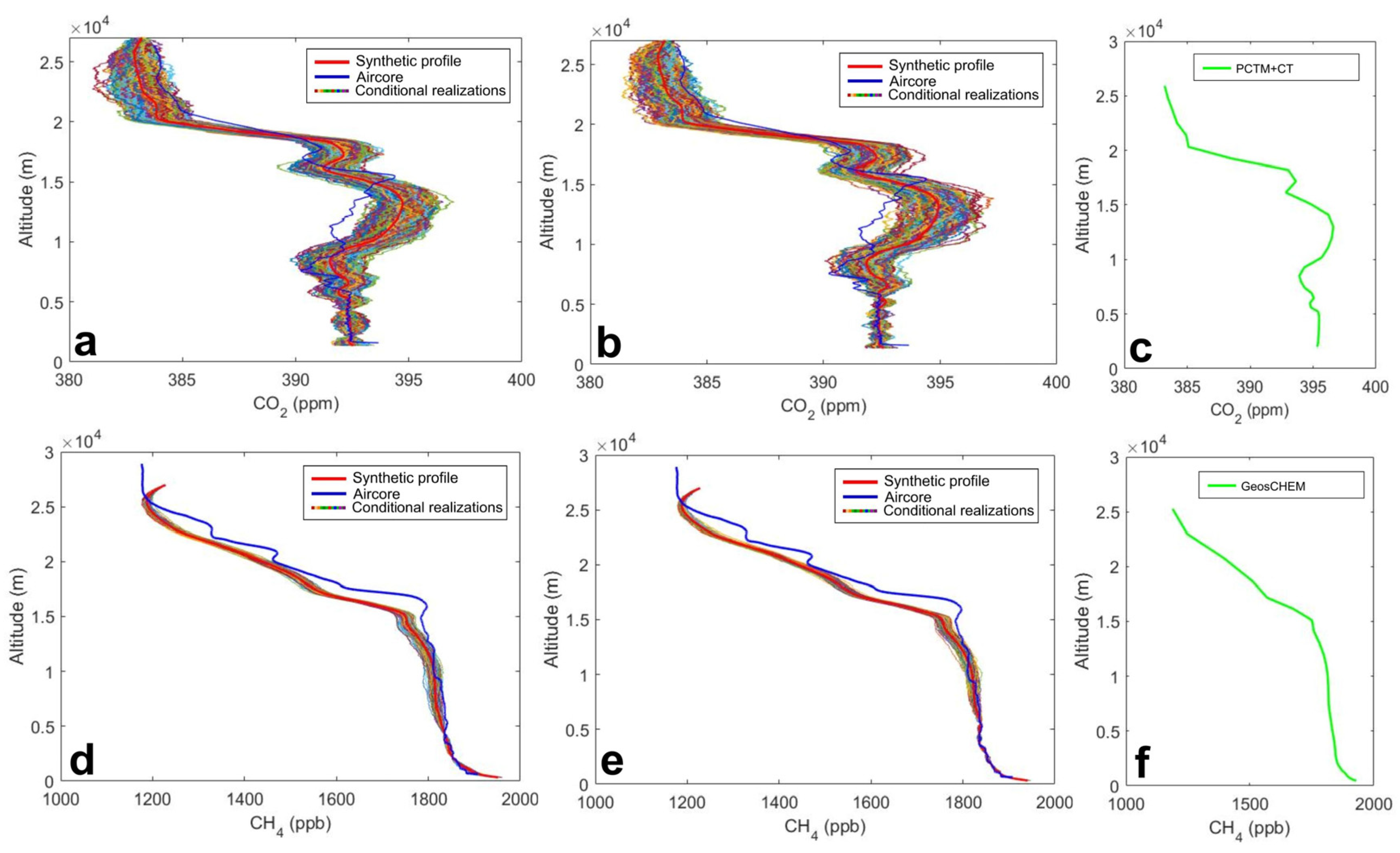
3.2.2. Scenario 2: Only Discrete Profiles Available

In the case of discrete (i.e., flask) vertical profiles, the covariance structure of the residuals cannot be determined due to insufficient information from observations. Insufficient number of sampled points, and the fact that samples are often nearly equi-spaced, prevent observing the dependence of the semi-variance with distance, which is necessary for inferring the covariance structure. In this case, we imposed average observed covariance parameters on the entire dataset, and reconstructed missing fractions of the column using a few measurement points (flasks). Results are shown in Figure 3 and Supporting Information Tables S2 and S4.

3.3. Uncertainty Analysis and Potential Method Applicability

Proper uncertainty analysis assumes understanding the uncertainty that stems from both deterministic and stochastic components of the synthetic vertical profiles, and then comparing the synthetic and observed vertical profiles.
Estimating the missing part of the vertical profile through conditional realizations was intended as a way to assess the precision of the total column estimates. However, in this case the precision based on ensemble conditional realizations is not a realistic representation of the true error statistics. The residual kriging approach, by our study’s design, assumes that the relationship between corrected modeled vertical profiles (model + residuals) at the sampled range of altitudes will hold for an unsampled fraction of the column. This is wrong, as the ‘model + residuals’ is set to be equivalent to sampled altitudes, while it is not true for the unsampled fraction of the column. Thus, the variance of XCO2 estimates derived from column profiles based on ensemble conditional realizations should be added to the unknown variance stemming from the inability of the combined ‘model + residuals’ profile (which provides the drift) to hold the same relationship to the true vertical profile at unsampled altitudes. A realistic error analysis based on the comparison between total column values derived from synthetic and AirCore vertical profiles is shown in Table 1.
At the time of study, the number of available AirCore observations globally was 14. Given the relatively small sample number (14) and missing information about the true standard deviation in the error population mean, we used a two-tailed t-statistics (not z-statistics) method to assess the uncertainty bounds of error estimates, and determined that the minimum sample size required for the study was eight. We rephrased the common question in t-statistics test and checked how far away the true error in the mean has to be to still fall into 95% confidence interval for each of the examined scenarios (Table 1).
Error analysis revealed a few interesting properties of our approach. First, the method based on the PCTM and GEOS-Chem models has its own bias, and tends to overestimate XCO2 by ~0.3 ppm. A bias correction generally improves the error statistics. In Table 1, we show both unbiased (bias-corrected) and uncorrected standard deviations of XCO2 values derived from the synthetic vertical profiles (bias correction was done by shifting the mean, and given that errors are not normally distributed with outliers, in a few cases the error was increased by shifting the mean).

3.4. Comparison with TCCON Retrievals

A comparison of direct measurements of the atmosphere and TCCON indicates a correction of 0.989 ± 0.002 is needed for XCO2, and 0.978 ± 0.004 for XCH4 [5], given as the ratio between aircraft and TCCON-derived profiles (2σ). Apart from implying a need for a constant TCCON calibration to maintain its accuracy at the desired level, the reported precision translates into ~0.8 ppm 2σ uncertainty for a baseline CO2 mixing ratio of 400 ppm, and 8 ppb for CH4, given 2000 ppb baseline mole fraction. Geibel et al. (2012) [8] found that the average correction for TCCON XCH4 needed to match the aircraft observations was −7 ppb. (Note: there can be residual bias in TCCON retrievals due to temporal sparsity of calibrations, but we do not further analyze these biases here. For a detailed recent analysis of TCCON uncertainty please see Inoue et al., 2016 [41]).
One of the goals of our study is to assess the minimum flight altitude required for the synthetic profile derived for XCO2 to achieve uncertainty close to TCCON’s. Table 1 shows that one would have to fly at least to 9000–9500 m using a non-bias-corrected method. However, this changes after correcting for bias; that result shows that flights up to ~6000 m, in combination with our approach, could yield an XCO2 total column estimate with error statistics comparable to TCCON. For XCH4, both continuous and flask sampling in combination with profiles fail to match the reported uncertainty of TCCON.

3.5. Conceptual Comparison to Classical Approach

One interesting feature of our approach (Table 1) is that the total column MAE obtained by sampling continuously up to 3000 m is slightly larger than having a single flask sample at 3250 m. This result may appear counterintuitive. In the classical approach, sampling a wider range of altitudes (i.e., flying higher) necessarily means better constraining the total column estimate. This logic is generally the case, but several complications can produce unexpected results, like the result described above. In these cases, the location where flask samples are collected within the vertical profile can be as important as the total number of flask samples. Furthermore, the accuracy of the atmospheric model (i.e., auxiliary information) can be more important at some altitudes than others.
Figure 4 displays the results of a thought experiment and is one illustrative example of this challenge. In this thought experiment, we assume a specific true vertical profile of CO2 (Figure 4a). We also assume that the modeled vertical profile nearly perfectly reflects the variability of the observed vertical profile, except between ~10–16 km altitude. Furthermore, in our thought experiment, the model has a positive offset ~2 ppm at lower altitudes (Figure 4b). We also assume two cases having a continuous sampling up to 10 km (Figure 4c), and 14 km (Figure 4d).
We constructed a full XCO2 column using these synthetic vertical profiles, and observed several interesting features. In the first case, the atmospheric model (i.e., auxiliary information) affects the shape of the synthetic vertical profile at altitudes where the atmospheric model exhibits deviations from the truth, but not significantly above that range of altitudes. However, in the case of simulated sampling up to 14 km, the deviations of the model negatively affect the synthetic vertical profile at the entire range of altitudes above the observed fraction. In the latter case, the retrieved total column estimate is less accurate that in the first case, although the sampling covers a wider range of altitudes. This result shows that, in our approach, a large sampling domain is important, but the accuracy of the synthetic vertical profiles is also dependent on how well the atmospheric model reproduces the observed vertical profile at the highest observed altitude. Atmospheric models generally tend to be more accurate at higher altitudes where mixing ratios are less heterogeneous and inaccuracies in estimated surface fluxes have less of an effect. In this specific thought experiment, the subtle interplay between inaccurate representations of the variability by the atmospheric transport model and the absolute accuracy of the model results in having high altitude discrete observations which do not correct or nudge the atmospheric model in a way that improves accuracy across the entire column.

4. Conclusions

In this paper, we present an alternative approach to estimating XCO2 using partial column observations and external sources of information. We demonstrate and evaluate the method by creating synthetic vertical profiles at several sites where AirCore observations are available, which we used as true vertical profiles. We assess the reliability of the error statistics based on the analysis of ensemble conditional simulations and true differences between synthetic and AirCore vertical profiles, and conclude that the spread in conditional realizations and corresponding total column estimates cannot be used to realistically represent the true error statistics.
The statistics based on the comparison to AirCore vertical profiles show that a level of precision comparable to that of TCCON can be achieved by using a non-biased version of our approach and flights up to ~6000 m amsl (for ground elevations <~1500 m like at the AirCore sites) using PCTM modeled derived vertical profiles. We show that by combining the modeled vertical profile, the model-specific assigned variability, and in situ observations, the number of equidistant flasks could be reduced to as low as two in the 0–6500 m amsl range, while still retaining the ability to estimate total column values at a level of accuracy comparable to those achieved using continuous airborne-based observations. The findings of this study is in contradiction to the conclusion from [13], which shows having less than 8–10 flask samples leads to a degradation of the information content for some common CO2 vertical profiles.
Note that the limited number of available AirCore observations reduced the number of CO2 vertical profiles examined in this paper. Derived error statistics for the overall performance of the two models might have been affected by the non-representativeness of the performance of models at 14 sites where AirCore vertical profiles are available. Unfortunately, using models of aircraft vertical profiles as AirCore surrogates in this study is ruled out, as model-to-model differences exceed the model-to-truth differences and will likely affect the error statistics when aircraft vertical profiles exhibit non-negligible effects of the superposition of horizontal and vertical variability [36].
While we used the PCTM and GEOS-Chem chemical transport models (CTMs) in this study, our conceptual approach goes beyond selection of any particular source of external information: it tries to establish a new paradigm in creating synthetic vertical profiles based on limited information from samples and auxiliary information. In fact, as global knowledge and observational coverage increase, and thus the reliability of auxiliary information, the resulting synthetic vertical profile will continually become closer to the true value.
A few factors can adversely affect the reliability of this extrapolation method. In this study, we sampled AirCore vertical profiles in a manner consistent with continuous or discrete observations of the partial column. Therefore, the accuracy of the sampled vertical profile was as accurate as the AirCore vertical profiles themselves. In fact, AirCore vertical profiles were imposed as a truth for the purpose of this study. In practice, observations are collected from airborne platforms, which may capture partial vertical profiles, or from use of flasks, which has an intrinsic uncertainty that has to be accounted for.
We envision that further improvements in the quality of the modeled vertical profiles, either through better understanding of the physico-chemical processes that affect their shapes, or simply by assimilating more observations, will push these threshold altitudes down to ranges reachable even by commercially available small unmanned aerial vehicles (UAVs) (3000–4000 m) (e.g., https://www.microdrones.com/en/products/md4-3000/). Besides the maximum altitude, the biggest limitations for current UAVs are their limited payload (a few kg) and flight endurance (30 min). We provide evidence that a few flask samples collected at optimal altitudes can yield accurate XCO2 estimates, which, in combination with further development of small UAVs instrumented with lightweight flask sampling systems, could open possibilities of getting XCO2 estimates at low cost, while achieving accuracy comparable to expensive, labor intensive TCCON-based XCO2.

Supplementary Materials

The following are available online at https://www.mdpi.com/2073-4433/9/7/247/s1, Table S1: Estimated total column (XCO2) values (ppm) derived from AirCore, model-only (PCTM + CarbonTracker (CT)) and synthetic vertical profiles calculated using our approach based on partial, Table S2: Estimated total column (XCO2) values (ppm) derived from AirCore vertical profiles, different number of simulated flask samples taken at 0–6500 m amsl altitude range, and model-only (PCTM + CarbonTracker (CT)), Table S3: Estimated total column (XCH4) values (ppm) derived from AirCore vertical profiles, modelonly (GEOS-Chem) and synthetic vertical profiles, calculated using our approach based on partial column measurements, Table S4: Estimated total column (XCH4) values (ppm) derived from AirCore vertical profiles, different number of simulated flask samples taken at 0–6500 m amsl altitude range, and model-only (GEOS-Chem) column measurements.

Author Contributions

J.M.T. and S.C.B. conceived and designed the experiments; J.M.T. performed the experiments; J.M.T. and S.C.B. analyzed the data and wrote the paper.

Funding

This work was supported by the Office of Biological and Environmental Research of the US Department of Energy under contract No. DE-AC02-05CH11231 as part of the Atmospheric Radiation Measurement Program (ARM), ARM Aerial Facility (AAF), and Terrestrial Ecosystem Science Program (TES).

Acknowledgments

We thank Scot Miller (Carnegie Institution for Science, Department for Global Ecology) for providing the modeled vertical profiles used in this study, and Colm Sweeney (National Oceanic and atmospheric Administration, Global monitoring Division) for providing AirCore vertical profiles. All data used in this study are available upon request.

Conflicts of Interest

The authors declare no conflict of interest.

Appendix A

Residual (Regression) Kriging

The modeling procedure followed several steps. First, we calculate a raw variogram of the residuals based on the observations falling within the predefined window:
γ ( h ) = 1 2 [ y ( x i ) y ( x j ) ] 2
where γ is the raw variogram value for a given pair of residuals y(xi) and y(xj), and h is the vertical distance between the locations ( x i and x j ) of these residuals.
Second, the theoretical variogram is fitted to the raw variogram using non-linear least squares. We chose an exponential variogram function with a nugget effect, based upon visual inspection of variograms:
γ ( h ) = { 0 ,   f o r   h = 0 σ 2 ( 1 exp ( h l ) ) + σ n u g 2 ,   f o r   h > 0
where σ2 and l are the variance and correlation length of the quantity being mapped, and σ2nug is the nugget variance, typically representative of measurement errors and very close to zero in this study.
Under the second-order stationarity assumption, covariance and semi-variogram can be regarded as equivalent statistical tools, as there is a simple relation between them:
γ(h) = C(0) − C(h)
where h is the distance between points, and C(0) is “sill” (semivariogram value at infinite distance).
The typical semi-variogram of the residuals at the top and bottom fractions of the sampled portion of the column is shown in Figure 1.
The variogram parameters can be used to define a corresponding local spatial covariance structure (q). For the variogram function in Equation (A2), this becomes:
q ( h ) = σ 2 exp ( h l )
Third, the linear system of equations that is solved to obtain the N weights λ assigned to the residuals within a predefined window:
  [ Q + R 1 1 T 0 ] [ λ ν ] = [ q 0 1 ]
where Q is an N × N covariance matrix among the N residuals with individual entries as defined in Equation (A3), R is an N × N diagonal measurement and retrieval error covariance matrix among the N residuals, 1 is an N × 1 unity vector, T denotes the vector transpose operation, and q0 is an N × 1 vector of the spatial covariances between the estimation locations and the N locations of residuals.
The system in Equation (A5) is solved for λ and the Lagrange multiplier ν . These parameters are then used to define the estimate (ẑ) and estimation uncertainty variance (σ2) for the estimation location as:
ẑ= λTy
σ2 = σ0λT qA + ν
where y is the N × 1 vector of subsampled observations, and σ0 is the variance of the residuals.
All calculations were conducted in a Euclidean coordinate system, while AirCore and modeled profile coordinates were given in Lat/Long/Alt format based on WGS84 spheroid earth model [42]. The coordinates were converted into the Universal Transverse Mercator coordinate system to allow computations of distances and angles using Euclidean geometry over short distances [43].

Appendix B

Conditional Simulations

Conditional realizations (also known as spatially-consistent Monte Carlo simulations) of CH4 and CO2 variability were generated for every test case, extending from the highest sampled altitude to 1 hPa. They represent equally probable realizations of a spatial random function. Each realization honors both observed values at measurement locations and imposed reduction in the variability of the model/measurement mismatch with altitude. Conditional simulations could be viewed as being based on both the data and the model, and consistent with observed values and with the degree of variability expected of the true (unknown) distribution of the model/data mismatch. Individually, the conditional realizations provide an accurate representation of the degree of variability in the unknown “true” field, while the average across conditional realizations asymptotically approaches the kriging estimate as the number of realizations tends to infinity. The ensemble of conditional realizations represents the uncertainty in the estimated profile that stems from the stochastic component of the synthetic profile. Conditional realizations differ from kriging, which provides point-wise “best estimates,” but kriging estimates are spatially smoother than reality.
We generated an ensemble of 200 conditional simulations for each test case (each available AirCore profile). Each realization (sci, m × 1) was calculated as (see [44] for additional details):
sci = Λ(zzui) + sui
where Λ is the m × n matrix of weights defined in Equation (A4), z (n × 1) are the observations, and zui (n × 1) and sui (m × 1) are unconditional realizations at measurement (n) and estimation (m) locations, respectively, obtained from:
  [ z u i s u i ] = C T u
where u is an (n + m) × 1 vector of normally distributed random values with zero mean and unit variance (a new vector u is generated for each realization), and C is the (n + m) × (n + m) matrix resulting from the Cholesky decomposition of the covariance matrix:
  [ Q + R 1 1 T 0 ] = C C T
The vector components of the matrix Λ used in Equation (A8) ( λ ) , and Lagrange multipliers are obtained by solving the system of linear equations shown in Equation (A5) (see examples of the generated conditional realizations in Figure 2).

References

  1. Miyamoto, Y.; Inoue, M.; Morino, I.; Uchino, O.; Yokota, T.; Machida, T.; Sawa, Y.; Matsueda, H.; Sweeney, C.; Tans, P.P.; et al. Atmospheric column-averaged mole fractions of carbon dioxide at 53 aircraft measurement sites. Atmos. Chem. Phys. 2013, 13, 5265–5275. [Google Scholar] [CrossRef]
  2. Tadić, J.M.; Loewenstein, M.; Frankenberg, C.; Butz, A.; Roby, M.; Iraci, L.T.; Yates, E.L.; Gore, W.; Kuze, A. A comparison of in-situ aircraft measurements of carbon dioxide and methane to GOSAT data measured over Railroad Valley playa, Nevada, USA. IEEE Trans. Geosci. Remote Sens. 2014, 52, 7764–7774. [Google Scholar] [CrossRef]
  3. Tanaka, T.; Miyamoto, Y.; Morino, I.; Machida, T.; Nagahama, T.; Sawa, Y.; Matsueda, H.; Wunch, D.; Kawakami, S.; Uchino, O. Aircraft measure-ments of carbon dioxide and methane for the calibration of ground-based high-resolution Fourier Transform Spectrometers and a comparison to GOSAT data measured over Tsukuba and Moshiri. Atmos. Meas. Tech. 2012, 5, 2003–2012. [Google Scholar] [CrossRef]
  4. Inoue, M.; Morino, I.; Uchino, O.; Miyamoto, Y.; Yoshida, Y.; Yokota, T.; Machida, T.; Sawa, Y.; Matsueda, H.; Sweeney, C.; et al. Validation of XCO2 derived from SWIR spectra of GOSAT TANSO-FTS with aircraft measurement data. Atmos. Chem. Phys. 2013, 13, 9771–9788. [Google Scholar] [CrossRef]
  5. Wunch, D.; Toon, G.C.; Blavier, J.-F.L.; Washenfelder, R.A.; Notholt, J.; Connor, B.J.; Griffith, D.W.T.; Sherlock, V.; Wennberg, P.O. The Total Carbon Column Observing Network. Phil. Trans. R. Soc. A 2011, 369, 2087–2112. [Google Scholar] [CrossRef] [PubMed] [Green Version]
  6. Messerschmidt, J.; Geibel, M.C.; Blumenstock, T.; Chen, H.; Deutscherm, N.M.; Engel, A.; Feist, D.G.; Gerbig, C.; Gisi, M.; Hase, F.; et al. Calibration of TCCON column-averaged CO2: The first aircraft campaign over European TCCON sites. Atmos. Chem. Phys. 2011, 11, 10765–10777. [Google Scholar] [CrossRef]
  7. Deutscher, N.M.; Griffith, D.W.T.; Bryant, G.W.; Wennberg, P.O.; Toon, G.C.; Washenfelder, R.A.; Keppel-Aleks, G.; Wunch, D.; Yavin, Y.; Allen, N.; et al. Total column CO2 measurements at Darwin, Australia—Site description and calibration against in situ aircraft profiles. Atmos. Meas. Tech. 2010, 3, 947–958. [Google Scholar] [CrossRef]
  8. Geibel, M.C.; Messerschmidt, J.; Gerbig, C.; Blumenstock, T.; Chen, H.; Hase, F.; Kolle, O.; Lavrič, J.V.; Notholt, J.; Palm, M.; et al. Calibration of column-averaged CH4 over European TCCON FTS sites with airborne in-situ measurements. Atmos. Chem. Phys. 2012, 12, 8763–8775. [Google Scholar] [CrossRef]
  9. Biraud, S.C.; Torn, M.S.; Smith, J.R.; Sweeney, C.; Riley, W.J.; Tans, P.P. A multi-year record of airborne CO2 observations in the US Southern Great Plains. Atmos. Meas. Tech. 2013, 6, 751–763. [Google Scholar] [CrossRef]
  10. Inoue, M.; Morino, I.; Uchino, O.; Miyamoto, Y.; Saeki, T.; Yoshida, Y.; Yokota, T.; Sweeney, C.; Tans, P.P.; Biraud, S.C.; et al. Validation of XCH4 derived from SWIR spectra of GOSAT TANSO-FTS with aircraft measurement data. Atmos. Meas. Tech. 2014, 7, 2987–3005. [Google Scholar] [CrossRef]
  11. O’Dell, C.W.; Connor, B.; Bösch, H.; O’Brien, D.; Frankenberg, C.; Castano, R.; Christi, M.; Eldering, D.; Fisher, B.; Gunson, M.; et al. The ACOS CO2 retrieval algorithm—Part 1: Description and validation against synthetic observations. Atmos. Meas. Tech. 2012, 5, 99–121. [Google Scholar] [CrossRef]
  12. Foucher, P.Y.; Chedin, A.; Armante, R.; Boone, C.; Crevoisier, C.; Bernath, P. Carbon dioxide atmospheric vertical profiles retrieved from space observation using ACE-FTS solar occultation instrument. Atmos. Chem. Phys. 2011, 11, 2455–2470. [Google Scholar] [CrossRef] [Green Version]
  13. Bakwin, P.S.; Tans, P.P.; Stephens, B.B.; Wofsy, S.C.; Gerbig, C.; Grainger, A. Strategies for measurement of atmospheric column means of carbon dioxide from aircraft using discrete sampling. J. Geophys. Res. 2003, 108, 4514. [Google Scholar] [CrossRef]
  14. Karion, A.; Sweeney, C.; Tans, P.; Newberger, T. AirCore: An Innovative Atmospheric Sampling System. J. Atmos. Ocean. Tech. 2010, 27, 1839–1853. [Google Scholar] [CrossRef]
  15. Membrive, O.; Crevoisier, C.; Sweeney, C.; Danis, F.; Hertzog, A.; Engel, A.; Bönisch, H.; Picon, L. AirCore-HR: A high-resolution column sampling to enhance the vertical description of CH4 and CO2. Atmos. Meas. Tech. 2017, 10, 2163–2181. [Google Scholar] [CrossRef]
  16. Kawa, S.R.; Erickson, D.J.; Pawson, S.; Zhu, Z. Global CO2 transport simulations using meteorological data from the NASA data assimilation system. J. Geophys. Res. 2004, 109. [Google Scholar] [CrossRef]
  17. Pickett-Heaps, C.A.; Jacob, D.J.; Wecht, K.J.; Kort, E.A.; Wofsy, S.C.; Diskin, G.S.; Worthy, D.E.J.; Kaplan, J.O.; Bey, I.; Drevet, J. Magnitude and seasonality ofwetland methane emissions from the Hudson Bay Lowlands (Canada). Atmos. Chem. Phys. 2011, 11, 3773–3779. [Google Scholar] [CrossRef] [Green Version]
  18. Wecht, K.J.; Jacob, D.J.; Wofsy, S.C.; Kort, E.A.; Worden, J.R.; Kulawik, S.S.; Henze, D.K.; Kopacz, M.; Payne, V.H. Validation of TES methane with HIPPO aircraft observations: Implications for inverse modeling of methane sources. Atmos. Chem. Phys. 2012, 12, 1823–1832. [Google Scholar] [CrossRef] [Green Version]
  19. Turner, A.J.; Jacob, D.J.; Wecht, K.J.; Maasakkers, J.D.; Lundgren, E.; Andrews, A.E.; Biraud, S.C.; Boesch, H.; Bowman, K.W.; Deutscher, N.M.; et al. Estimating global and North American methane emissions with high spatial resolution using GOSAT satellite data. Atmos. Chem. Phys. 2015, 15, 7049–7069. [Google Scholar] [CrossRef] [Green Version]
  20. Rienecker, M.M.; Suarez, M.J.; Gelaro, R.; Todling, R.; Bacmeister, J.; Liu, E.; Bosilovich, M.G.; Schubert, S.D.; Takacs, L.; Kim, G.K.; et al. MERRA: NASA’s modern-era retrospective analysis for research and applications. J. Clim. 2011, 24, 3624–3648. [Google Scholar] [CrossRef]
  21. Peters, W.; Jacobson, A.R.; Sweeney, C.; Andrews, A.E.; Conway, T.J.; Masarie, K.; Miller, J.B.; Bruhwiler, L.M.P.; Petron, G.; Hirsch, A.I.; et al. An atmospheric perspective on North American carbon dioxide exchange: CarbonTracker. Proc. Natl. Acad. Sci. USA 2007, 104, 18925–18930. [Google Scholar] [CrossRef] [PubMed] [Green Version]
  22. CarbonTracker CT2017. Available online: https://www.esrl.noaa.gov/gmd/ccgg/carbontracker/ (accessed on 22 June 2018).
  23. Wecht, K.J.; Jacob, D.J.; Frankenberg, C.; Jiang, Z.; Blake, D.R. Mapping of North American methane emissions with high spatial resolution by inversion of SCIAMACHY satellite data. J. Geophys. Res. Atmos. 2014, 119, 7741–7756. [Google Scholar] [CrossRef] [Green Version]
  24. Bruhwiler, L.; Dlugokencky, E.; Masarie, K.; Ishizawa, M.; Andrews, A.; Miller, J.; Sweeney, C.; Tans, P.; Worthy, D. CarbonTracker-CH4: An assimilation system for estimating emissions of atmospheric methane. Atmos. Chem. Phys. 2014, 14, 8269–8293. [Google Scholar]
  25. Trends in Global CO2 Emissions: 2015 Report. Available online: http://edgar.jrc.ec.europa.eu/news_docs/jrc-2015-trends-in-global-co2-emissions-2015-report-98184.pdf (accessed on 22 June 2018).
  26. Van der Werf, G.R.; Randerson, J.T.; Giglio, L.; Collatz, G.J.; Mu, M.; Kasibhatla, P.S.; Morton, D.C.; DeFries, R.S.; Jin, Y.; van Leeuwen, T.T. Global fire emissions and the contribution of deforestation, savanna, forest, agricultural, and peat fires (1997–2009). Atmos. Chem. Phys. 2010, 10, 11707–11735. [Google Scholar] [CrossRef] [Green Version]
  27. Akagi, S.K.; Yokelson, R.J.; Wiedinmyer, C.; Alvarado, M.J.; Reid, J.S.; Karl, T.; Crounse, J.D.; Wennberg, P.O. Emission factors for open and domestic biomass burning for use in atmospheric models. Atmos. Chem. Phys. 2011, 11, 4039–4072. [Google Scholar] [CrossRef]
  28. File Specification for GEOS-5 FP. GMAO Office Note No. 4 (Version1.0). 2013. Available online: http://acmg.seas.harvard.edu/geos/wiki_docs/geos5/GEOS_5_FP_File_Specification_ON4v1_0.pdf (accessed on 22 June 2018).
  29. CarbonTracker-CH4. Available online: https://www.esrl.noaa.gov/gmd/ccgg/carbontracker-ch4/ (accessed on 22 June 2018).
  30. Hengl, T.; Geuvelink, G.B.M.; Stein, A. Comparison of Kriging with External Drift and Regression-Kriging. Technical Note, ITC. 2003. Available online: https://webapps.itc.utwente.nl/librarywww/papers_2003/misca/hengl_comparison.pdf (accessed on 22 June 2018).
  31. Haas, T.C. Lognormal and moving window methods of estimating acid deposition. J. Am. Stat. Assoc. 1990, 85, 950–963. [Google Scholar] [CrossRef]
  32. Laiti, L.; Zardi, D.; de Franceschi, M.; Rampanelli, G. Residual Kriging analysis of airborne measurements: Application to the mapping of Atmospheric Boundary-Layer thermal structures in a mountain valley. Atmos. Sci. Lett. 2013, 14, 79–85. [Google Scholar] [CrossRef]
  33. Chiles, J.-P.; Delfiner, P. Geostatistics, 2nd ed.; Wiley: Hoboken, NJ, USA, 2012. [Google Scholar]
  34. Holdaway, M.R. Spatial modeling and interpolation of monthly temperature using kriging. Clim. Res. 1996, 6, 215–225. [Google Scholar] [CrossRef] [Green Version]
  35. Tadić, J.M.; Ilić, V.; Biraud, S. Examination of geostatistical and machine-learning techniques as interpolators in anisotropic atmospheric environments. Atmos. Environ. 2015, 111, 28–38. [Google Scholar] [CrossRef] [Green Version]
  36. Tadić, J.M.; Michalak, A.M. On the effect of spatial variability and support on validation of remote sensing observations of CO2. Atmos. Environ. 2016, 132, 309–316. [Google Scholar] [CrossRef]
  37. Ahmed, S.; de Marsily, G. Comparison of geostatistical methods for estimating transmissivity using data on transmissivity and specific capacity. Water Resour. Res. 1987, 23, 1717–1737. [Google Scholar] [CrossRef]
  38. Hengl, T.; Heuvelink, G.B.M.; Rossiter, D.G. About regression-kriging: From equations to case studies. Comput. Geosci. 2007, 33, 1301–1315. [Google Scholar] [CrossRef]
  39. Sweeney, C.; Karion, A.; Wolter, S.; Newberger, T.; Guenther, D.; Higgs, J.A.; Andrews, A.E.; Lang, P.M.; Neff, D.; Dlugokencky, E.; et al. Seasonal climatology of CO2 across North America from aircraft measurements in the NOAA/ESRL Global Greenhouse Gas Reference Network. J. Geophys. Res. Atmos. 2015, 120, 5155–5190. [Google Scholar] [CrossRef]
  40. Tans, P.P.; Bakwin, P.S.; Guenther, D.W. A feasible global carbon cycle observing system: A plan to decipher today’s carbon cycle based on observations. Glob. Chang. Biol. 1996, 2, 309–318. [Google Scholar] [CrossRef]
  41. Inoue, M.; Morino, I.; Uchino, O.; Nakatsuru, T.; Yoshida, Y.; Yokota, T.; Wunch, D.; Wennberg, P.O.; Roehl, C.M.; Griffith, D.W.T.; et al. Bias corrections of GOSAT SWIR XCO2 and XCH4 with TCCON data and their evaluation using aircraft measurement data. Atmos. Meas. Tech. 2016, 9, 3491–3512. [Google Scholar] [CrossRef]
  42. The Earth Model—Calculating Field Size and Distances between Points Using GPS Coordinates. Available online: http://www.ipni.net/publication/ssmg.nsf/0/0BDF314BF75B9FC1852579E5007691F9/$FILE/SSMG-11.pdf (accessed on 22 June 2018).
  43. Li, J.; Heap, A. A Review of Spatial Interpolation Methods for Environmental Scientists; Geoscience Australia: Canberra, Australia, 2008; p. 137. [Google Scholar]
  44. Zhou, Y.; Obenour, D.R.; Scavia, D.; Johengen, T.H.; Michalak, A.M. Spatial and temporal trends in Lake Erie hypoxia, 1987–2007. Environ. Sci. Technol. 2013, 47, 899–905. [Google Scholar] [CrossRef] [PubMed]
Figure 1. (a) Example variograms of the residuals at 200 and 8500 m altitude (window size ±500 m) for CO2 (01/14/2012); (b) Height dependence of the average estimated variance for CO2 of the residuals (window size ±500 m) for the entire dataset.
Atmosphere 09 00247 g001
Figure 2. Sampled and reconstructed fraction of the CO2 column (24 October 2012) (a,b), and CH4 (17 September 2014) (d,e) showing ensemble conditional realization cloud based on the covariance parameters inferred at the top of the sampled partial column. Modeled profiles for CO2 and CH4 are given in (c,f), respectively. Red line extending from the top of the sampled fraction upward represents the synthetic profile. Simulated sampled column altitude range was: (a) h < 3000 m and (b) h < 8500 m, visible in the profiles as the altitude ranges where conditionally simulated ensembles are missing.
Atmosphere 09 00247 g002
Figure 3. Reconstructed full vertical CO2 (a,b) (15 August 2012) and CH4 (d,e) (15 January 2012) profiles showing ensemble conditional realization cloud based on the imputed covariance parameters (sill 0.41 ppm2 and 55 ppb2, range parameter 6000 m and 10,000 m, for CO2 and CH4, respectively). Modeled profiles for CO2 and CH4 are given in (c,f), respectively. Red line represents the mean of 200 conditional realizations and the reconstructed full profile shape. The number of simulated flasks shown was two for (a,c), and six for (c,d).
Atmosphere 09 00247 g003
Figure 4. Depiction of the key elements of a thought experiment: (a) assumed true profile; (b) assumed modeled profile; (c) true and reconstructed profile assuming sampling up to 10 km; and (d) assumed true and reconstructed profile assuming sampling up to 14 km.
Atmosphere 09 00247 g004
Table 1. Error statistics for total column CO2 (XCO2) and CH4 (XCH4) based on simulated partial profiles and flask sampling given as mean absolute error (MAE; ppm), standard deviation from the true value (AirCore derived total column), and standard deviation in an “unbiased scenario” where the XCO2 mean of synthetic profile and the true value are the same. The confidence interval was derived from two-tailed t-statistics.
Greenhouse GasParametersPartial Profiles (<m amsl)Number of Flasks, 0–6500 m
3000550065007500850012612
CO2MAE (ppm)0.760.500.370.360.320.600.440.490.51
95% MAE confidence interval0.410.250.170.160.120.340.200.180.25
σ (ppm)0.930.660.500.480.440.690.540.690.66
Unbiased σ (ppm)0.600.440.360.350.340.450.420.540.45
CH4MAE (ppb)7.727.678.611.239.858.8410.517.478.00
95% MAE confidence interval5.745.185.948.816.675.625.135.726.01
σ (ppb)10.268.9410.0015.7111.2212.6613.6010.3010.46
Unbiased σ (ppb)10.029.0410.3715.3611.639.818.969.9910.48

