Abstract
Accurate quantification of the distribution and variability of atmospheric CO2 is crucial for a better understanding of global carbon cycle characteristics and climate change. Model simulation and observations are only two ways to globally estimate CO2 concentrations and fluxes. However, large uncertainties still exist. Therefore, quantifying the differences between model and observations is rather helpful for reducing their uncertainties and further improving model estimations of global CO2 sources and sinks. In this paper, the GEOS-Chem model was selected to simulate CO2 concentration and then compared with the Greenhouse Gases Observing Satellite (GOSAT) observations, CarbonTracker (CT) and the Total Carbon Column Observing Network (TCCON) measurements during 2009–2011 for quantitatively evaluating the uncertainties of CO2 simulation. The results revealed that the CO2 simulated from GEOS-Chem is in good agreement with other CO2 data sources, but some discrepancies exist including: (1) compared with GOSAT retrievals, modeled XCO2 from GEOS-Chem is somewhat overestimated, with 0.78 ppm on average; (2) compared with CT, the simulated XCO2 from GEOS-Chem is slightly underestimated at most regions, although their time series and correlation show pretty good consistency; (3) compared with the TCCON sites, modeled XCO2 is also underestimated within 1 ppm at most sites, except at Garmisch, Karlsruhe, Sodankylä and Ny-Ålesund. Overall, the results demonstrate that the modeled XCO2 is underestimated on average, however, obviously overestimated XCO2 from GEOS-Chem were found at high latitudes of the Northern Hemisphere in summer. These results are helpful for understanding the model uncertainties as well as to further improve the CO2 estimation.
1. Introduction
As one of the most important anthropogenic greenhouse gases, the CO2 concentration in the Earth’s atmosphere has increased by 40% since pre-industrial times because of human activities [1,2]. Global warming caused by atmospheric CO2 concentrations has gained much attention from climate scientists throughout the world [3,4]. An increased knowledge of the carbon cycle is necessary to predict and mitigate climate change [3,4]. Thus, it is extremely important to accurately quantify the distribution and variability of the global CO2 sources and sinks [4]. Model simulation and observations provide two effective ways to quantitatively estimate CO2 fluxes and concentrations with high accuracy, but the existing in situ measurements of atmospheric CO2 are sparse and even absent in some regions (e.g., oceans and polar regions) so that large uncertainties exist in the estimation of global CO2 sources/sinks if only using ground-based data [5,6]. Satellite remote sensing provides an advantageous technique to derive the CO2 column-averaged dry air mole fractions (XCO2) for atmospheric inversions on the global and regional scales.
Currently, the Scanning Imaging Absorption Spectrometer for Atmospheric Chartography (SCIAMACHY) from Europe [7], the Greenhouse gases Observing Satellite (GOSAT) from Japan [8], the Orbiting Carbon Observatory-2 (OCO-2) from the United States of America [9] and the TanSAT from China [10] are four typical satellite sensors that can derive XCO2 with significant sensitivity in the boundary layer [7]. Among these instruments, SCIAMACHY mainly measures the global trace gases in the troposphere and stratosphere, including CO2 and CH4 [7], but unfortunately, it has been lost since 2012. The GOSAT as well as the recently launched OCO-2 and TanSAT are specifically designed to accurately estimate atmospheric CO2 and CH4 [8,9]. Moreover, CO2 retrieval algorithms have also been developed based on these instruments, for example, the NASA’s Atmospheric CO2 Observations from Space (ACOS) team has applied the OCO retrieval algorithm to the GOSAT Level 1B data [6,11] to produce XCO2 data (hereinafter called GOSAT/ACOS XCO2). These XCO2 data from satellite are very useful to improve estimations of CO2 concentrations and further constrain the model simulations, thereby reducing uncertainties of CO2 sources and sinks. However, due to cloud contamination and limitations of observation modes, the available data number of XCO2 retrievals is very limited [12,13]. Morino et al. [14] pointed out that only about 10% of the GOSAT data points can be used for the XCO2 retrievals. Consequently, these limited CO2 observations could bring additional uncertainties into atmospheric inversion models [15].
Model simulation is another essential tool to quantify the spatio-temporal characteristics of CO2 concentrations and fluxes. Unlike limited satellite observations, it can provide full-coverage atmospheric CO2 concentrations on a global scale. In early studies, two-dimensional transport models were frequently used to estimate the distribution of CO2 fluxes [16], while, in recent decades, three-dimensional (3-D) models have been developed to estimate the distribution as well as interannual variations of CO2 fluxes [16]. Considering the large differences between models, robust estimation of model transport error has become a serious concern [17]. TransCom 3 found that the significant source of uncertainty in CO2 inversion calculations was mainly due to the CO2 flux inventories in transport models by intercomparing CO2 inversion differences among 17 different models [16]. Chevallier et al. emphasized that the uncertainties in models probably limits the utility of the model system for further carbon cycle research [17].
To better estimate the uncertainty in CO2 model inversion, several studies have also assessed the differences between observations and models [15,18,19]. Li et al. [18] compared the differences of atmospheric CO2 concentration in East Asia between the Community Multiscale Air Quality Modeling System (CMAQ) and GOSAT observations to evaluate the uncertainties in model simulation. Saito et al. [20] reported that the latitude-time variations of XCO2, CH4 and N2O and the transport processes in troposphere and stratosphere were well modeled by an atmospheric general circulation model (AGCM)-based chemistry-transport model (ACTM), which was confirmed through comparisons to TCCON (Total Carbon Column Observing Network). Particularly, GEOS-Chem, as a global 3-D chemical transport model, which plays an important role in characterizing the distribution and variability of global atmospheric CO2 [21], has also been evaluated using surface carbon dioxide monitoring network, aircraft, and satellite observations. For example, Feng et al. [22] evaluated the GEOS-Chem model using GLOBALVIEW, CONTRAIL aircraft and AIRS satellite data. Lindqvist et al. [23] compared the seasonal cycle of ACOS retrievals with the University of Edinburgh model (assimilating two GOSAT retrievals into GEOS-Chem, referred as UoE) in the Northern Hemisphere. Recently, Zhang et al. [24] modeled the HASM XCO2 by fusing the TCCON measurements with GEOS-Chem XCO2 model and compared them with satellite observation. These studies have compared the differences of atmospheric CO2 between GEOS-Chem and other observations in terms of spatial variation, regional bias and latitudinal gradient by seasons. However, the CO2 characteristics of GEOS-Chem model simulation (e.g., seasonal cycle amplitude as well as model errors, especially CO2 overestimation in the high latitudes in summer) have not been fully investigated and inter-compared with multi-source CO2 data. These inter-comparisons are quite important to quantitatively evaluate model uncertainties and improve the CO2 flux estimate in GEOS-Chem. Therefore, it is necessary to further compare the CO2 characteristics from GEOS-Chem with multi-source CO2 data including observations and other model results to understand uncertainties of CO2 simulation.
For this reason, the overall objective of this study was to simulate atmospheric CO2 using GEOS-Chem and inter-compare the characteristics of CO2 simulation with GOSAT/ACOS XCO2 data, CarbonTracker CO2 modeling system and TCCON site measurements during the years of 2009–2011. The remainder of this paper is organized as follows: Section 2 describes the data and models used in this study; Section 3 introduces the methods to compare the simulated XCO2 from GEOS-Chem and other CO2 data with the results presented in Section 4 along with the comparisons between XCO2 from GEOS-Chem and that of GOSAT/ACOS, CarbonTracker as well as TCCON measurements. The results are discussed in Section 5 and the conclusions are presented in Section 6.
2. Data and Models
2.1. Datasets
2.1.1. GOSAT XCO2 Observations
The GOSAT, the first satellite specifically used to accurately monitor CO2 and CH4 [8], was successfully launched on 23 January 2009. It includes a Thermal and Near-infrared Sensor for Carbon Observation Fourier Transform Spectrometer (TANSO-FTS, JAXA, Tokyo, Japan) and a Cloud and Aerosol Imager (CAI, JAXA, Tokyo, Japan). TANSO-FTS mainly measures greenhouse gases in both the Short-Wave InfraRed (SWIR) region (0.76, 1.6 and 2.0 μm) and a wide Thermal InfraRed (TIR) band (5.5–14.3 μm) at a spectral resolution of 0.2 cm−1 [8]. TANSO-CAI monitors the clouds and aerosols within the TANSO-FTS’s field of view [8]. In recent years, some CO2 retrieval algorithms, e.g., NIES [25], ACOS [6], and UOL-FP [26] have been developed based on the GOSAT satellite. Operational GOSAT/ACOS CO2 products from the NASA’s Atmospheric CO2 Observations from Space team have been released and are publicly available. Currently, the version 7.3 of the GOSAT/ACOS XCO2 L2 data [27] is the newest one. Considering the potential deficiencies in M-gain and ocean glint retrievals, only the H-gain land data of GOSAT/ACOS are used in this study. Before incorporating GOSAT/ACOS XCO2 data in this study, data filtering and bias corrections recommended by GOSAT/ACOSv7.3 data users guide [27] were applied for scientific purpose.
2.1.2. Total Carbon Column Observing Network (TCCON) XCO2 Measurements
The Total Carbon Column Observing Network (TCCON) is a global network of ground-based Fourier transform spectrometers that measure atmospheric columns of the gases CO2, CO, CH4, H2O and others [28,29,30]. Wunch et al. [28] compared the XCO2 data retrieved from TCCON with integrated aircraft profiles and found an accuracy of approximately 1 ppm in these data. TCCON provides critical ground-based data for validation and bias correction of retrieved CO2 from satellites [28,29], e.g., the calibration of ACOS XCO2 retrievals from GOSAT [11]. In this study, TCCON XCO2 retrievals of the newest GGG2014 version at fourteen sites during January 2009–December 2011 were used to evaluate XCO2 results from the GEOS-Chem model. Sites selected for this study are: Lamont [31], Park Falls [32,33], Bialystok [34,35], Orleans [36,37], Garmisch [38,39], Bremen [40], Sodankylä [41,42], Ny-Ålesund, Izaña [43], Eureka [44], Karlsruhe [45] sites located in the Northern Hemisphere (NH), Wollongong [46], Darwin [47,48], and Lauder [49] sites located in the Southern Hemisphere (SH), were used in this study.
2.2. Model Description
2.2.1. GEOS-Chem Model Description
GEOS-Chem is a global three-dimensional (3-D) chemical transport model (CTM) driven by assimilated meteorological fields from the Goddard Earth Observing System (GEOS-5) of the NASA Global Modeling and Assimilation Office [50]. The original GEOS-Chem CO2 simulation was developed by Suntharalingam et al. [51]. Nassar et al. [21] have completed a major update of CO2 simulations of GEOS-Chem model, which improved the CO2 flux inventories and added CO2 emissions from international shipping and aviation. In this study, the GEOS-Chem model (v9-02) was used to simulate global atmospheric CO2 from 2005 to 2011.
Since the setting of initial CO2 concentration has a significant impact on the simulated results, it is necessary to select the appropriate CO2 concentration to initialize the model. In this study, the CO2 concentration on January 2005 was initially set as 375 ppm on the global scale similar to Nassar et al. [21]. Four years after initialization, a more reasonable CO2 distribution pattern was generated to again drive the model calculation. Finally, the global atmospheric CO2 distribution is effectively simulated and available for the years of 2009–2011 in this study. The simulated CO2 included 47 vertical levels with a horizontal grid resolution of 2° × 2.5° latitude/longitude. The time period of CO2 simulation is set at 13:00 ± 2 h local time to match the overpass time of the GOSAT satellite.
The input surface CO2 fluxes include: (1) fossil fuel burning and cement manufacture from an inventory developed at the Carbon Dioxide Information and Analysis Centre (CDIAC) [52]; (2) Monthly biomass burning from the third version of the Global Fire Emission Database (GFEDv3) [53]; (3) Terrestrial biospheric exchange in the model including two components: a balanced biosphere computed by the CASA biospheric model and the residual annual terrestrial exchange obtained by inverse modeling in the TransCom 3 project [21,54,55]. The CASA Net Ecosystem Productivity (NEP) output is used as Net Ecosystem Exchange (NEE) in the GEOS-Chem model simulation [21]. It should be noted that these balanced biospheric fluxes contribute no net annual uptake of CO2, but they make the greatest contribution to the seasonal cycle of atmospheric CO2 over most of the globe with the largest impact in the Northern Hemisphere [21]. The residual annual terrestrial exchange is based on the TransCom CO2 inversion results adjusted with GFEDv2 fire emissions and account for the total annual sum of biospheric uptake and emission of CO2 [21]; (4) The ocean fluxes of CO2 from Takahashi et al. [56]. Other fossil fuel emissions from international shipping and aviation have also been included in the GEOS-Chem simulation [21]. The CO2 module and sources/sinks inventories is described in detail by Nassar et al. [21].
2.2.2. CarbonTracker
CarbonTracker (CT) is a CO2 data assimilation system built by the National Oceanic and Atmospheric Administration (NOAA, Silver Spring, MD, USA), Earth System Research Laboratory (ESRL, Boulder, CO, USA) and uses the Transport Model 5 (TM5) offline atmospheric tracer transport model to propagate surface emissions [57]. CarbonTracker CO2 profiles of CT2013B and CT2016 version during 2009–2011 were collected for comparison with modeled CO2 of the GEOS-Chem model in this study. The CT provides global CO2 profiles of 25 vertical levels with 3° × 2° longitude/latitude grids and 3-h temporal resolution [58].
The input CO2 fluxes used in CarbonTrakcer contain: (1) two fossil fuel emissions from Miller and ODIAC datasets. These two datasets provide similar global emissions for each year, but differ in spatial and temporal distribution [59]; (2) biomass burning based on CASA-GFED [59], which is similar to that used in GEOS-Chem; (3) two terrestrial biosphere flux; for CT2013B from CASA-GFEDv2 and GFEDv3; for CT2016 from GFEDv4 and GFED_CMS. It reported that CASA-GFEDv3 product has a smaller seasonal cycle than the older CASA-GFEDv2 [59]; (4) The ocean fluxes of CO2 from Takahashi et al. [56] and ocean inversions (OIF) [59,60] results; (5) assimilation of in situ observations including tall towers, flasks sampled by the NOAA Cooperative Air Sampling Network, and continuous measurements from partners [59]. A comparison of CO2 input parameters among CT2013B, CT2016 and GEOS-Chem is shown in Table 1.

Table 1.
Comparison of resolution, input surface CO2 fluxes, transport models and assimilated observation Among CT2013B, CT2016 and GEOS-Chem.
3. Methodology
It is well known that different CO2 products cannot be directly compared with each other as a result of their different data sources and samplings methods. For example, CO2 products retrieved from GOSAT/ACOSv7.3 are CO2 column-averaged dry air mole fraction (XCO2) concentrations, while the modeled results from GEOS-Chem are CO2 profiles with 47 vertical layers. Considering these discrepancies, an adjustment must be conducted before comparing them with each other. In this study, the model-simulated CO2 profiles were converted to XCO2 by using averaging kernel and a priori profile of GOSAT/ACOS according to Rodgers and Connor [61] for comparing with GOSAT observations. The adjustment equation is expressed as follows:
where XCO2m refers to the transformed model XCO2, XCO2a is the GOSAT/ACOS a priori XCO2, h denotes pressure weighting function, a is the GOSAT/ACOS v7.3 column averaging kernel, ym is the simulated CO2 vertical profile, ya is the GOSAT/ACOS v7.3 a priori CO2 profile.
The detailed adjustment method was performed as follows. First, the GEOS-Chem CO2 profiles were extracted and interpolated to the corresponding time and locations of the GOSAT/ACOS v7.3 XCO2 data. After interpolation according to the GOSAT/ACOS pressure levels, the simulated CO2 profiles have the same layers as a priori CO2 profiles of the GOSAT/ACOS. Then, the interpolated CO2 profiles from the GEOS-Chem model are convolved with the averaging kernel of GOSAT/ACOS to obtain XCO2 as in Equation (1). These transformed XCO2 from the GEOS-Chem model are then compared with GOSAT/ACOSv7.3 XCO2 data in terms of their spatial and temporal characteristics as well as time series variations.
Furthermore, modeled CO2 from both GEOS-Chem and CarbonTracker are CO2 profiles with different vertical levels (e.g., GEOS-Chem for 47 layers and CarbonTracker for 25 layers). To better compare them with each other on the global scale, their CO2 profiles are uniformly transformed to XCO2 according to the weighting pressure-averaged method described by O’Dell et al. [6]:
where is the CO2 profiles from the CarbonTracker or GEOS-Chem model on discrete pressure levels and h is the pressure weighting function. The specific conducted method of h is described in O’Dell et al. [6].
In addition, to compare modeled CO2 from GEOS-Chem with TCCON XCO2 measurements, the GEOS-Chem CO2 profiles should be transferred to XCO2 by using TCCON column averaging kernels and a priori CO2 profiles [28,62,63]. The averaging kernel correction formula is similar to Equation (1). Here, the model-simulated CO2 profiles are extracted and integrated to XCO2 within ±2.5° latitude and ±2.5° longitude of each TCCON site. XCO2m denotes the integrated XCO2 from GEOS-Chem; XCO2a is the TCCON a priori XCO2; h is pressure weighting function; a is the TCCON column averaging kernel, which is a function of pressure and the solar zenith angle; ym is the simulated CO2 profile; ya is the TCCON a priori CO2 profile. The detailed method is described in Wunch et al. [28].
4. Results and Discussion
4.1. Comparison with GOSAT/ACOS XCO2 Retrievals
Satellite measurements (e.g., GOSAT) can provide spatiotemporal distribution characteristics of global atmospheric CO2 and have the potential to improve model flux estimation. Motivated by this, we compare modeled CO2 from GEOS-Chem with GOSAT/ACOSv7.3 retrievals over land in this study to evaluate the uncertainties of CO2 simulations. However, atmospheric CO2 data from GOSAT/ACOS are XCO2 concentrations, while those from the GEOS-Chem model are CO2 profiles with 47 vertical levels. For comparison between them, the model-simulated CO2 profiles were transformed to XCO2 according to the time and location of GOSAT/ACOS retrievals based on the method in Section 3. It is noted that the CO2 data used in this study during the period of March 2010 to February 2011, are divided by seasons in this study: spring (MAM, March–May), summer (JJA, June–August), autumn (SON, September–November), and winter (DJF, December 2010–February 2011). From Figure 1, obviously sparse spatial coverage is observed in GOSAT/ACOSv7.3 XCO2 distribution because of some factors, e.g., cloud contamination or limitations of GOSAT observation modes as well as solar zenith angles [13,26].

Figure 1.
Comparison of XCO2 simulated with GEOS-Chem and GOSAT/ACOSv7.3 XCO2 products during March 2010–February 2011. Seasonal averaged XCO2 concentrations are shown for GEOS-Chem, GOSAT/ACOSv7.3 and their differences (GEOS-Chem −ACOS): (a): MAM; (b): JJA; (c): SON; (d): DJF. Unit: ppm.
Figure 1 also reveals that seasonal variations of XCO2 in the NH are apparent for the GEOS-Chem model and GOSAT/ACOSv7.3, with the higher CO2 concentrations occurred in MAM and DJF as well as the lower ones in JJA and SON. There was no significant seasonal variation found in the SH. The cause of these significant seasonal variations in the NH may be mainly that strong photosynthesis by vegetation in JJA and SON results in the decay of the CO2 concentration and winter heating leads to higher XCO2 concentration in MAM and DJF [13,64].
As presented in Figure 1, although the spatial distribution characteristics are consistent between GEOS-Chem and GOSAT/ACOS on the whole, the differences are evident in each season. For example, XCO2 from GEOS-Chem is overestimated relative to that of GOSAT/ACOSv7.3 at many regions, especially in the SH and high latitude region in the NH. However, underestimated XCO2 is found in the middle latitude region of the NH, particularly in SON.
Furthermore, there are consistent latitudinal variations between GEOS-Chem and GOSAT/ACOS v7.3 retrievals in Figure 2. Nevertheless, some discrepancies are obvious between them (GEOS-Chem −GOSAT/ACOS), which vary from 0.2 ppm to 0.78 ppm, with the largest difference (0.78 ppm) in summer. The result in Figure 2 also shows that overestimated XCO2 from GEOS-Chem were found, especially in the SH as well as 55° N–65° N latitude band in JJA, with largest overestimated value point-by-point even up to 2.88 ppm in the 20° S latitude band in winter. However, underestimated XCO2 was observed over tropical region of the NH in MAM and DJF, as well as middle latitude region of NH in JJA and SON. For underestimated XCO2 over tropical region in MAM and DJF, it may be affected by satellite retrieval errors due to tropical cloud during these seasons. This result is also in good agreements with Cogan et al. [26]. Few data is found in the high latitude of the NH for GOSAT/ACOS XCO2 in DJF due to the effect of large solar zenith angles in GOSAT observation. In addition, it can also be seen from Figure 2 that the standard deviation of GOSAT/ACOSv7.3 is relatively larger than GEOS-Chem, which indicates the larger discrete variation of GOSAT/ACOS retrievals.
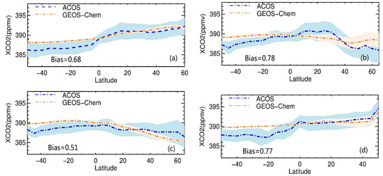
Figure 2.
XCO2 concentrations of GOSAT/ACOSv7.3 and GEOS-Chem averaged over 5° latitude bins during March 2010–February 2011: (a) MAM; (b) JJA; (c) SON; (d) DJF. Blue lines denote the latitudinal mean GOSAT/ACOSv7.3 XCO2 data, with the light blue envelope representing their standard deviation. Orange line and light orange envelope denotes the latitudinal mean GEOS-Chem XCO2 concentrations and their corresponding standard deviation.
The seasonal correlation coefficients of XCO2 between GOSAT/ACOS and GEOS-Chem in Figure 3 show that best correlation (R = 0.80) is found in MAM and the poorest correlation (R = 0.52) in SON. Cogan et al. [26] also found that GEOS-Chem (v08-02) showed highest correlation with GOSAT observation (UoL-FP retrievals) in MAM.
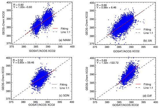
Figure 3.
Scatter plots of XCO2 retrievals of GOSAT/ACOS v7.3 versus XCO2 simulation from GEOS-Chem during March 2010–February 2011. (a)–(d) indicate MAM, JJA, SON and DJF respectively. Unit: ppm.
In addition, as shown in Figure 4, the time series variations of XCO2 from GEOS-Chem in the NH during April 2009–December 2011 show good agreement with those of GOSAT/ACOSv7.3, but monthly averaged XCO2 in the SH is obviously overestimated by GEOS-Chem (even up to 2.5 ppm in April 2011). Overall, the average bias between GEOS-Chem and GOSAT/ACOS is 0.78 ppm (GEOS-Chem −GOSAT/ACOS) on the global land during April 2009–December 2011. From Figure 4, in the NH, the CO2 seasonal cycle dependence of GOSAT/ACOSv7.3 is stronger than GEOS-Chem in JJA.
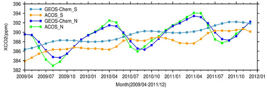
Figure 4.
The time series variations of monthly averaged XCO2 for April 2009–December 2011 in the NH and SH between GOSAT/ACOS and GEOS-Chem. The green line denote the GOSAT/ACOS XCO2 retrievals in the NH and the orange one is in the SH; the two blue lines refers to the XCO2 simulated from GEOS-Chem in the NH and SH respectively.
Monthly averaged XCO2 result in Table 2 and time series variations of the NH in Figure 4 also reveal the largest difference (1.2 ppm) between GEOS-Chem and GOSAT/ACOS found in JJA. This phenomenon coincides with the seasonal drawdown of XCO2 and therefore may be connected to the biospheric fluxes in the GEOS-Chem model. Li et al. [18] stated that the uncertainty in the terrestrial biosphere has a strong effect on CO2 simulations in summer.
Table 2.
Statistics of the number of XCO2 data (N), standard deviation (STD) and averaged biases (Bias) for GEOS-Chem (G-C), GOSAT/ACOS (G-A for GEOS-Chem −ACOS) over the global land during March 2010–February 2011. Unit: ppm.
Additionally, the result from Table 2 indicates that monthly averaged biases (GEOS-Chem—GOSAT/ACOS) during March 2010–December 2011 ranging from −0.11 ppm to 1.23 ppm. However, Lei et al. [19] found that the bias between GEOS-Chem and GOSAT (NIES algorithm) XCO2 could be up to around 3.3 ppm. This discrepancy between our study and Lei et al. [19] could be due to different retrieval algorithms of GOSAT and different version of GEOS-Chem model simulation.
From Table 2, the monthly averaged standard deviation of GOSAT/ACOSv7.3 XCO2 is relatively larger (even up to 3.5 ppm) than that of XCO2 simulated from GEOS-Chem, indicating the more discrete variation of GOSAT/ACOSv7.3 XCO2 than those of GEOS-Chem. This phenomenon is similar to the result shown in Figure 2. The reason for more discrete variations of GOSAT/ACOS XCO2 may be that, on the one hand, the GEOS-Chem model is not better to capture complicated dynamic variations of XCO2 than satellite observations [15]. On the other hand, the retrieval errors on satellite observations [23,26] could lead to large uncertainties in the GOSAT/ACOSv7.3 XCO2.
4.2. Comparison with CarbonTracker XCO2
Satellite XCO2 retrievals are useful in analyzing XCO2 variability and informing carbon cycle science. Nonetheless, their limited observations probably lead to uncertainties in further interpreting their scientific significance [65]. Unlike satellite XCO2 retrievals, model simulations (e.g., GEOS-Chem) can provide full-coverage maps of CO2 concentrations on the global or regional scale. To further compare the differences between GEOS-Chem and CarbonTracker, global CO2 profiles from GEOS-Chem, CT2013 and CT2016 are converted to XCO2 using Equation (2) in this section. In view of a high similarity of input surface fluxes in GEOS-Chem and CT2013B, we mainly analyze the spatial distribution, seasonal correlation and time series variations of XCO2 between GEOS-Chem and CT2013B.
The spatial distribution of XCO2 between GEOS-Chem and CT2013B in Figure 5 indicates that significant seasonal variations of global atmospheric CO2 are found from these two model simulations. The difference (GEOS-Chem −CT2013B) result shows that the seasonal averaged XCO2 of GEOS-Chem is slightly underestimated relative to that of CT2013B at most regions on the global scale, apart from eastern China and middle Africa in MAM, SON and DJF, northern South America as well as high latitude of the NH in JJA. Here, we simply analyze the overestimated effect in these regions. From Figure 6, limited assimilated observation sites for CT2013B are found in these regions, therefore, the assimilated effect of CT2013B is small and not discussed in these regions. From Table 1, GEOS-Chem used ODIAC as fossil fuel emission input, and CT2013B simultaneously used ODIAC and Miller dataset. CT2013B document [59] reported that large fossil emission differences between ODIAC and Miller datasets were found in eastern China, although ODIAC and Miller have similar global emissions for each year. Overestimated XCO2 from GEOS-Chem over eastern China may be due to the effect of fossil fuel emission inventory differences. For middle Africa and northern South America, overestimated XCO2 from GEOS-Chem is probably related to spatial distribution differences in terrestrial biosphere fluxes between GFED3 and GFED2. These spatial differences between GFED3 and GFED2 were also described by CT2013 document [59]. For more details, please see the CT2013 document [59]. For the high latitude region in the NH, the difference of biosphere fluxes and fossil fuel emission in this region used in GEOS-Chem and CT2013B is very small according to CT2013B document [59], but transport models are different. Therefore, overestimated XCO2 from GEOS-Chem in summer for the high latitudes of NH are likely affected by atmospheric transport and local fluxes.
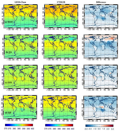
Figure 5.
Comparison of global XCO2 simulated with GEOS-Chem and CT2013B during March 2010–February 2011. Seasonal averaged XCO2 concentrations are shown for GEOS-Chem, CT2013B and their difference (GEOS-Chem −CT2013B). (a) MAM; (b) JJA; (c): SON; (d): DJF. Unit: ppm.
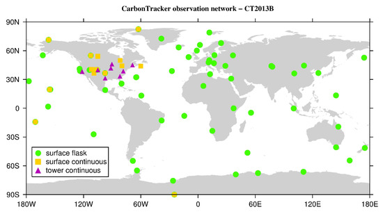
Figure 6.
The spatial distribution of CT2013B assimilated observational network (source: CarbonTracker website).
The seasonal correlation in Figure 7 shows that the highest correlation of XCO2 (up to 0.98) between GEOS-Chem and CT2013B is found in MAM, with an average bias of −0.59 ppm, while the poorest correlation also reached approximately 0.93 in SON, with the smallest average bias of −0.37 ppm. The XCO2 from these two models show very good correlation for each season on the whole, but remarkably overestimated XCO2 for GEOS-Chem (more than 6 ppm) are found in Figure 7b, which mainly located at high latitude of the NH as shown in Figure 5.
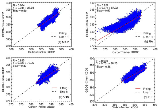
Figure 7.
Scatter plots of XCO2 from CarbonTracker (CT2013B) versus that of GEOS-Chem during March 2010–February 2011. (a)–(d) indicate MAM, JJA, SON and DJF respectively. Unit: ppm.
Figure 8 shows that there is good agreement among GEOS-Chem, CT2013B and CT2016 with regard to the seasonal cycle of monthly averaged XCO2 during 2009–2011. As presented in Table 1, both GEOS-Chem and CT2013B use CASA biospheric flux (GFED3 or GFED2) as their input surface flux. Lindqvist et al. [29] reported that biospheric flux is closely connected to seasonal cycle of CO2. Nearly identical time series variation of XCO2 in JJA and SON in Figure 8 between GEOS-Chem and CT2013B are probably influenced by similar biospheric flux components. This result was also reported by Lindqvist et al. [23]. However, CT2013B Document [59] have found that the newer CASA-GFEDv3 product has a smaller seasonal cycle than the older CASA-GFEDv2. Compared with the time series of CT2013B, the global XCO2 simulated from GEOS-Chem were slightly underestimated on the whole, which may be due to the newer CASA-GFEDv3 biospheric flux used in GEOS-Chem, as well as different transport models or the assimilation of observation data (e.g., GLOBALVIEW data) from CT2013B. Furthermore, the CT2013B show nearly identical variation with the CT2016 due to their similar input surface fluxes and transport models (shown in Table 1). However, due to the difference of biospheric flux version, their seasonal cycle shows a little discrepancies in JJA.
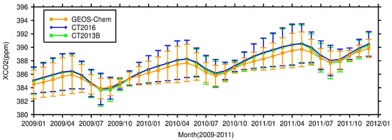
Figure 8.
The time series variations of monthly averaged XCO2 and standard deviation for 2009–2011 among CT2013B, CT2016 and GEOS-Chem on the global scale. The orange line is the XCO2 simulated from GEOS-Chem; the blue line refers to XCO2 simulated from CT2016; the green line is the XCO2 of CT2013B. Unit: ppmv.
For standard deviation, most of the monthly averaged XCO2 from CT2013B shows a slightly larger discrete variation than the GEOS-Chem model. The larger discrete variation in CT2013B may be due to different transport models, as well as the assimilation of observation data (e.g., GLOBALVIEW data) in the CT2013B.
4.3. Comparison with TCCON XCO2 Measurements
To further validate the GEOS-Chem CO2 simulations, ground-based TCCON measurements during 2009–2011 were used in this study. Since TCCON measurements were XCO2 observations, the model-simulated CO2 profiles need to be first sampled at the location of TCCON observation and integrated to XCO2 by using the TCCON averaging kernels and a priori profiles as described in Section 3. The ground-based XCO2 retrievals from fourteen TCCON sites were compared to the modeled CO2 from GEOS-Chem at around 13:00 ± 2 h local time.
The comparison result in Figure 9 shows that evident time series variations of XCO2 from the GEOS-Chem model and TCCON sites are observed in the NH sites, e.g., Bialystok, Lamont, Park Falls, Garmisch, and Orleans. No obviously seasonal variations were found in Wollongong, Darwin and Lauder sites of the SH. The XCO2 comparisons in Figure 10 and Table 3 reveal that the model bias at most sites is within ±1.0 ppm, except at Eureka (−1.2 ppm). The model bias is relatively smaller in the SH sites (<0.5 ppm) than those in the NH sites (<1.2 ppm). However, relative to GOSAT/ACOS, the model bias is a litter larger in the SH than that in the NH. The result in Figure 10a and Table 3 also indicates that modeled XCO2 from GEOS-Chem are underestimated at most sites, which shows good agreement with the result from comparison with CT2013B. Other studies also reported the underestimated effect of XCO2 in model simulation (e.g., ACTM, TM5 models) [20,66]. However, overestimated XCO2 from GEOS-Chem are found at some sites, including Garmisch (+0.79 ppm), Karlsruhe (+0.03 ppm), Sodankylä (+0.68 ppm) and Ny-Ålesund(+0.37 ppm). As for Garmisch, complex geographical terrain (valleys) at station probably result in model overestimation. For Sodankylä and Ny-Ålesund sites in the far north, model overestimation of CO2 is likely caused by atmospheric transport and local fluxes that has been discussed in Section 4.2. This result is also similar to the performance of the NIES TM model, which shows a larger bias (+1.22 ppm) for XCO2 over Sodankylä [67].
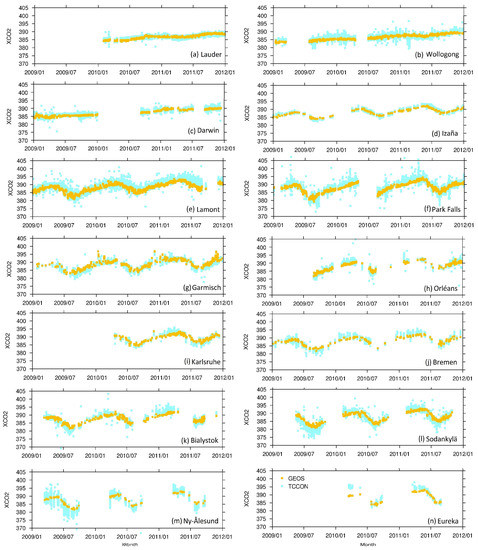
Figure 9.
Comparison of XCO2 from GEOS-Chem (yellow dots) and ground-based TCCON XCO2 measurements (blue dots) during 2009–2011: (a) Lauder; (b) Wollongong; (c) Darwin; (d) Izaña; (e) Lamont; (f) Park Falls; (g) Garmisch; (h) Orleans; (i) Karlsruhe; (j) Bremen; (k) Bialystok; (l) Sodankylä; (m) Ny-Ålesund; (n) Eureka.
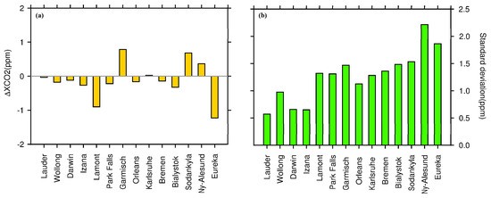
Figure 10.
Bias and root-mean-square error (RMSE) of GEOS-Chem model vs. TCCON sites in 2010. (a) model bias; (b) RMSE. Unit: ppm.
Table 3.
Statistics of number of XCO2 data (N) at TCCON sites, averaged XCO2, correlation coefficient (R), averaged bias (Bias) and root-mean-square error (RMSE) between GEOS-Chem (G-C) and TCCON during 2009–2011.
As presented in Table 3, XCO2 from GEOS-Chem show strong correlation with the TCCON data (R > 0.83), indicating a good representation of transport and fluxes in GEOS-Chem for simulated CO2. However, in the far north (Eureka and Sodankylä, Finland), the result show good correlation (R > 0.9) but the model bias is relatively high (>0.5 ppm), which is probably caused by atmospheric transport and local flux in high latitude of the NH. From Figure 10b and Table 3, the root-mean-square error (RMSE) also show small differences between GEOS-Chem and TCCON sites, with the largest RMSE (2.21 ppm) at the Ny-Ålesund site located in the far north. The RMSE is somewhat smaller at the SH stations than most of the NH sites, except Izaña site.
Seasonal biases can affect the seasonal cycle amplitude, and the seasonal cycle is important for biospheric flux attribution [68]. From Figure 11, in MAM and DJF, the modeled XCO2 from GEOS-Chem are underestimated at most sites, except Garmisch and Izaña. However, similar to Figure 10 and Table 3, the overestimated XCO2 occurred at the sites of high latitude of the NH in JJA, especially overestimated seasonal bias more than 1 ppm found at Sodankylä and Ny-Ålesund sites. This comparison result is also consistent with that of GOSAT/ACOS as well as CT2013B and probably related to transport model and local flux in GEOS-Chem.
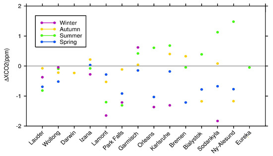
Figure 11.
Variations of seasonal biases between GEOS-Chem and TCCON sites during March 2010–December 2011: MAM, blue; JJA, green; SON; yellow and DJF, purple.
The seasonal cycle of XCO2 is closely related to the biospheric fluxes that determine the global terrestrial net CO2 sinks [23]. To compare the seasonal cycle of XCO2 from GEOS-Chem and TCCON sites, we use the NOAA fitting software CCGCRV [69] to statistically fit the seasonal cycle and yearly growth of XCO2. Constrained by short time series or large data gaps, only seven sites in the NH are used to extract the seasonal cycle of XCO2 in this study. It is noted that the detrended seasonal cycle is calculated by removing the long-term trends of XCO2. From Figure 12, the seasonal cycles in GEOS-Chem XCO2 are in good agreement with those of TCCON sites, for example, no apparent mismatches found at the Garmisch, Park Falls and Lamont sites. However, seasonal cycle amplitudes of XCO2 are obviously underestimated by GEOS-Chem at some sites, such as Bialystok, Bremen and Sodankylä sites, which may be due to the biospheric fluxes or transport in model. The result also shows consistency with previous studies, reporting an underestimation of XCO2 peak-to trough amplitudes in models [23,66]. From Table 4, the average yearly growth rate varies from 1.90 ppm year−1 to 2.37 ppm year−1 for GEOS-Chem and TCCON measurements during 2009–2011. The GEOS-Chem model shows a lower XCO2 growth rate than those of TCCON sites.
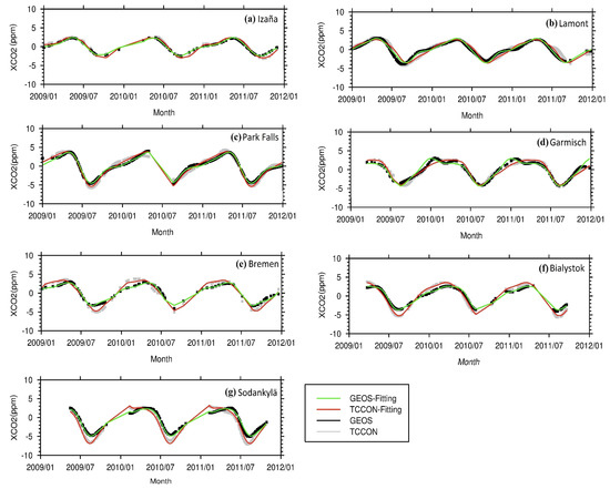
Figure 12.
Seasonal cycles of XCO2 are compared for GEOS-Chem and TCCON in the Northern Hemisphere during 2009–2011, which is calculated by removing the long-term trends of XCO2 (gray dots for TCCON, black dots for GEOS-Chem); smoothed lines is fitting seasonal cycle (red for TCCON, green for GEOS-Chem).
Table 4.
Comparison of the seasonal cycle amplitude and yearly growth rate between XCO2 of GEOS-Chem and TCCON sites. Sites included Izaña, Lamont, Park Falls, Garmisch, Bremen, Bialystok, and Sodankylä.
We also investigate mean bias, RMSE and correlation coefficients between TCCON sites and GEOS-Chem as well as GOSAT/ACOS during April 2009–December 2011. Considering of CO2 data availability at TCCON sites, only 9 TCCON sites including Bialystok, Bremen, Darwin, Garmisch, Lauder, Lamont, Orleans, Park Falls and Wollongong are used in this section. Similar to Cogan et al. [26], the averaging kernel and a priori have not been adopted in comparison between GOSAT/ACOS and TCCON sites, but they are used when comparing modeled CO2 from GEOS-Chem with TCCON sites.
As shown by Figure 13, the overall correlations between XCO2 from GEOS-Chem as well as GOSAT/ACOS and 9 TCCON sites are 0.93 and 0.74 respectively. The mean biases of XCO2 is −0.06 ppm between GEOS-Chem and TCCON sites, and −0.2 ppm between GOSAT/ACOS and TCCON sites, and their RMSE is 1.19 ppm and 2.05 ppm respectively. The result show that the modeled XCO2 from GEOS-Chem is underestimated on the whole by comparison with TCCON sites. Also, the result also indicate that XCO2 retrievals from GOSAT/ACOSv7.3 show somewhat underestimated effect by comparison with TCCON sites, which may be due to retrieval errors or instrument issue of the GOSAT [23,26,68]. These results show good consistency with Section 4 and Cogan et al. [26].
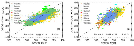
Figure 13.
The scatter plot of XCO2 between GEOS-Chem as well as GOSAT/ACOS and 9 TCCON sites during April 2009–December 2011. (a) The scatter plot between XCO2 from GEOS-Chem and XCO2 from TCCON sites; (b) The scatter plot between XCO2 from GOSAT/ACOS and XCO2 from TCCON sites.
5. Discussion
In this study, the comparison method mainly considered the averaging kernels among different CO2 data according to Wunch et al. [28]. While horizontal CO2 variability and differences in spatial support should be also considered in the future due to their impact in inter-comparison between different remote sensing observations [70]. For example, TCCON provide XCO2 observations at a point location, and GOSAT/ACOS observation represents an average XCO2 within the footprint 10.5 km in diameter [70]. The differences in spatial support may introduce another uncertainties when directly comparing between model results and observations [70]. Tadić and Michalak reported that different spatial support can lead to differences exceeding 0.5 ppm even for co-located CO2 observations [70]. To roughly estimate the uncertainty raised from the spatial support, we compared the differences between the XCO2 of GOSAT/ACOS (or TCCON sites) and the spatially averaged XCO2 of GOSAT/ACOS (or TCCON sites) in a 2° × 2.5° grid which is in line with the horizontal resolution of GEOS-Chem CO2 results.
From Figure 14, the differences (standard deviation) between GOSAT/ACOS XCO2 observations and the corresponding averaged XCO2 (at a 2° × 2.5° grid) ranged from 0–0.3 ppm and mostly distributed at 0–0.05 ppm. To some extent, these differences can be deemed as the impact of spatial support. To further understand the impact of averaged XCO2 at 2° × 2.5° grids, we recalculated the correlation, averaged bias and RMSE between GOSAT/ACOS and GEOS-Chem at GOSAT footprint scale (using averaging kernels but no spatial support was considered) and 2° × 2.5° scales (using averaging kernels and then calculating the average), respectively, using data of 2010 on the global land. Table 5 shows that the correlation (R) is less affected by the effect of spatial support, while the mean bias and RMSE can be impacted by different spatial support.
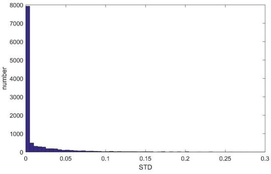
Figure 14.
The frequency histogram of differences (standard deviations) between GOSAT XCO2 and the corresponding averaged XCO2 at 2° × 2.5° grids on the global land in 2010.
Table 5.
Comparison between XCO2 from GEOS-Chem and GOSAT/ACOS in 2010. It is noted that comparison of averaged XCO2 between GEOS-Chem and GOSAT/ACOS observations at 2° × 2.5° grids was conducted after using averaging kernels.
Similarly, 14 TCCON sites were also used to estimate the uncertainties of the spatial support and they include Lamont, Park Falls, Bialystok, Orleans, Garmisch, Bremen, Sodankylä, Ny-Ålesund, Izaña, Eureka, Karlsruhe, Wollongong, Darwin, Lauder. From Figure 15, the differences (standard deviation) between XCO2 at 14 TCCON sites and averaged XCO2 at 2° × 2.5° grids mainly ranged from 0–1.4 ppm and mostly distributed at 0–0.1 ppm. This result indicates that different spatial support may bring relatively large uncertainties when directly comparing TCCON sites and GEOS-Chem.
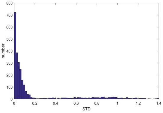
Figure 15.
The frequency histogram of differences (standard deviations) between TCCON XCO2 (14 sites) and the corresponding averaged XCO2 in 2010 at 2° × 2.5° grids.
Also, the correlation, averaged bias and RMSE between XCO2 from TCCON sites and GEOS-Chem in 2010 (Figure 16 and Table 6) were also calculated, which is similar to that of GOSAT/ACOS and GEOS-Chem. Similar to the comparison between GEOS-Chem and GOSAT, from Figure 16 and Table 6, we can see that the correlation is not affected by the spatial support, while the bias and RMSE is slightly affected.
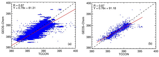
Figure 16.
The scatter plots between XCO2 from TCCON sites and GEOS-Chem ((a) using averaging kernels without considering the spatial support; (b) using averaging kernels and then calculating the average) in 2010.
Table 6.
Comparison between XCO2 from GEOS-Chem and TCCON sites in 2010.
By comparing Figure 14 and Figure 15, it is revealed that the impact of spatial support is more obvious for TCCON sites than that of GOSAT/ACOS measurements when comparing with GEOS-Chem results. This may be due to the spatial support of GOSAT/ACOS is more close to that of GEOS-Chem than TCCON. Furthermore, the correlation analysis between GEOS-Chem and TCCON sites (or GOSAT/ACOS) indicates that the spatial support has no obvious effect on the correlation coefficient. However, the mean bias and RMSE is indeed influenced by spatial support. Therefore, the uncertainties from spatial support should be pay enough attention in the future, especially for comparison with TCCON XCO2 point observations.
6. Conclusions
Global atmospheric CO2 concentrations were effectively simulated by a global 3-D chemical transport model (GEOS-Chem) during the years of 2009–2011 and compared with XCO2 data from the GOSAT satellite, CarbonTracker CO2 modeling system and TCCON measurements in this study. The results indicate that the modeled XCO2 from GEOS-Chem shows overall good consistency with GOSAT/ACOSv7.3, CarbonTracker, but the GEOS-Chem model overestimates XCO2 values compared with the GOSAT/ACOSv7.3 XCO2 retrievals at most regions, particularly in the SH and the high latitude of the NH.
The results also show that the monthly averaged XCO2 of GEOS-Chem generally underestimate XCO2 as compared to CarbonTracker, although they have a similar seasonal cycle. The discrepancies between the two models may be originated from a different transport model or the assimilation of observation in CarbonTracker. However, obvious overestimated XCO2 from GEOS-Chem was found at the high latitudes of the Northern Hemisphere in JJA as compared with CarbonTracker or TCCON sites, which indicates that large uncertainties in GEOS-Chem over these regions probably because of the influences of atmospheric transport model and local flux. This phenomenon has been also reflected by comparison with GOSAT/ACOS.
Overall, although the simulated CO2 from GEOS-Chem are in a good agreement with the GOSAT/ACOS retrievals, CarbonTracker and TCCON measurements, the discrepancies between them are considerable, e.g., the underestimation effect of XCO2 in GEOS-Chem model, probably due to lack of constraints from measurements and affected by prior biosphere flux in model. Also, the obvious overestimated XCO2 in the high latitude of the NH in JJA is needed to be concerned. Future work will need to assimilate observation data, e.g., GOSAT/ACOS or OCO-2, into the GEOS-Chem model to further optimize the CO2 fluxes. These comparisons and analysis also indicated that GOSAT/ACOSv7.3 retrievals could underestimate the XCO2. The uncertainties in satellite observations are necessary to quantify for further estimations of their assimilation into model systems. Furthermore, the uncertainties from spatial support should be carefully considered when inter-comparison among different observations and models.
Author Contributions
The work presented in this paper was carried out in a collaboration between all authors. The study was conceived by Y.J., T.W., P.Z., L.C., N.X. and Y.M. The writing was led by Y.J., T.W., P.Z., L.C., N.X. and Y.M. All authors contributed to reviewing and revising the text.
Acknowledgments
This work was supported by the National Natural Science Foundation of China (Grant No. 41475031, No. 41471304, No. 41571364 and No. 41771387) and China Postdoctoral Science Foundation (Grant No. 2016M590074).We acknowledge the ACOS/OCO-2 project at the Jet Propulsion Laboratory, California Institute of Technology and NASA Goddard Earth Science Data and Information Services Center for providing the ACOS7.3 XCO2 data archive. CarbonTracker CT2013B results provided by NOAA ESRL, Boulder, Colorado, USA from the website at http://carbontracker.noaa.gov. In addition, TCCON data were obtained from the TCCON Data Archive, hosted by the Carbon Dioxide Information Analysis Center (CDIAC)—tccondata.org. We also thank David Griffith for his suggestion about the use of TCCON averaging kernels in comparison with GEOS-Chem model. We are also grateful for the GEOS-Chem model managed by the GEOS-Chem Support Team Support Team, based at Harvard University and Dalhousie University. Finally, we thanks for all reviewers for their comments about this manuscript, especially his/her suggestion about the uncertainties from spatial support.
Conflicts of Interest
The authors declare no conflict of interest.
References
- Intergovernmental Panel on Climate Change (IPCC). Summary for policymakers. In Climate Change: The Physical Science Basis; Contribution of Working Group I to the Fifth Assessment Report of the Intergovernmental Panel on Climate Change; Cambridge University Press: Cambridge, UK; New York, NY, USA, 2013. [Google Scholar]
- Solomon, S.; Intergovernmental Panel on Climate Change; Intergovernmental Panel on Climate Change, Working Group I. Climate Change 2007: The Physical Science Basis: Contribution of Working Group I to the Fourth Assessment Report of the Intergovernmental Panel on Climate Chang; Cambridge University Press: Cambridge, UK; New York, NY, USA, 2007. [Google Scholar]
- Shakun, J.D.; Clark, P.U.; He, F.; Marcott, S.A.; Mix, A.C.; Liu, Z.; Otto-Bliesner, B.; Schmittner, A.; Bard, E. Global warming preceded by increasing carbon dioxide concentrations during the last deglaciation. Nature 2012, 484, 49–54. [Google Scholar] [CrossRef] [PubMed]
- Friedlingstein, P.; Cox, P.; Betts, R.; Bopp, L.; von Bloh, W.; Brovkin, V.; Cadule, P.; Doney, S.; Eby, M.; Fung, I.; et al. Climate-carbon cycle feedback analysis: Results from the C4MIP model intercomparison. J. Clim. 2006, 19, 3337–3353. [Google Scholar] [CrossRef]
- Butz, A.; Hasekamp, O.P.; Frankenberg, C.; Aben, I. Retrievals of atmospheric CO2 from simulated space-borne measurements of backscattered near-infrared sunlight: Accounting for aerosol effects. Appl. Opt. 2009, 48, 3322–3336. [Google Scholar] [CrossRef] [PubMed]
- O’Dell, C.W.; Connor, B.; Bösch, H.; O’Brien, D.; Frankenberg, C.; Castano, R.; Christi, M.; Eldering, D.; Fisher, B.; Gunson, M.; et al. The ACOS CO2 retrieval algorithm—Part 1: Description and validation against synthetic observations. Atmos. Meas. Tech. 2012, 5, 99–121. [Google Scholar] [CrossRef]
- Reuter, M.; Buchwitz, M.; Schneising, O.; Heymann, J.; Bovensmann, H.; Burrows, J.P. A method for improved SCIAMACHY CO2 retrieval in the presence of optically thin clouds. Atmos. Meas. Tech. 2010, 3, 209–232. [Google Scholar] [CrossRef]
- Yokota, T.; Yoshida, Y.; Eguchi, N.; Ota, Y.; Tanaka, T.; Watanabe, H.; Maksyutov, S. Global Concentrations of CO2 and CH4 Retrieved from GOSAT: First Preliminary Results. Sola 2009, 5, 160–163. [Google Scholar] [CrossRef]
- Frankenberg, C.; Pollock, R.; Lee, R.A.M.; Rosenberg, R.; Blavier, J.F.; Crisp, D.; O’Dell, C.W.; Osterman, G.B.; Roehl, C.; Wennberg, P.O.; et al. The Orbiting Carbon Observatory (OCO-2): Spectrometer performance evaluation using pre-launch direct sun measurements. Atmos. Meas. Tech. 2015, 8, 301–313. [Google Scholar] [CrossRef]
- Chen, X.; Wang, J.; Liu, Y.; Xu, X.; Cai, Z.; Yang, D.; Yan, Y.; Feng, L. Angular dependence of aerosol information content in CAPI/TanSat observation over land: Effect of polarization and synergy with A-Train satellites. Remote Sens. Environ. 2017, 196, 163–177. [Google Scholar] [CrossRef]
- Crisp, D.; Fisher, B.; O’Dell, C.; Frankenberg, C.; Basilio, R.; Bosch, H.; Brown, L.R.; Castano, R.; Connor, B.; Deutscher, N.M.; et al. The ACOS CO2 retrieval algorithm—Part II: Global XCO2 data characterization. Atmos. Meas. Tech. 2012, 5, 687–707. [Google Scholar] [CrossRef]
- Wang, T.X.; Shi, J.C.; Jing, Y.Y.; Xie, Y.H. Investigation of the consistency of atmospheric CO2 retrievals from different space-based sensors: Intercomparison and spatiotemporal analysis. Chin. Sci. Bull. 2013, 58, 4161–4170. [Google Scholar] [CrossRef]
- Jing, Y.; Shi, J.; Wang, T.; Sussmann, R. Mapping Global Atmospheric CO2 Concentration at High Spatiotemporal Resolution. Atmosphere 2014, 5, 870–888. [Google Scholar] [CrossRef]
- Griffith, D.W.; Toon, G.C.; Connor, B.; Sussmann, R.; Warneke, T.; Deutscher, N.M.; Wennberg, P.O.; Notholt, J.; Sherlock, V.; Robinson, J.; et al. Preliminary validation of column-averaged volume mixing ratios of carbon dioxide and methane retrieved from GOSAT short-wavelength infrared spectra. Atmos. Meas. Tech. 2011, 4, 1061–1076. [Google Scholar] [CrossRef]
- Zhang, H.; Chen, B.; Xu, G.; Yan, J.; Che, M.; Chen, J.; Fang, S.; Lin, X.; Sun, S. Comparing simulated atmospheric carbon dioxide concentration with GOSAT retrievals. Chin. Sci. Bull. 2015, 60, 380–386. [Google Scholar] [CrossRef]
- Gurney, K.R.; Law, R.M.; Denning, A.S.; Rayner, P.J.; Baker, D.; Bousquet, P.; Bruhwiler, L.; Chen, Y.H.; Ciais, P.; Fan, S.; et al. TransCom 3 CO2 inversion intercomparison: 1. Annual mean control results and sensitivity to transport and prior flux information. Tellus B 2003, 55, 555–579. [Google Scholar] [CrossRef]
- Chevallier, F.; Feng, L.; Bösch, H.; Palmer, P.I.; Rayner, P.J. On the impact of transport model errors for the estimation of CO2 surface fluxes from GOSAT observations. Geophys. Res. Lett. 2010, 37. [Google Scholar] [CrossRef]
- Li, R.; Zhang, M.; Chen, L.; Kou, X.; Skorokhod, A. CMAQ simulation of atmospheric CO2 concentration in East Asia: Comparison with GOSAT observations and ground measurements. Atmos. Environ. 2017, 160, 176–185. [Google Scholar] [CrossRef]
- Lei, L.; Guan, X.; Zeng, Z.; Zhang, B.; Ru, F.; Bu, R. A comparison of atmospheric CO2 concentration GOSAT-based observations and model simulations. Sci. China Earth Sci. 2014, 57, 1393–1402. [Google Scholar] [CrossRef]
- Saito, R.; Patra, P.K.; Deutscher, N.; Wunch, D.; Ishijima, K.; Sherlock, V.; Blumenstock, T.; Dohe, S.; Griffith, D.; Hase, F.; et al. Latitude-time variations of atmospheric column-average dry air mole fractions of CO2, CH4 and N2O. Atmos. Chem. Phys. 2012, 12, 7767–7777. [Google Scholar] [CrossRef]
- Nassar, R.; Jones, D.B.; Suntharalingam, P.; Chen, J.M.; Andres, R.J.; Wecht, K.; Yantosca, R.M.; Kulawik, S.S.; Bowman, K.W.; Worden, J.R.; et al. Modeling Global Atmospheric CO2 with Improved Emission Inventories and CO2 Production from the Oxidation of Other Carbon Species. Geosci. Model Dev. 2010, 3, 689–716. [Google Scholar] [CrossRef]
- Feng, L.; Palmer, P.I.; Yang, Y.; Yantosca, R.M.; Kawa, S.R.; Paris, J.D.; Matsueda, H.; Machida, T. Evaluating a 3-D transport model of atmospheric CO2 using ground-based, aircraft, and space-borne data. Atmos. Chem. Phys. 2011, 11, 2789–2803. [Google Scholar] [CrossRef]
- Lindqvist, H.; O’Dell, C.W.; Basu, S.; Boesch, H.; Chevallier, F.; Deutscher, N.; Feng, L.; Fisher, B.; Hase, F.; Inoue, M.; et al. Does GOSAT capture the true seasonal cycle of carbon dioxide. Atmos. Chem. Phys. 2015, 15, 13023–13040. [Google Scholar] [CrossRef]
- Zhang, L.L.; Yue, T.X.; Wilson, J.P.; Zhao, N.; Zhao, Y.P.; Du, Z.P.; Liu, Y. A comparison of satellite observations with the XCO2 surface obtained by fusing TCCON measurements and GEOS-Chem model outputs. Sci. Total Environ. 2017, 601, 1575–1590. [Google Scholar] [CrossRef] [PubMed]
- Yoshida, Y.; Ota, Y.; Eguchi, N.; Kikuchi, N.; Nobuta, K.; Tran, H.; Morino, I.; Yokota, T. Retrieval algorithm for CO2 and CH4 column abundances from short-wavelength infrared spectral observations by the Greenhouse gases observing satellite. Atmos. Meas. Tech. 2011, 4, 717–734. [Google Scholar] [CrossRef]
- Cogan, A.J.; Boesch, H.; Parker, R.J.; Feng, L.; Palmer, P.I.; Blavier, J.F.; Deutscher, N.M.; Macatangay, R.; Notholt, J.; Roehl, C.; et al. Atmospheric carbon dioxide retrieved from the Greenhouse gases Observing SATellite (GOSAT): Comparison with ground-based TCCON observations and GEOS-Chem model calculations. J. Geophys. Res. Atmos. 2012, 117. [Google Scholar] [CrossRef]
- Osterman, G.; Eldering, A.; Cheng, C.; O’Dell, C.; Martinez, E.; Crisp, D.; Frankenberg, C.; Fisher, B.; Wunch, D. ACOS Level 2 Standard Product and Lite Data Product Data User’s Guide, v7.3; GES DISC: Greenbelt, MD, USA, 2017. [Google Scholar]
- Wunch, D.; Toon, G.C. Calibration of the Total Carbon column Observing Network using aircraft profile data. Atmos. Meas. Tech. 2010, 3, 1351–1362. [Google Scholar] [CrossRef]
- Wunch, D.; Toon, G.C.; Blavier, J.-F.L.; Washenfelder, R.A.; Notholt, J.; Connor, B.J.; Griffith, D.W.T.; Sherlock, V.; Wennberg, P.O. The Total Carbon Column Observing Network. Philos. Trans. R. Soc. A Math. Phys. Eng. Sci. 2011, 369, 2087–2112. [Google Scholar] [CrossRef] [PubMed]
- Messerschmidt, J.; Geibel, M.C.; Blumenstock, T.; Chen, H.; Deutscher, N.M.; Engel, A.; Feist, D.G.; Gerbig, C.; Gisi, M.; Hase, F.; et al. Calibration of TCCON column-averaged CO2: The first aircraft campaign over European TCCON sites. Atmos. Chem. Phys. 2011, 11, 10765–10777. [Google Scholar] [CrossRef]
- Wennberg, P.O.; Wunch, D.; Roehl, C.; Blavier, J.-F.; Toon, G.C.; Allen, N.; Dowell, P.; Teske, K.; Martin, C.; Martin, J. TCCON Data from Lamont, Oklahoma, USA, Release GGG2014.R1. TCCON Data Archive, Hosted by the Carbon Dioxide Information Analysis Center, Oak Ridge National Laboratory, Oak Ridge, Tennessee, U.S.A.; Oak Ridge National Laboratory: Oak Ridge, TN, USA, 2016. [CrossRef]
- Wennberg, P.O.; Roehl, C.; Wunch, D.; Toon, G.C.; Blavier, J.-F.; Washenfelder, R.; Keppel-Aleks, G.; Allen, N.; Ayers, J. TCCON Data from Park Falls, Wisconsin, USA, Release GGG2014R0. TCCON Data Archive, Hosted by the Carbon Dioxide Information Analysis Center, Oak Ridge National Laboratory, Oak Ridge, Tennessee, U.S.A.; Oak Ridge National Laboratory: Oak Ridge, TN, USA, 2014. [CrossRef]
- Washenfelder, R.A.; Toon, G.C.; Blavier, J.F.; Yang, Z.; Allen, N.T.; Wennberg, P.O.; Vay, S.A.; Matross, D.M.; Daube, B.C. Carbon dioxide column abundances at the Wisconsin Tall Tower site. J. Geophys. Res. Atmos. 2006, 111, D22305. [Google Scholar] [CrossRef]
- Deutscher, N.; Notholt, J.; Messerschmidt, J.; Weinzierl, C.; Warneke, T.; Petri, C.; Grupe, P.; Katrynski, K. TCCON Data from Bialystok, Poland, Release GGG2014R1. TCCON Data Archive, Hosted by the Carbon Dioxide Information Analysis Center, Oak Ridge National Laboratory, Oak Ridge, Tennessee, U.S.A.; Oak Ridge National Laboratory: Oak Ridge, TN, USA, 2015. [CrossRef]
- Messerschmidt, J.; Chen, H.; Deutscher, N.M.; Gerbig, C.; Grupe, P.; Katrynski, K.; Koch, F.T.; Lavrič, J.V.; Notholt, J.; Rödenbeck, C.; et al. Automated ground-based remote sensing measurements of greenhouse gases at the Białystok site in comparison with collocated in situ measurements and model data. Atmos. Chem. Phys. 2012, 12, 6741–6755. [Google Scholar] [CrossRef]
- Warneke, T.; Messerschmidt, J.; Notholt, J.; Weinzierl, C.; Deutscher, N.; Petri, C.; Grupe, P.; Vuillemin, C.; Truong, F.; Schmidt, M.; et al. TCCON Data from Orleans, France, Release GGG2014R0. TCCON Data Archive, Hosted by the Carbon Dioxide Information Analysis Center, Oak Ridge National Laboratory, Oak Ridge, Tennessee, U.S.A.; Oak Ridge National Laboratory: Oak Ridge, TN, USA, 2014. [CrossRef]
- Messerschmidt, J.; Macatangay, R.; Notholt, J.; Petri, C.; Warneke, T.; Weinzierl, C. Side by side measurements of CO2 by ground-based Fourier transform spectrometry (FTS). Tellus B 2010, 62, 749–758. [Google Scholar] [CrossRef]
- Sussmann, R.; Rettinger, M. TCCON Data from Garmisch, Germany, Release GGG2014R0.TCCON Data Archive, Hosted by the Carbon Dioxide Information Analysis Center, Oak Ridge National Laboratory, Oak Ridge, Tennessee, U.S.A.; Oak Ridge National Laboratory: Oak Ridge, TN, USA, 2014. [CrossRef]
- Hausmann, P.; Sussmann, R.; Smale, D. Contribution of oil and natural gas production to renewed increase in atmospheric methane (2007–2014): Top–down estimate from ethane and methane column observations. Atmos. Chem. Phys. 2016, 16, 3227–3244. [Google Scholar] [CrossRef]
- Notholt, J.; Petri, C.; Warneke, T.; Deutscher, N.; Buschmann, M.; Weinzierl, C.; Macatangay, R.; Grupe, P. TCCON Data from Bremen, Germany, Release GGG2014R0. TCCON Data Archive, Hosted by the Carbon Dioxide Information Analysis Center, Oak Ridge National Laboratory, Oak Ridge, Tennessee, U.S.A.; Oak Ridge National Laboratory: Oak Ridge, TN, USA, 2014. [CrossRef]
- Kivi, R.; Heikkinen, P.; Kyro, E. TCCON Data from Sodankyla, Finland, Release GGG2014R0. TCCON Data Archive, Hosted by the Carbon Dioxide Information Analysis Center, Oak Ridge National Laboratory, Oak Ridge, Tennessee, U.S.A.; Oak Ridge National Laboratory: Oak Ridge, TN, USA, 2014. [CrossRef]
- Kivi, R.; Heikkinen, P. Fourier transform spectrometer measurements of column CO2 at Sodankylä, Finland. Geosci. Instrum. Methods Data Syst. 2016, 5, 271–279. [Google Scholar] [CrossRef]
- Blumenstock, T.; Hase, F.; Schneider, M.; Garcia, O.E.; Sepulveda, E. TCCON Data from Izana, Tenerife, Spain, Release GGG2014R0. TCCON Data Archive, Hosted by the Carbon Dioxide Information Analysis Center, Oak Ridge National Laboratory, Oak Ridge, Tennessee, U.S.A.; Oak Ridge National Laboratory: Oak Ridge, TN, USA, 2014. [Google Scholar] [CrossRef]
- Strong, K.; Mendonca, J.; Weaver, D.; Fogal, P.; Drummond, J.R.; Batchelor, R.; Lindenmaier, R. TCCON Data from Eureka, Canada, Release GGG2014R0. TCCON Data Archive, Hosted by the Carbon Dioxide Information Analysis Center, Oak Ridge National Laboratory, Oak Ridge, Tennessee, U.S.A.; Oak Ridge National Laboratory: Oak Ridge, TN, USA, 2016. [CrossRef]
- Hase, F.; Blumenstock, T.; Dohe, S.; Gross, J.; Kiel, M. TCCON Data from Karlsruhe, Germany, Release GGG2014R1. TCCON Data Archive, Hosted by the Carbon Dioxide Information Analysis Center, Oak Ridge National Laboratory, Oak Ridge, Tennessee, U.S.A.; Oak Ridge National Laboratory: Oak Ridge, TN, USA, 2015. [CrossRef]
- Griffith, D.W.T.; Velazco, V.A.; Deutscher, N.; Murphy, C.; Jones, N.; Wilson, S.; Macatangay, R.; Kettlewell, G.; Buchholz, R.R.; Riggenbach, M. TCCON Data from Wollongong, Australia, Release GGG2014R0. TCCON Data Archive, Hosted by the Carbon Dioxide Information Analysis Center, Oak Ridge National Laboratory, Oak Ridge, Tennessee, U.S.A.; Oak Ridge National Laboratory: Oak Ridge, TN, USA, 2014. [CrossRef]
- Griffith, D.W.T.; Deutscher, N.; Velazco, V.A.; Wennberg, P.O.; Yavin, Y.; Aleks, G.; Washenfelder, R.; Toon, G.C.; Blavier, J.-F.; Murphy, C.; et al. TCCON Data from Darwin, Australia, Release GGG2014R0. TCCON Data Archive, Hosted by the Carbon Dioxide Information Analysis Center, Oak Ridge National Laboratory, Oak Ridge, Tennessee, U.S.A.; Oak Ridge National Laboratory: Oak Ridge, TN, USA, 2014. [CrossRef]
- Deutscher, N.; Griffith, D.; Bryant, G.; Wennberg, P.; Toon, G.; Washenfelder, R.; Keppel-Aleks, G.; Wunch, D.; Yavin, Y.; Allen, N.; et al. Total column CO2 measurements at Darwin, Australia-site description and calibration against in situ aircraft profiles. Atmos. Meas. Tech. 2010, 3, 947–958. [Google Scholar] [CrossRef]
- Sherlock, V.; Connor, B.; Robinson, J.; Shiona, H.; Smale, D.; Pollard, D. TCCON Data Archive, Hosted by the Carbon Dioxide Information Analysis Center, Oak Ridge National Laboratory, Oak Ridge, Tennessee, U.S.A.; Oak Ridge National Laboratory: Oak Ridge, TN, USA, 2014. [CrossRef]
- Bey, I.; Jacob, D.J.; Yantosca, R.M.; Logan, J.A.; Field, B.D.; Fiore, A.M.; Li, Q.; Liu, H.Y.; Mickley, L.J.; et al. Global modeling of tropospheric chemistry with assimilated meteorology: Model description and evaluation. J. Geophys. Res. Atmos. 2001, 106, 23073–23095. [Google Scholar] [CrossRef]
- Suntharalingam, P.; Jacob, D.J.; Palmer, P.I.; Logan, J.A.; Yantosca, R.M.; Xiao, Y.; Evans, M.J.; Streets, D.; Vay, S.A.; Sachse, G. Improved quantification of Chinese carbon fluxes using CO2/CO correlations in Asian outflow. J. Geophys. Res. 2004, 109. [Google Scholar] [CrossRef]
- Andres, R.J.; Gregg, J.S.; Losey, L.; Marland, G.; Boden, T.A. Monthly, global emissions of carbon dioxide from fossil fuel consumption. Tellus B 2011, 63, 309–327. [Google Scholar] [CrossRef]
- Van der Werf, G.R.; Randerson, J.T.; Giglio, L.; Collatz, G.J.; Mu, M.; Kasibhatala, P.S.; Morton, D.C.; DeFries, R.S.; Jin, Y.; van Leeuwen, T.T. Global fire emissions and the contribution of deforestation, savanna, forest, agricultural, and peat fires (1997–2009). Atmos. Chem. Phys. 2010, 10, 11707–11735. [Google Scholar] [CrossRef]
- Olsen, S.C.; Randerson, J.T. Differences between surface and column atmospheric CO2 and implications for carbon cycle research. J. Geophys. Res. Atmos. 2004, 109. [Google Scholar] [CrossRef]
- Baker, D.F.; Law, R.M.; Gurney, K.R.; Rayner, P.; Peylin, P.; Denning, A.S.; Bousquet, P.; Bruhwiler, L.; Chen, Y.H.; Ciais, P.; et al. TransCom 3 inversion intercomparison: Impact of transport model errors on the interannual variability of regional CO2 fluxes, 1988–2003. Glob. Biogeochem. Cycles 2006, 20. [Google Scholar] [CrossRef]
- Takahashi, T.; Sutherland, S.C.; Wanninkhof, R.; Sweeney, C.; Feely, R.A.; Chipman, D.W.; Hales, B.; Friederich, G.; Chavez, F.; Sabine, C.; et al. Climatological mean and decadal change in surface ocean pCO2, and net sea-air CO2 flux over the global oceans. Deep Sea Res. Part II Top. Stud. Oceanogr. 2009, 56, 2075–2076. [Google Scholar] [CrossRef]
- Peters, W.; Jacobson, A.R.; Sweeney, C.; Andrews, A.E.; Conway, T.J.; Masarie, K.; Miller, J.B.; Bruhwiler, L.M.P.; Petron, G.; Hirsch, A.I.; et al. An atmospheric perspective on North America carbon dioxide exchange: Carbon Tracker. Proc. Natl. Acad. Sci. USA 2007, 104, 18925–18930. [Google Scholar] [CrossRef] [PubMed]
- CarbonTracker Site. Available online: www.esrl.noaa.gov/gmd/ccgg/carbontracker (accessed on 25 June 2017).
- CarbonTracker Document. CarbonTracker 2013-ESRL Global Monitoring Division, CarbonTracker Team: Boulder, Colorado, USA, 2015.
- Jacobson, A.R.; Gruber, N.; Sarmiento, J.L.; Gloor, M.; Mikaloff Fletcher, S.E. A joint atmosphere-ocean inversion for surface fluxes of carbon dioxide: I. Methods and global-scale fluxes. Glob. Biogeochem. Cycles 2007, 21. [Google Scholar] [CrossRef]
- Rodgers, C.D.; Connor, B.J. Intercomparison of remote sounding instruments. J. Geophys. Res. Atmos. 2003, 108. [Google Scholar] [CrossRef]
- Toon, G.C.; Wunch, D. TCCON Data Archive, Hosted by the Carbon Dioxide Information Analysis Center, Oak Ridge National Laboratory, Oak Ridge, Tennessee, U.S.A. TCCON Data Archive, Hosted by the Carbon Dioxide Information Analysis Center, Oak Ridge National Laboratory, Oak Ridge, Tennessee, U.S.A.; Oak Ridge National Laboratory: Oak Ridge, TN, USA, 2014. [CrossRef]
- Wunch, D.; Toon, G.C.; Sherlock, V.; Deutscher, N.M.; Liu, C.; Feist, D.G.; Wennberg, P.O. The Total Carbon Column Observing Network’s GGG2014 Data Version. Technical report, Carbon Dioxide Information Analysis Center, Oak Ridge National Laboratory, Oak Ridge, Tennessee, U.S.A.; Oak Ridge National Laboratory: Oak Ridge, TN, USA, 2015. [CrossRef]
- Miao, R.; Lu, N.; Yao, L.; Zhu, Y.; Wang, J.; Sun, J. Multi-year comparison of carbon dioxide from satellite data with ground-based FTS measurements (2003–2011). Remote Sens. 2013, 5, 3431–3456. [Google Scholar] [CrossRef]
- Hammerling, D.M.; Michalak, A.M.; O’Dell, C.; Kawa, S.R. Global CO2 distributions over land from the Greenhouse Gases Observing Satellite (GOSAT). Geophys. Res. Lett. 2012, 39. [Google Scholar] [CrossRef]
- Basu, S.; Houweling, S.; Peters, W.; Sweeney, C.; Machida, T.; Maksyutov, S.; Patra, P.K.; Saito, R.; Chevallier, F.; Niwa, Y.; et al. The seasonal cycle amplitude of total column CO2: Factors behind the model-observation mismatch. J. Geophys. Res. Atmos. 2011, 116. [Google Scholar] [CrossRef]
- Belikov, D.A.; Maksyutov, S.; Sherlock, V.; Aoki, S.; Deutscher, N.M.; Dohe, S.; Griffith, D.; Kyro, E.; Morino, I.; Nakazawa, T.; et al. Simulations of column-averaged CO2 and CH4 using the NIES TM with a hybrid sigma-isentropic (σ-θ) vertical coordinate. Atmos. Chem. Phys. 2013, 13, 1713–1732. [Google Scholar] [CrossRef]
- Kulawik, S.; Wunch, D.; O’Dell, C.; Frankenberg, C.; Reuter, M.; Oda, T.; Chevallier, F.; Sherlock, V.; Buchwitz, M.; Osterman, G.; et al. Consistent evaluation of GOSAT, SCIAMACHY, CarbonTracker, and MACC through comparisons to TCCON. Atmos. Meas. Tech. 2016, 9, 683–709. [Google Scholar] [CrossRef]
- Thoning, K.W.; Tans, P.P.; Komhyr, W.D. Atmospheric carbon dioxide at Mauna Loa Observatory: 2. Analysis of the NOAA GMCC data, 1974–1985. J. Geophys. Res. Atmos. 1989, 94, 8549–8565. [Google Scholar] [CrossRef]
- Tadić, J.M.; Michalak, A.M. On the effect of spatial variability and support on validation of remote sensing observations of CO2. Atmos. Environ. 2016, 132, 309–316. [Google Scholar] [CrossRef]
© 2018 by the authors. Licensee MDPI, Basel, Switzerland. This article is an open access article distributed under the terms and conditions of the Creative Commons Attribution (CC BY) license (http://creativecommons.org/licenses/by/4.0/).