A Survey of Regional-Scale Blocking Patterns and Effects on Air Quality in Ontario, Canada

Abstract
1. Introduction
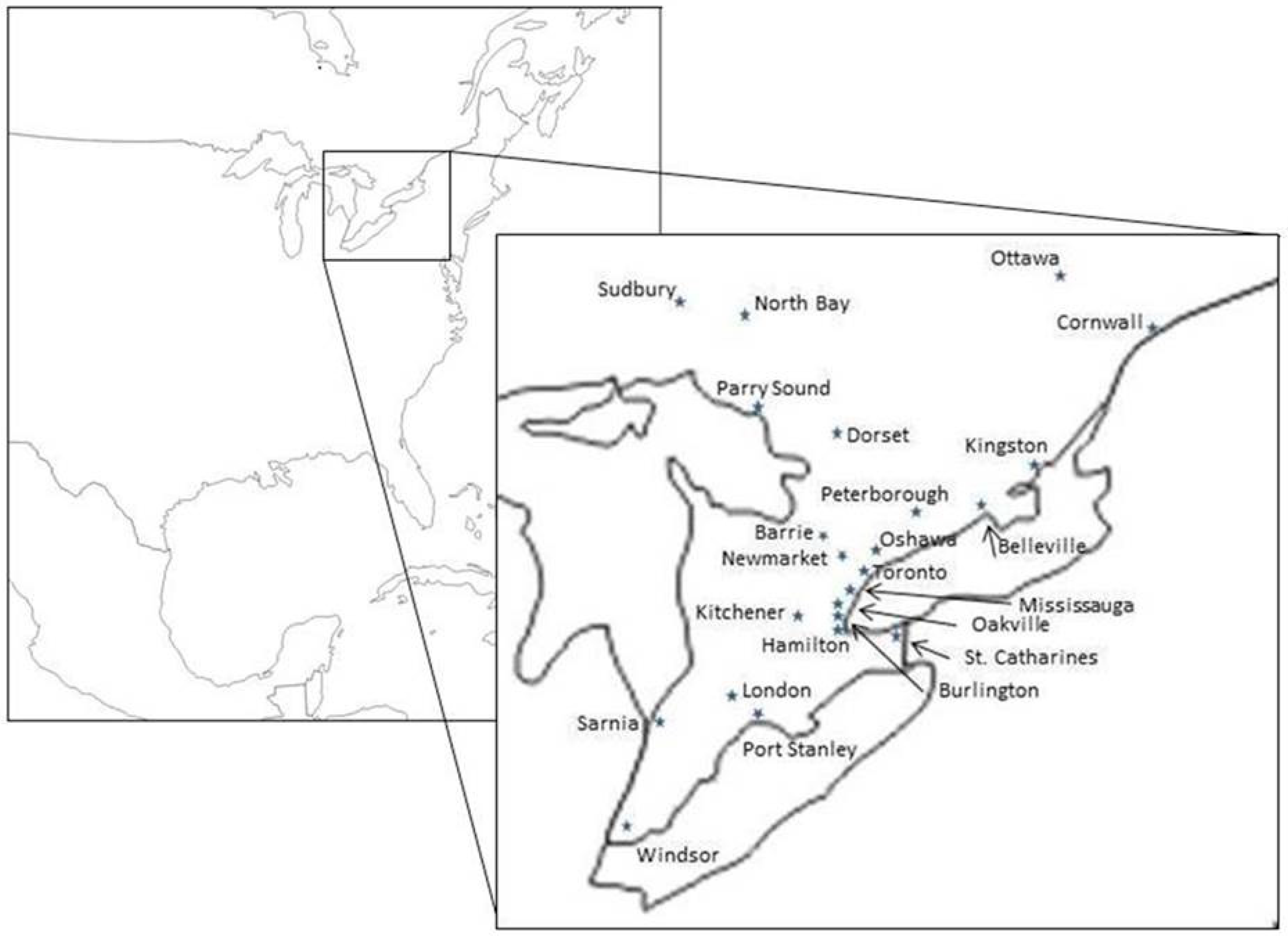
2. Data and Methods
3. Results and Discussion
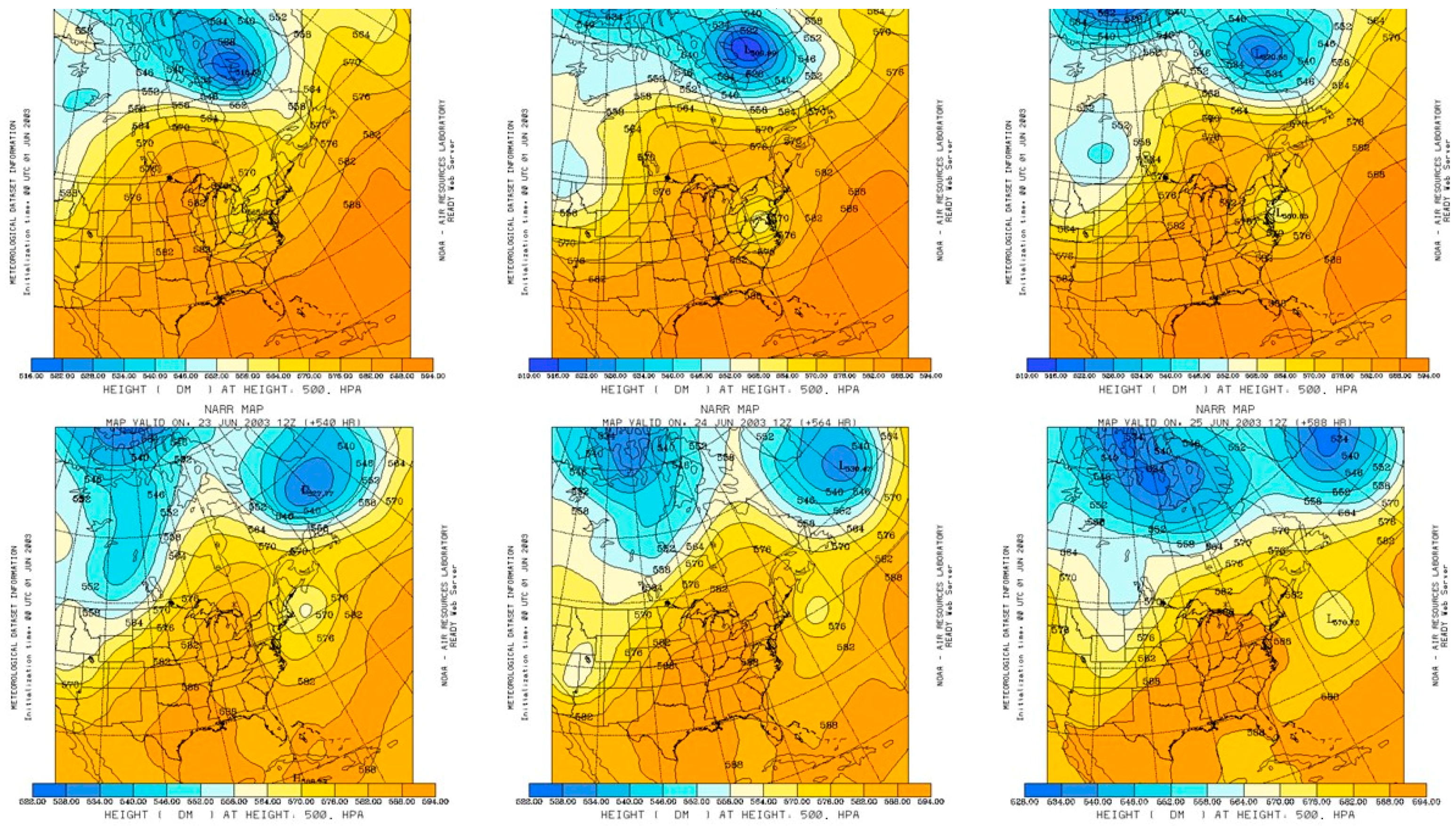
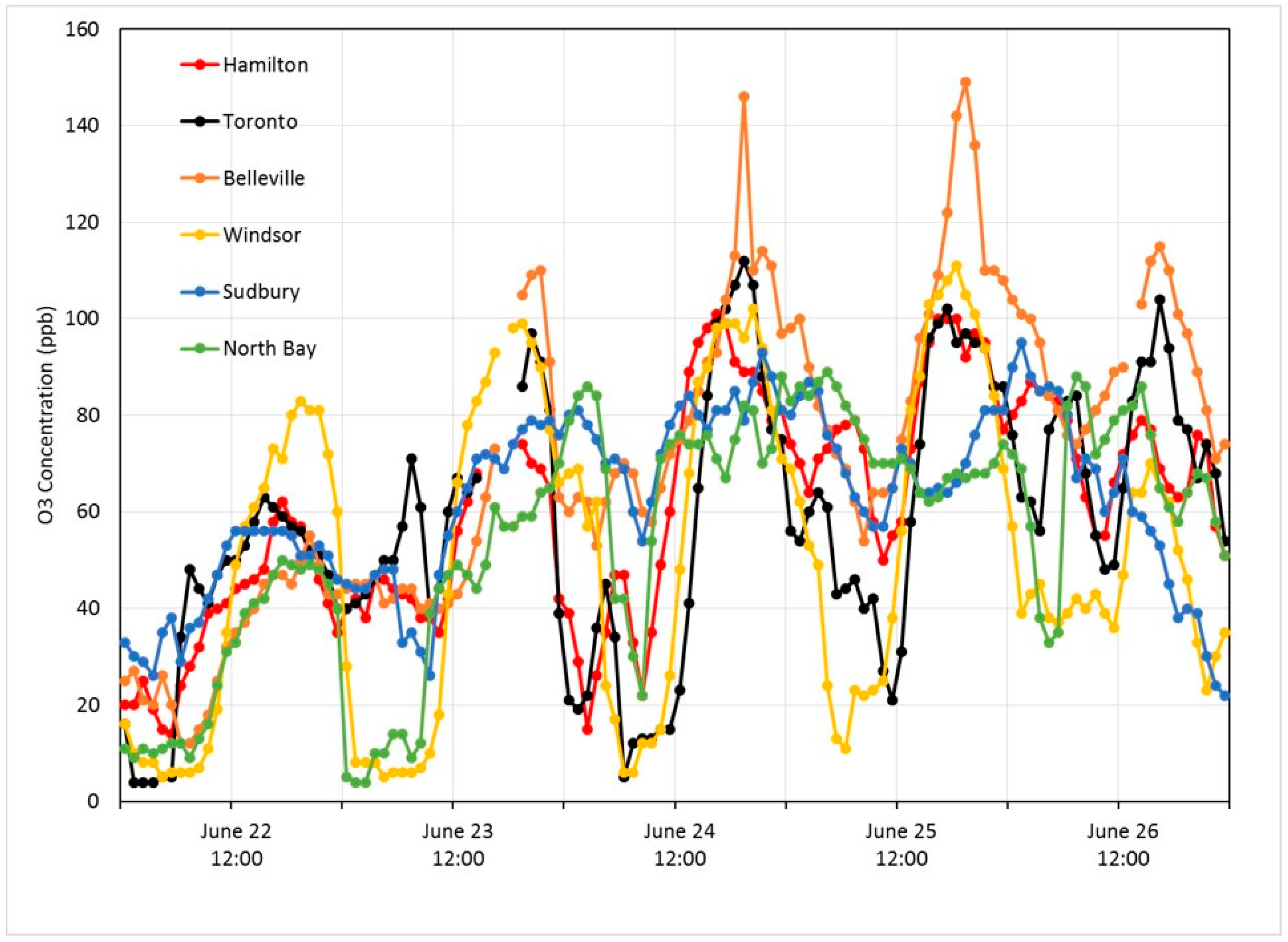
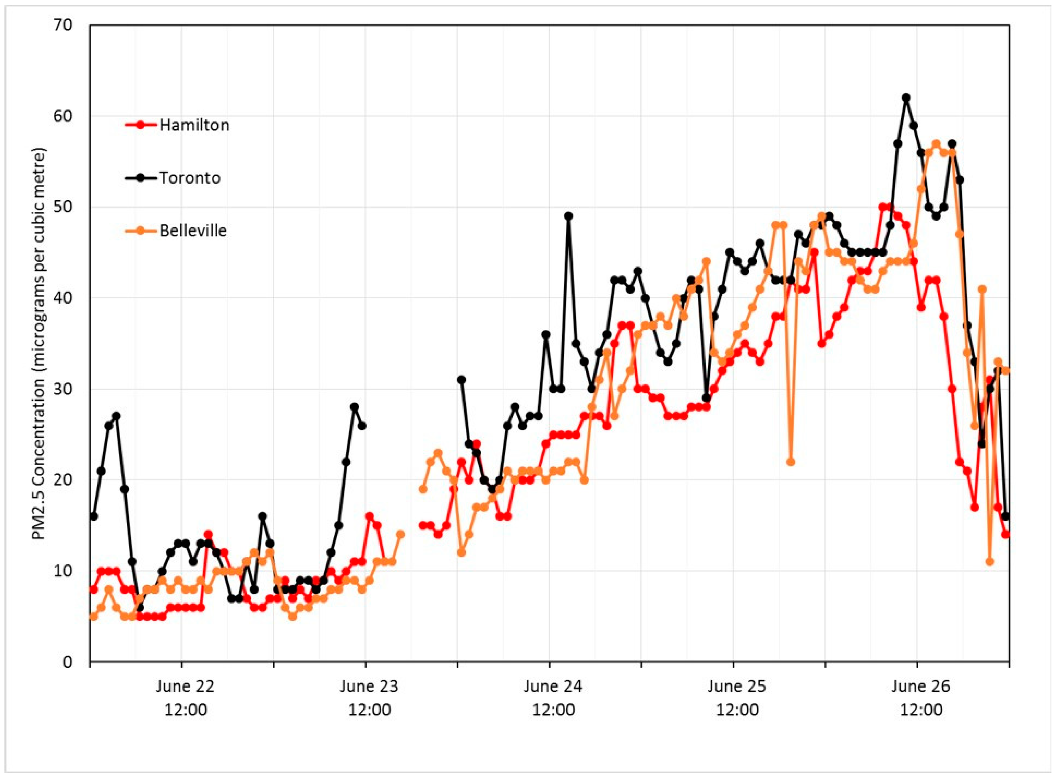
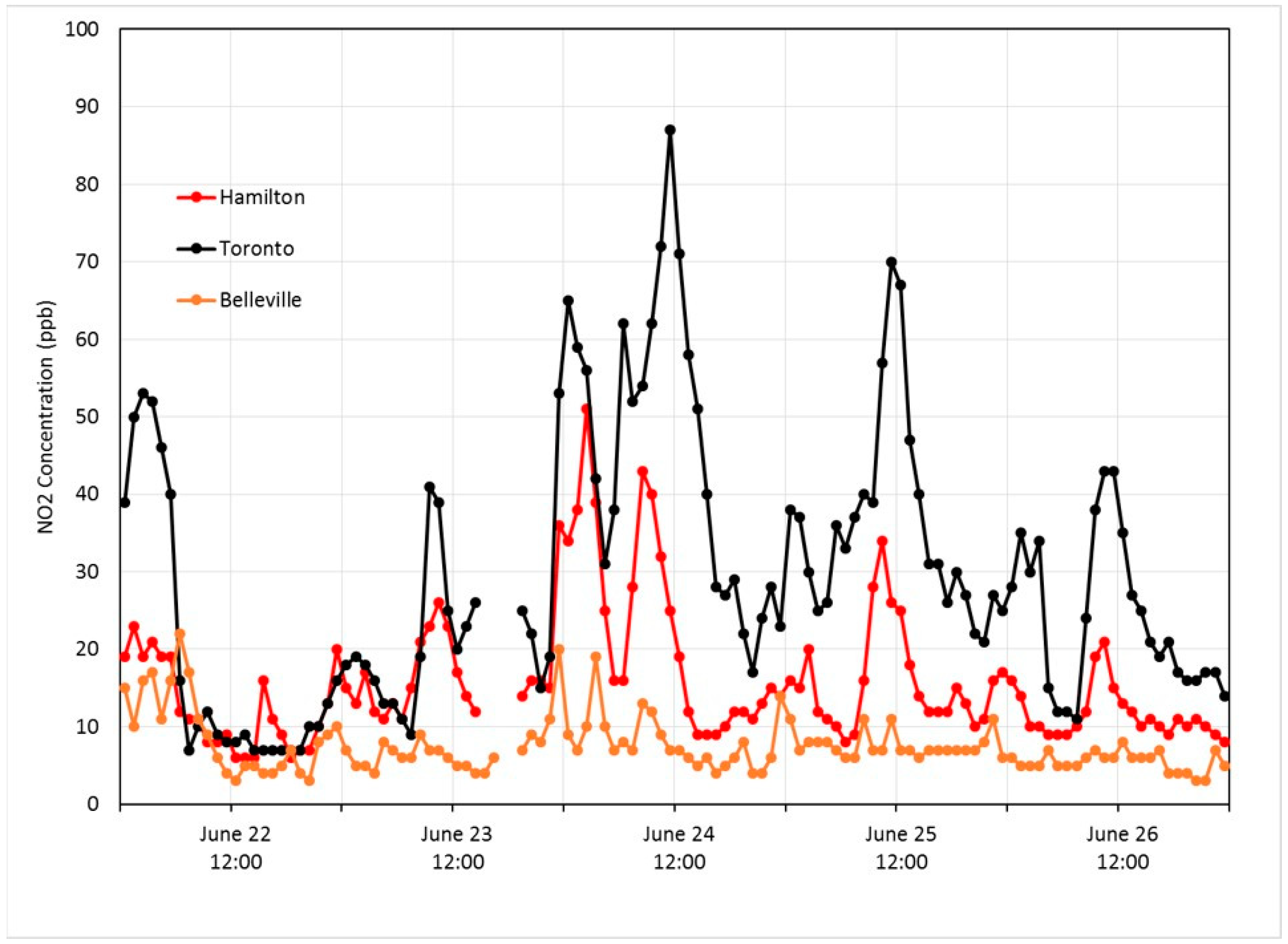
3.1. Example of 22–25 June 2003
3.1.1. Introduction
3.1.2. Synoptic Description
3.1.3. Discussion
3.1.4. Summary
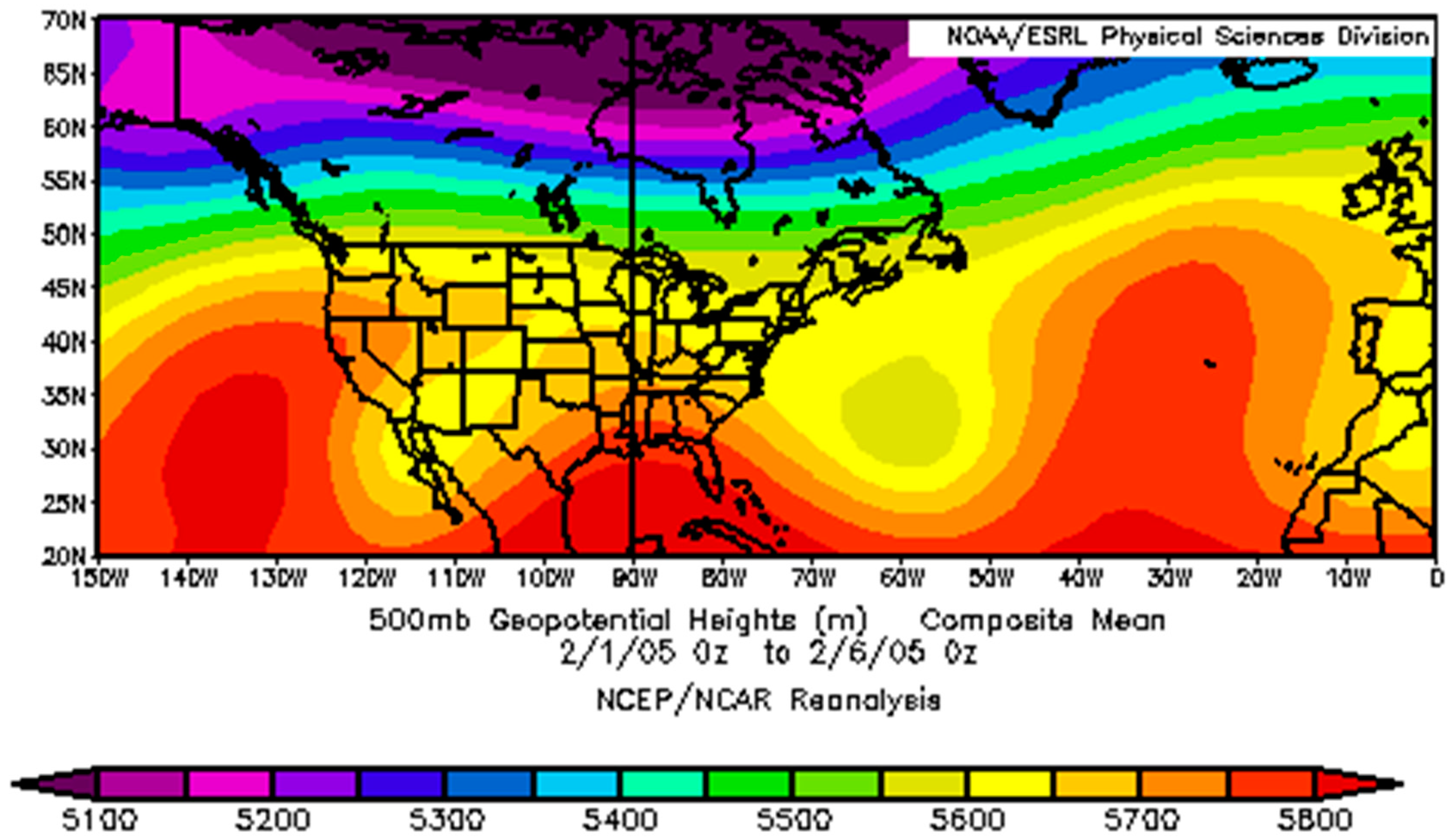
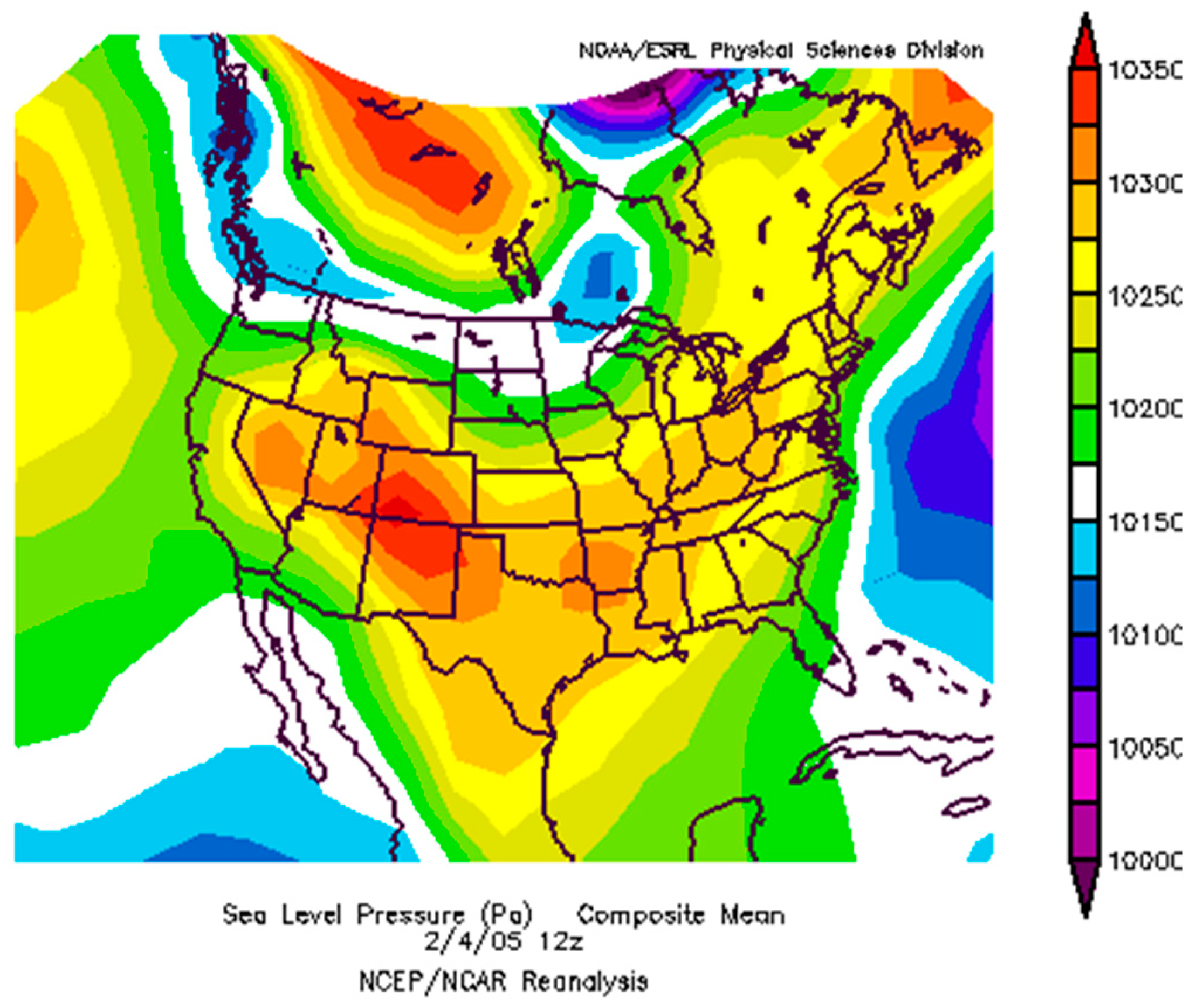
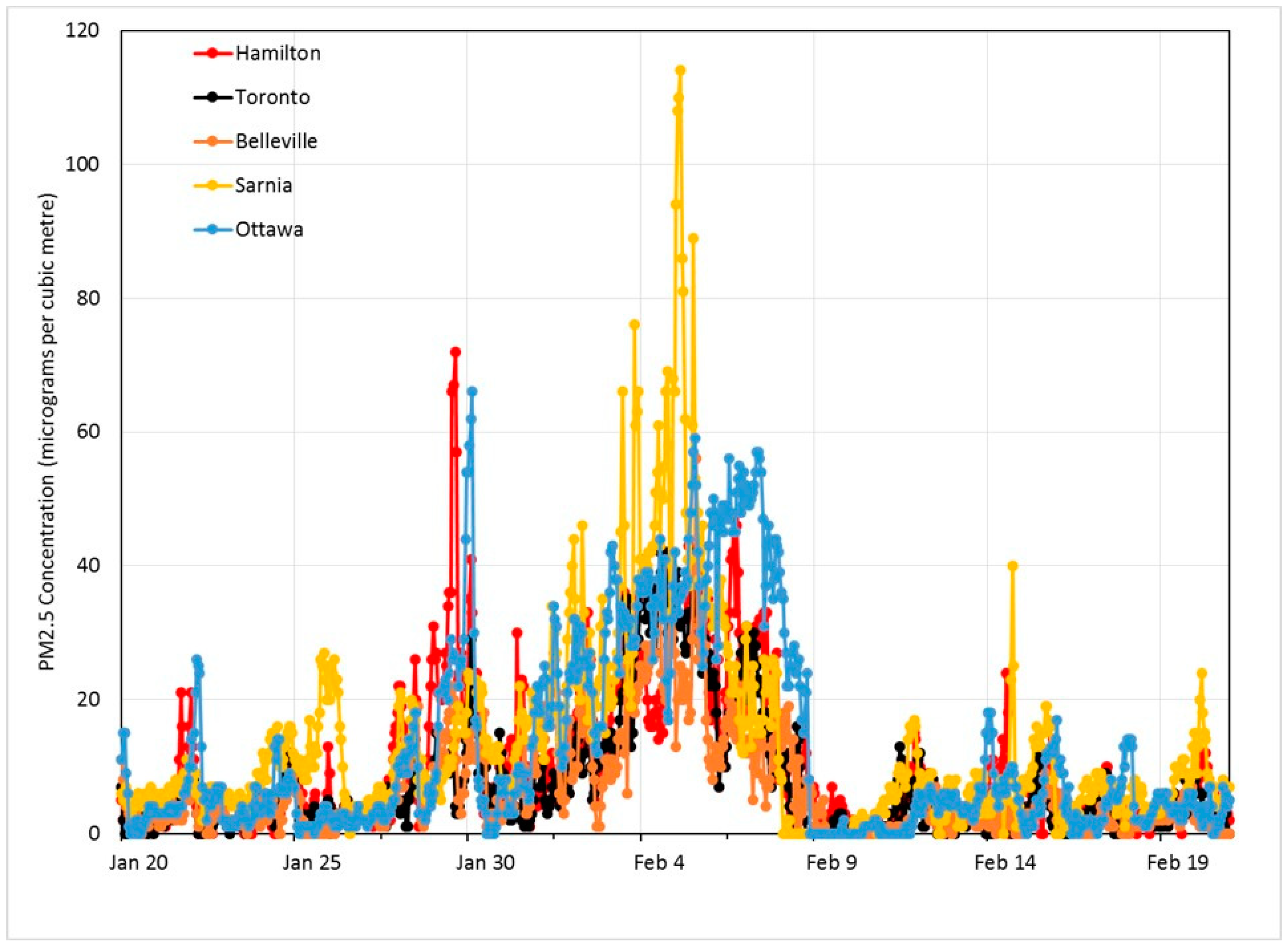
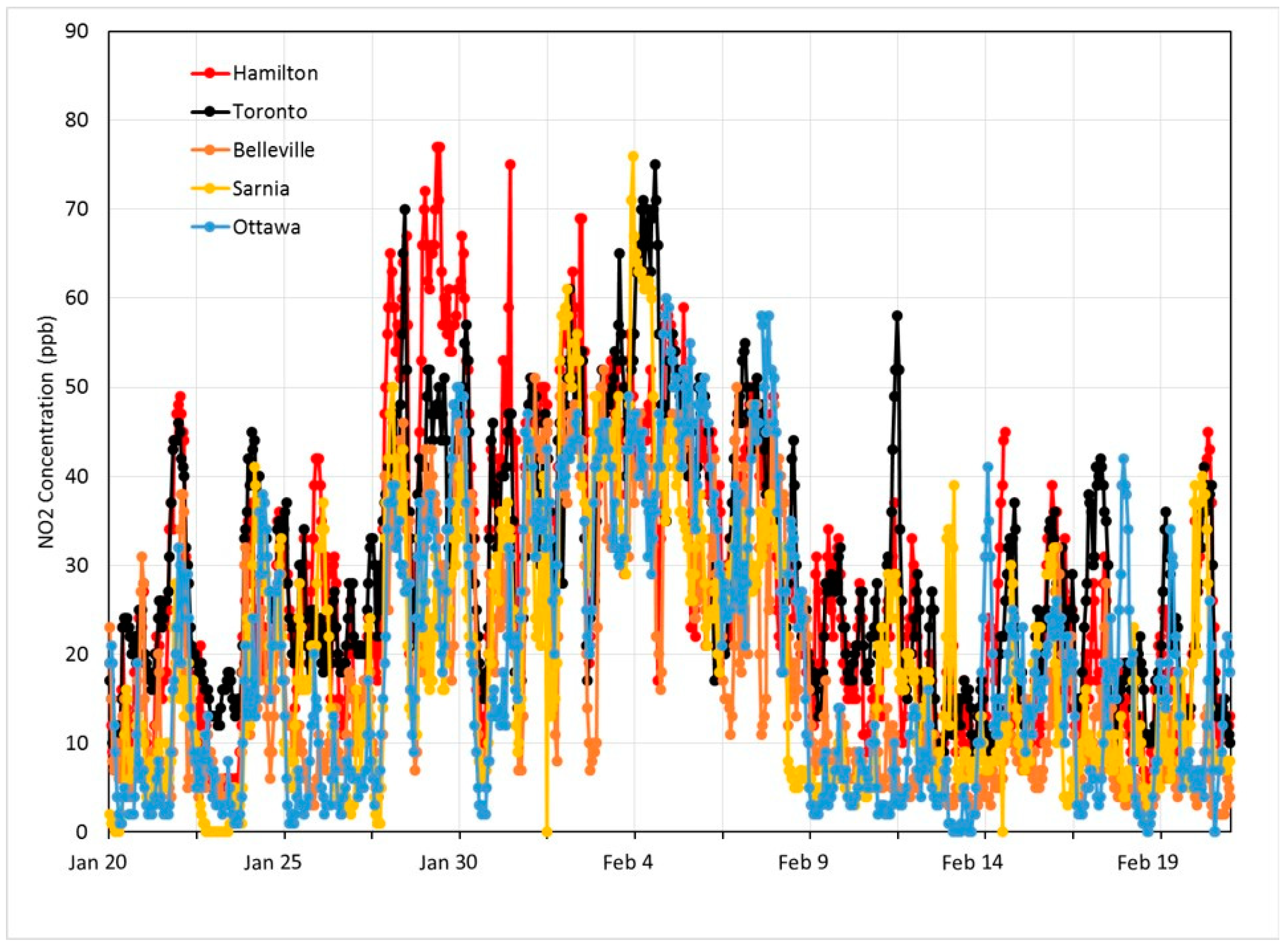
3.2. Example of 2–7 February 2005
3.2.1. Introduction
3.2.2. Synoptic Description
3.2.3. Discussion
3.2.4. Summary
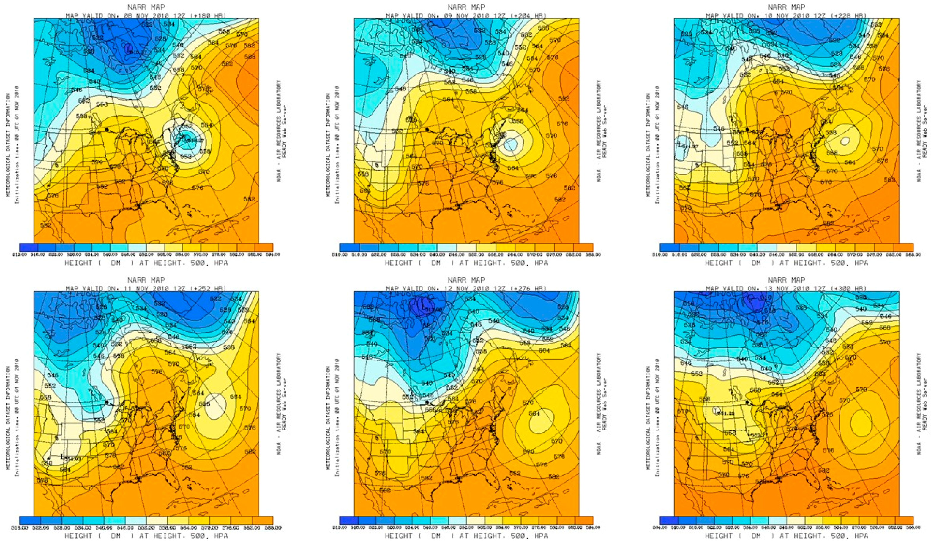
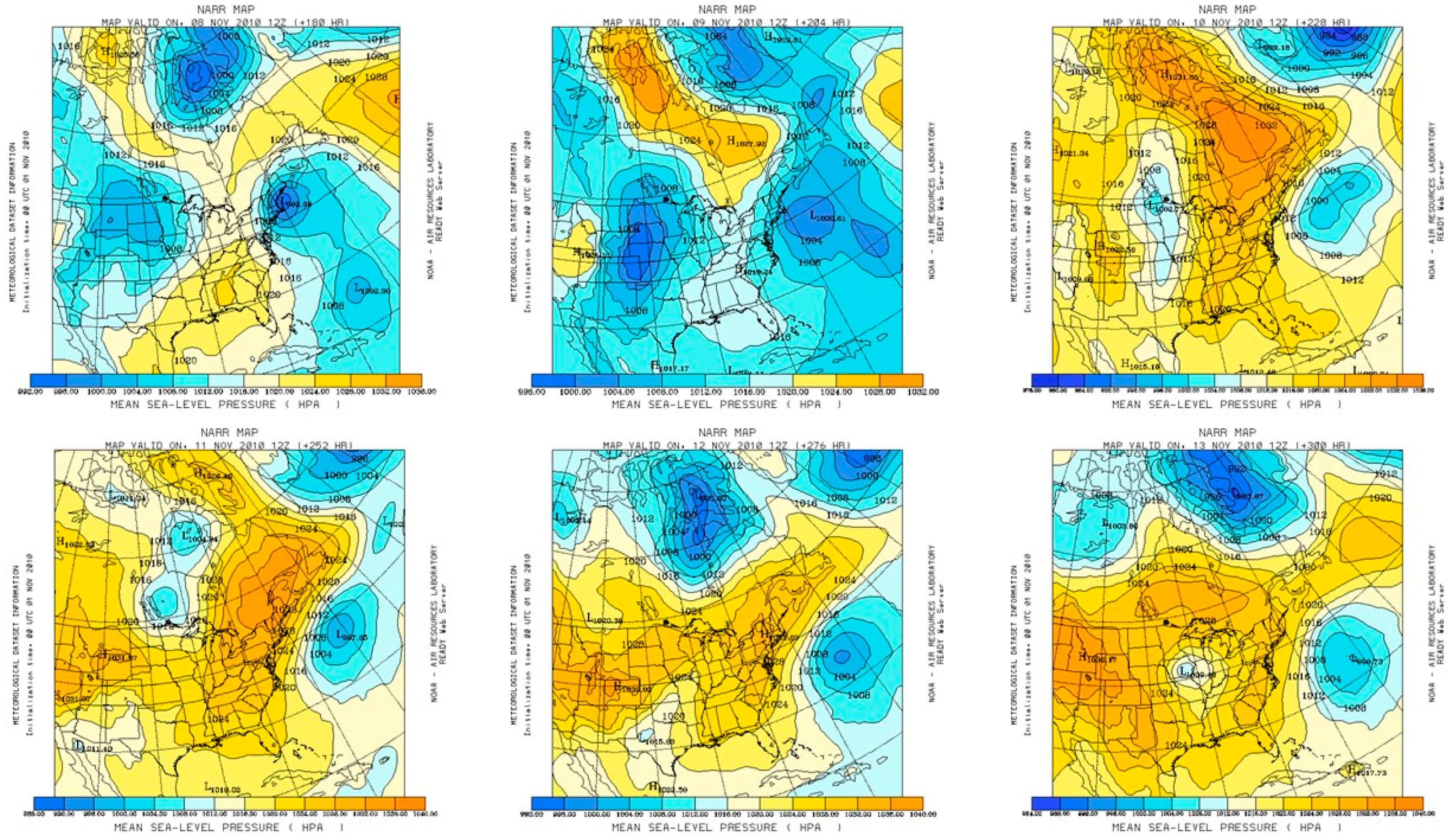
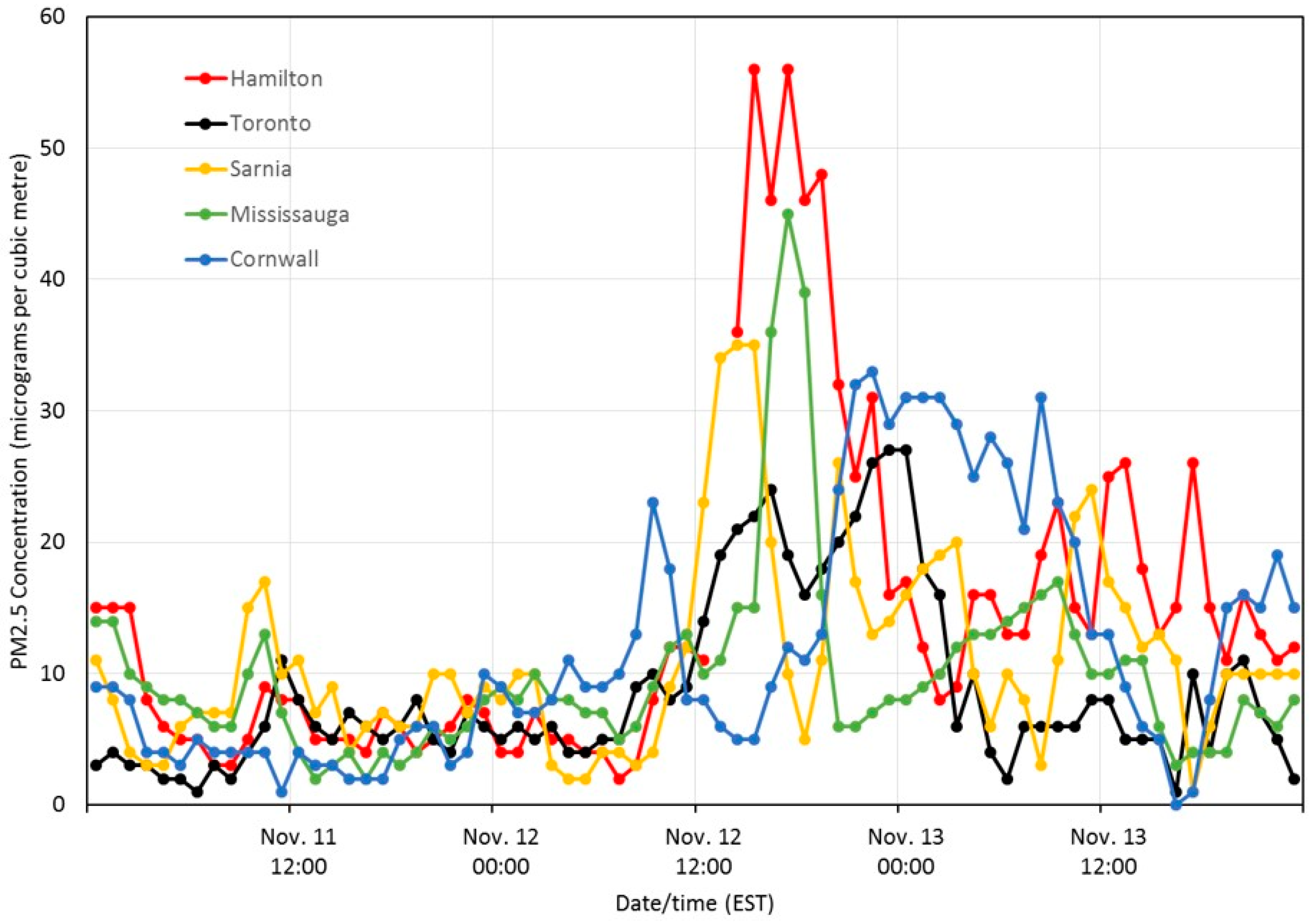
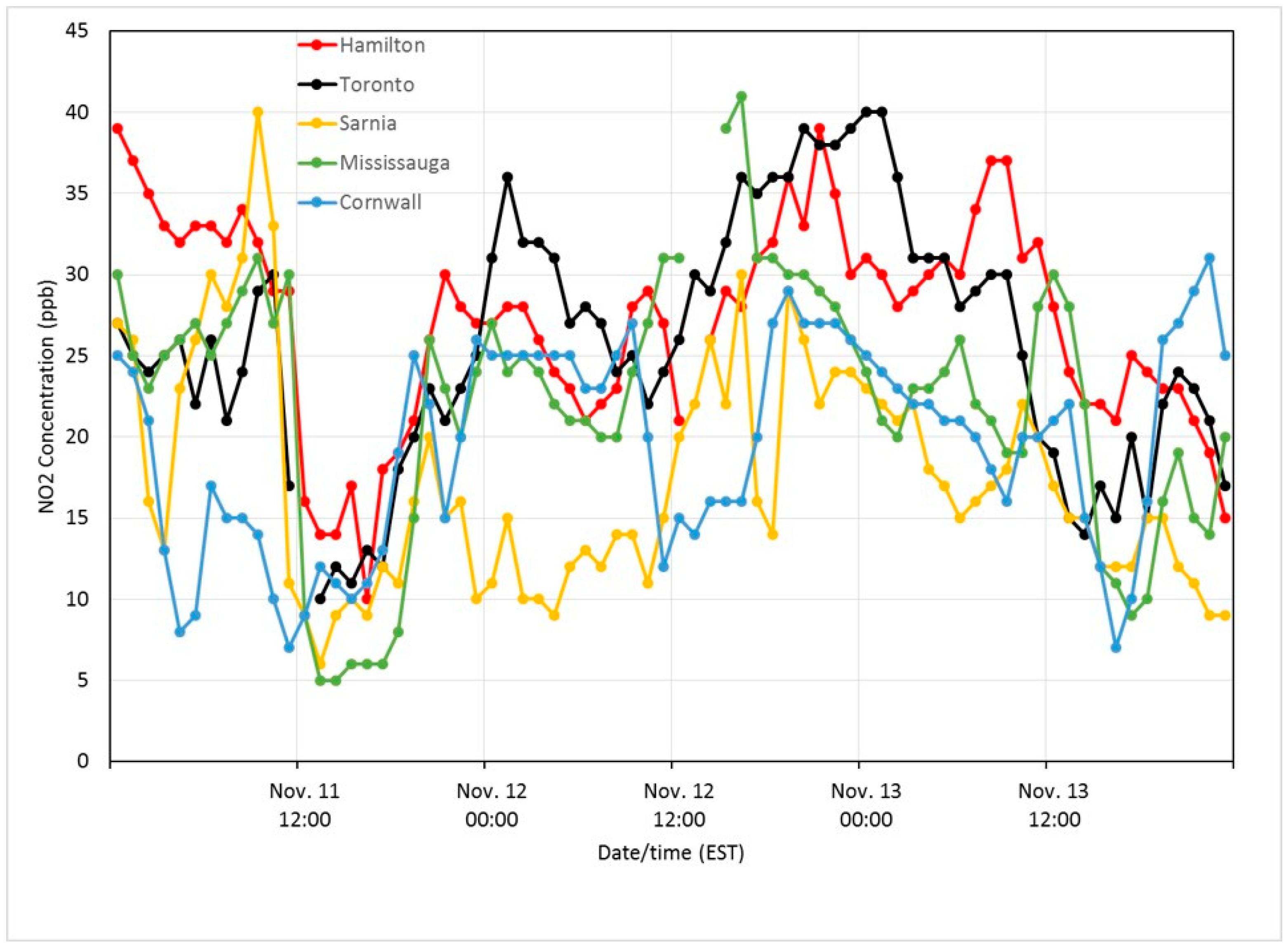
3.3. Example of 12 November 2010
3.3.1. Introduction
3.3.2. Synoptic Description
3.3.3. Discussion
3.3.4. Summary
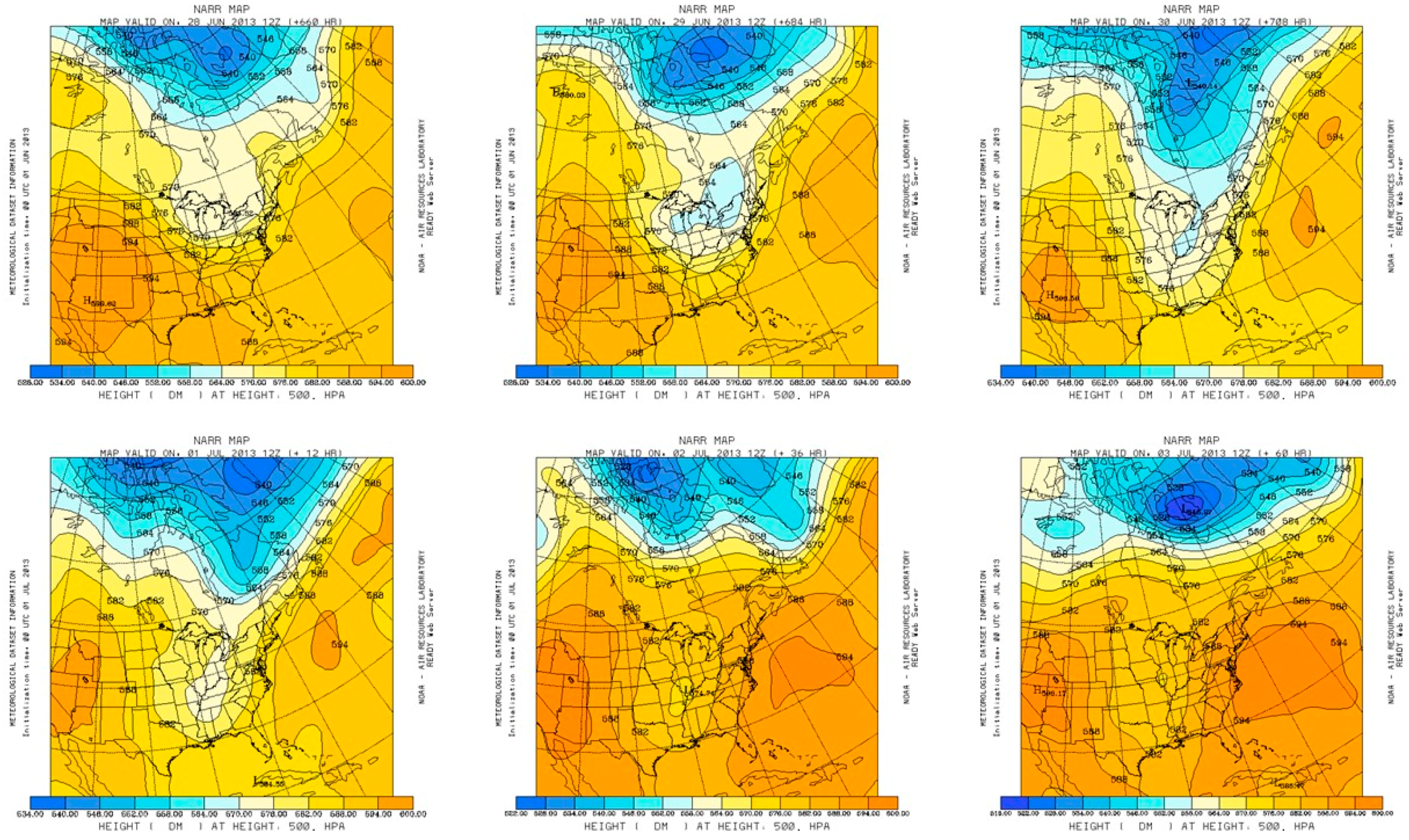
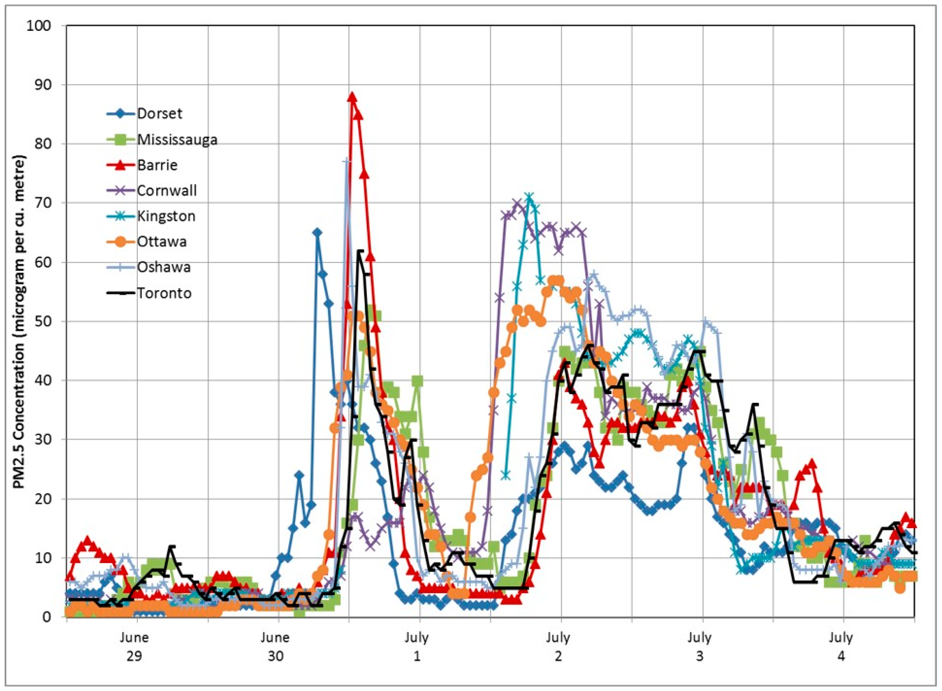
3.4. Example of 1 July 2013
3.4.1. Introduction
3.4.2. Synoptic Description
3.4.3. Discussion
3.4.4. Summary
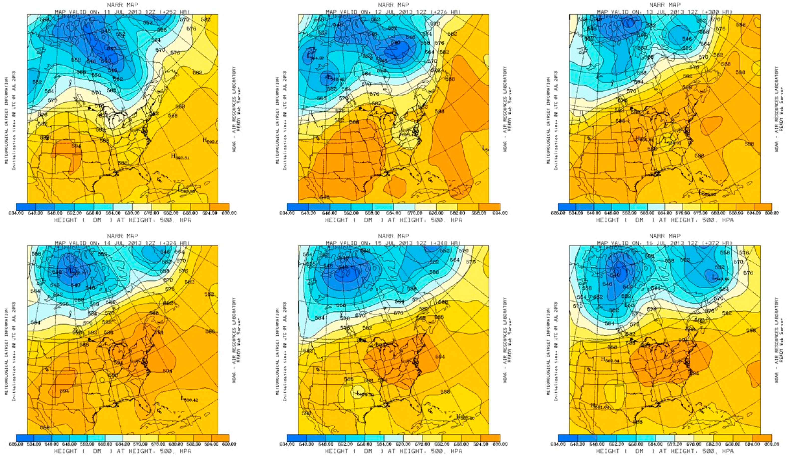
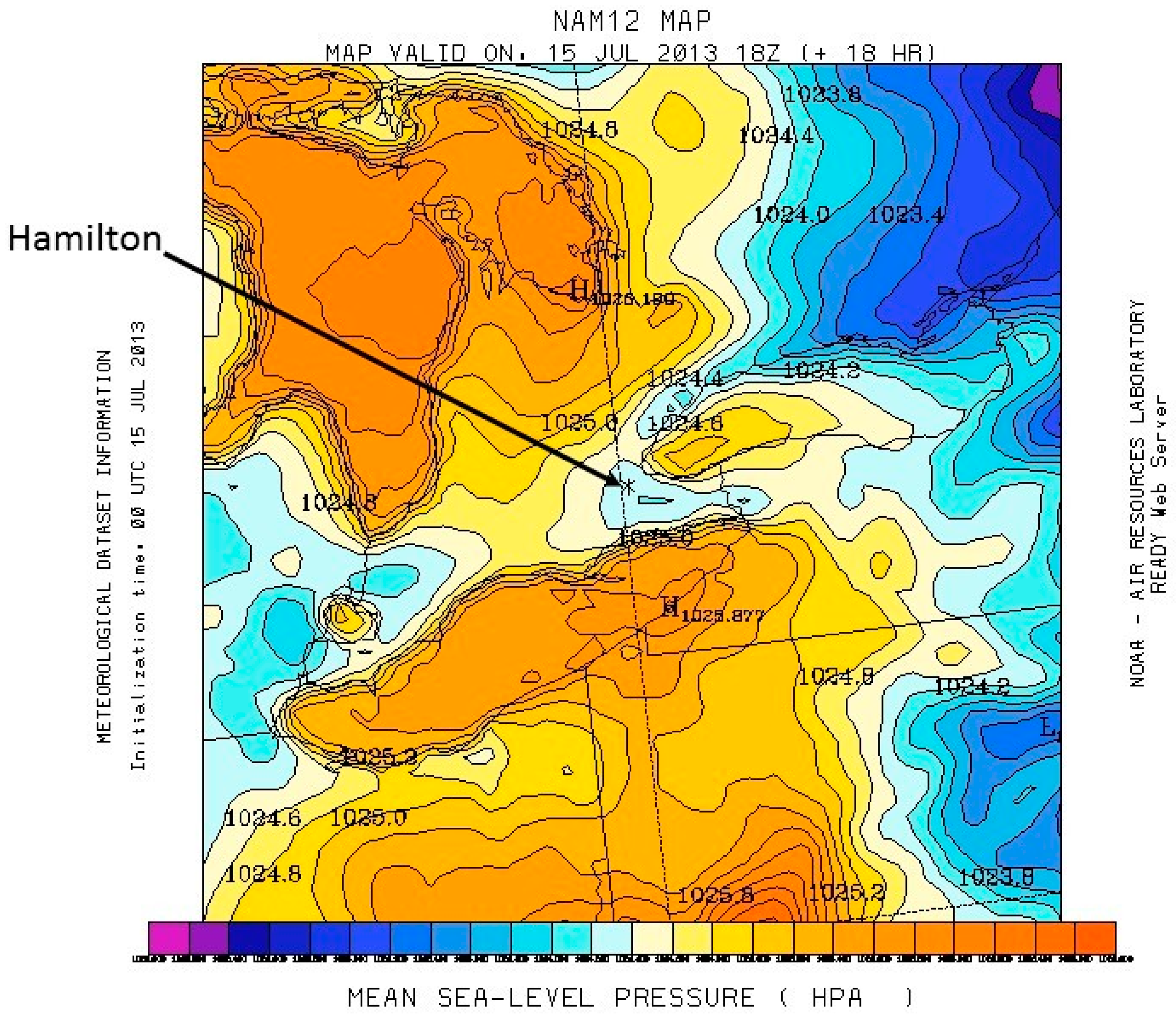
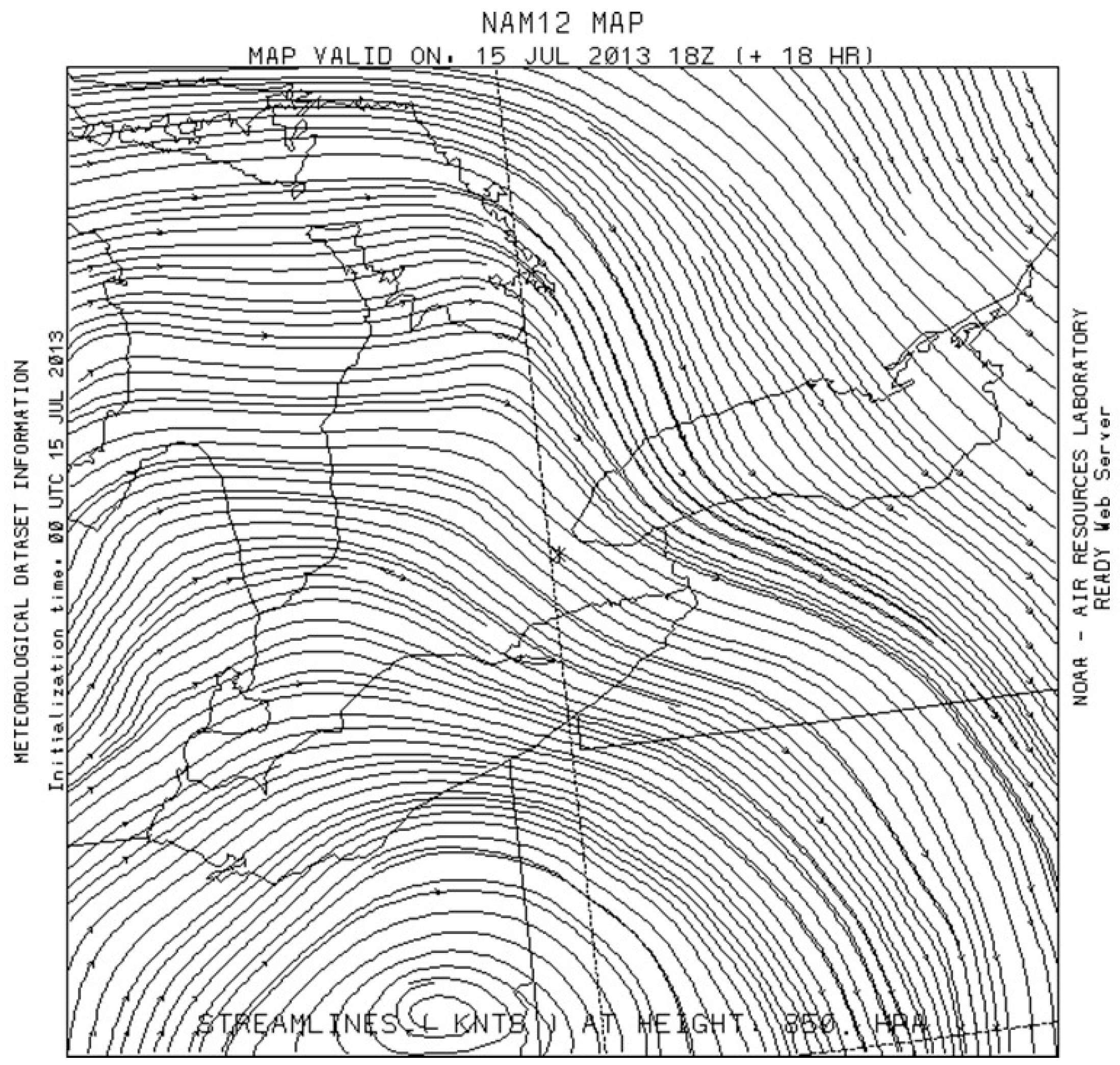
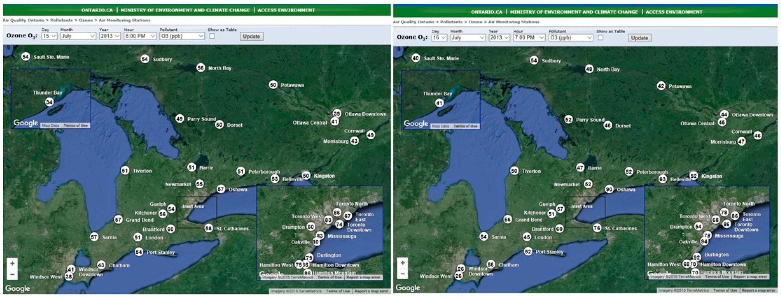
3.5. Example of 15 July 2013
3.5.1. Introduction
3.5.2. Synoptic Description
3.5.3. Discussion
3.5.4. Summary
4. Conclusions
Supplementary Materials
Conflicts of Interest
References
- Carrera, M.L.; Higgins, R.W.; Kousky, V.E. Downstream weather impacts associated with atmospheric blocking over the northeast Pacific. J. Clim. 2004, 17, 4823–4839. [Google Scholar] [CrossRef]
- Charney, J.G.; Shukla, J.; Mo, K.C. Comparison of a Barotropic Blocking Theory with Observation. J. Atmos. Sci. 1981, 38, 762–779. [Google Scholar] [CrossRef]
- Barriopedro, D.; Garcia-Herrera, R.; Lupo, A.; Hernandez, E.A. Climatology of northern hemisphere blocking. J. Clim. 2006, 19, 1042–1063. [Google Scholar] [CrossRef]
- Grose, W.L.; Hoskins, B.J. On the influence of orography on large-scale atmospheric flow. J. Atmos. Sci. 1979, 36, 223–234. [Google Scholar] [CrossRef]
- Hakkinen, S.; Rhines, P.; Worthen, D. Atmospheric blocking and Atlantic Multidecadal Ocean variability. Science 2011, 334, 655–659. [Google Scholar] [CrossRef] [PubMed]
- Peings, Y.; Magnusdottir, G. Forcing of the wintertime atmospheric circulation by the multidecadal fluctuations of the North Atlantic ocean. Environ. Res. Lett. 2014, 9, 034018. [Google Scholar] [CrossRef]
- Shabbar, A.; Huang, J.; Higuchi, J. The relationship between the wintertime north Atlantic oscillation and blocking episodes in the north Atlantic. Int. J. Climatol. 2001, 21, 355–369. [Google Scholar] [CrossRef]
- Barriopedro, D.; Calvo, N. On the relationship between ENSO, stratospheric sudden warmings, and blocking. J. Clim. 2014, 27, 4704–4720. [Google Scholar] [CrossRef]
- Cassou, C. Intraseasonal interaction between the Madden-Julian Oscillation and the north Atlantic Oscillation. Nat. Lett. 2008, 455, 523–527. [Google Scholar] [CrossRef] [PubMed]
- Henderson, S.A.; Maloney, E.D.; Barnes, E.A. The Influence of the Madden–Julian Oscillation on northern hemisphere winter blocking. J. Clim. 2016, 29, 4597–4616. [Google Scholar] [CrossRef]
- Barriopedro, D.; García-Herrera, R.; Huth, R. Solar modulation of Northern Hemisphere winter blocking. J. Geophys. Res. Atmos. 2008, 113, D14118. [Google Scholar] [CrossRef]
- Mitchell, D.M.; Gray, L.J.; Anstey, J.; Baldwin, M.P.; Charlton-Perez, A.J. The influence of stratospheric vortex displacements and splits on surface climate. J. Clim. 2013, 26, 2668–2682. [Google Scholar] [CrossRef]
- Glecker, P.J.; Santer, B.D.; Domingues, C.M.; Pierce, D.W.; Barnett, T.P.; Church, J.A.; Taylor, K.E.; AchutaRao, K.M.; Boyer, T.P.; Ishii, M.; et al. Human-induced global ocean warming on multidecadal timescales. Nat. Clim. Chang. 2012, 2, 524–529. [Google Scholar] [CrossRef]
- Meehl, G.A.; Washington, W.M.; Wigley, T.M.L.; Arblaster, J.M.; Dai, A. Solar and Greenhouse Gas Forcing and Climate Response in the Twentieth Century. J. Clim. 2003, 16, 426–444. [Google Scholar] [CrossRef]
- Radel, G.; Mauritsen, T.; Stevens, B.; Dommenget, D.; Matei, D.; Bellomo, K.; Clement, A. Amplification of El Nino by cloud longwave coupling to atmospheric circulation. Nat. Geosci. 2016, 9, 106–110. [Google Scholar] [CrossRef]
- Clement, A.C.; Burgman, R.; Norris, J.R. Observational and model evidence for positive low-level cloud feedback. Science 2009, 324, 450–464. [Google Scholar] [CrossRef] [PubMed]
- Sutton, R.T.; Allen, M.R. Decadal predictability of North Atlantic sea surface temperature and climate. Nature 1997, 388, 563–567. [Google Scholar] [CrossRef]
- Commou, D.; Lehmann, J.; Beckmann, J. The weakening summer circulation in the northern hemisphere mid-latitudes. Sci. Express 2015, 348, 324–327. [Google Scholar] [CrossRef] [PubMed]
- Francis, J.; Skific, N. Evidence linking rapid Arctic warming to mid-latitude weather patterns. Philos. Trans. R. Soc. A 2015, 373, 20140170. [Google Scholar] [CrossRef] [PubMed]
- Barnes, E. Revisiting the evidence linking Arctic amplification to extreme weather in midlatitudes. Geophys. Res. Lett. 2013, 40, 4734–4739. [Google Scholar] [CrossRef]
- Kennedy, D.; Parker, T.; Woolings, T.; Harvey, B.; Shaffrey, L. The response of high-impact blocking weather systems to climate change. Geophys. Res. Lett. 2016, 43, 7250–7258. [Google Scholar] [CrossRef]
- Rex, D.F. Blocking action in the middle troposphere and its effect upon regional climate. 1. An aerological study of blocking action. Tellus 1950, 2, 196–211. [Google Scholar] [CrossRef]
- Treidl, R.; Birch, E.; Sajecki, P. Blocking action in the northern hemisphere: A climatological study. Atmos. Ocean 1981, 19, 1–23. [Google Scholar] [CrossRef]
- White, W.B.; Clark, N.E. On the development of blocking ridge activity over the central North Pacific. J. Atmos. Sci. 1975, 32, 489–502. [Google Scholar] [CrossRef]
- Dole, R.M.; Gordon, N.D. Persistent anomalies of the extra-tropical Northern Hemisphere wintertime circulation: Geographical distribution and regional persistence characteristics. Mon. Weather Rev. 1983, 111, 1567–1586. [Google Scholar] [CrossRef]
- Lejenas, H.; Oakland, H. Characteristics of northern hemisphere blocking as determined from long time series of observational data. Tellus 1983, 35A, 350–362. [Google Scholar] [CrossRef]
- Tibaldi, S.; Molteni, F. On the operational predictability of blocking. Tellus 1990, 42A, 343–365. [Google Scholar] [CrossRef]
- McKendry, I.G. Synoptic circulation and summertime ground-level ozone concentrations at Vancouver, British Columbia. J. Appl. Meteorol. 1994, 33, 627–641. [Google Scholar] [CrossRef]
- Shahgedanova, M.; Burt, T.P.; Davies, T.D. Synoptic climatology of air pollution in Moscow. Theor. Appl. Climatol. 1998, 51, 85–102. [Google Scholar] [CrossRef]
- Jiang, N.; Dirks, K.; Luo, K. Effects of local, synoptic and large-scale climate conditions on daily nitrogen dioxide concentrations in Auckland, New Zealand. Int. J. Climatol. 2013, 34, 1883–1897. [Google Scholar] [CrossRef]
- Kampa, M.; Castanas, E. Human health effects of air pollution. Environ. Pollut. 2008, 151, 362–367. [Google Scholar] [CrossRef] [PubMed]
- Holloway, A.M.; Wayne, R.P. Atmospheric Chemistry; RCS Publishing: Cambridge, UK, 2010; pp. 101–120. ISBN 978-1-84755-807-7. [Google Scholar]
- Jacob, D.J. Introduction to Atmospheric Chemistry; Princeton University Press: Princeton, NJ, USA, 1999; pp. 200–216. ISBN 0-691-00185-5. [Google Scholar]
- Brook, J.R.; Makar, P.A.; Sills, D.; Hayden, K.L.; McLaren, R. Exploring the nature of air quality over southwestern Ontario: Main findings from the Border Air Quality and Meteorology Study. Atmos. Chem. Phys. 2013, 13, 10461–10482. [Google Scholar] [CrossRef]
- Yap, D.; Reid, N.; De Brou, G.; Bloxam, R. Transboundary Air Pollution in Ontario. Ontario Ministry of the Environment. 2005. Available online: http://www.airqualityontario.com/downloads/TransboundaryAirPollutionInOntario2005.pdf (accessed on 14 May 2018).
- Kalnay, E.; Kanamitsu, M.; Kistler, R.; Collins, W.; Deaven, D.; Gandin, L.; Iredell, M.; Saha, S.; White, G.; Woollen, J.; et al. The NCEP/NCAR 40-Year Reanalysis Project. Bull. Am. Meteorol. Soc. 1996, 77, 437–471. [Google Scholar] [CrossRef]
- Dempsey, F. Forest Fire Effects on Air Quality in Ontario: Evaluation of Several Recent Examples. Bull. Am. Meteorol. Soc. 2013, 94, 1059–1064. [Google Scholar] [CrossRef]
- Pfister, G.G.; Wiedinmyer, C.; Emmons, L.K. Impacts of the fall 2007 California wildfires on surface ozone: Integrating local observations with global model simulations. Geophys. Res. Lett. 2008, 35, L19814. [Google Scholar] [CrossRef]


| City | Latitude | Longitude | Population (2016) (Data from Statistics Canada) | Urban or Rural Environment near Monitoring Station | Affected by Lake Breezes? |
|---|---|---|---|---|---|
| Barrie | 44°22’56.5” | −79°42’08.3” | 141,000 | urban | N |
| Belleville | 44°09’01.9” | −77°23’43.8” | 51,000 | urban | Y |
| Cornwall | 45°01’04.7” | −74°44’06.8” | 47,000 | urban | N |
| Dorset | 45°13’27.4” | −78°55’58.6” | <1000 | rural | N |
| Hamilton | 43°15’28.0” | −79°51’42.0” | 537,000 | urban | Y |
| Kingston | 44°13’11.5” | −76°31’16.1” | 124,000 | urban | Y |
| Mississauga | 43°32’49.1” | −79°39’31.3” | 722,000 | urban | Y |
| North Bay | 46°19’23.5” | −79°26’57.4” | 52,000 | urban | N |
| Oshawa | 43°56’45.4” | −78°53’41.7” | 159,000 | urban | Y |
| Ottawa | 45°26’03.6” | −75°40’33.6” | 934,000 | urban | N |
| Sarnia | 42°58’56.2” | −82°24’18.3” | 72,000 | urban | Y |
| Sudbury | 46°29’31.0” | −81°00’11.2” | 22,000 | urban | N |
| Toronto | 43°39’46.7” | −79°23’17.2” | 2,732,000 | urban | Y |
| Windsor | 42°18’56.8” | −83°02’37.2” | 217,000 | urban | Y |
| Block Type | Season | Pollutants Affected | Notes |
|---|---|---|---|
| Ridge over southern Ontario-eastern U.S. | summer | O3, NO2, PM2.5 | Hot, humid, stagnant weather conditions are typical |
| Ridge over southern Ontario-eastern U.S. | winter | PM2.5, NO2 | Important when a block persists long enough to cause stagnating conditions |
| Ridge over southern Ontario-eastern U.S. | summer | O3 | Retrogressing ridge over southern Ontario may result in enhanced O3 formation in near-lake marine layers and strong lake breeze circulations |
| Mesoscale ridge over southern Ontario | Autumn (during periods when air temperatures over land and lakes are similar) | PM2.5, NO2 | Coincides with nocturnal inversions persisting during the morning (or day) and fog which may contribute to PM2.5 formation and restrict insolation |
| Low pressure trough over southern Great Lakes region | Summer (during active wildfire periods) | PM2.5 (sometimes O3, NO2) | Dependent on locations of wildfires |
© 2018 by the author. Licensee MDPI, Basel, Switzerland. This article is an open access article distributed under the terms and conditions of the Creative Commons Attribution (CC BY) license (http://creativecommons.org/licenses/by/4.0/).
Share and Cite
Dempsey, F. A Survey of Regional-Scale Blocking Patterns and Effects on Air Quality in Ontario, Canada. Atmosphere 2018, 9, 226. https://doi.org/10.3390/atmos9060226
Dempsey F. A Survey of Regional-Scale Blocking Patterns and Effects on Air Quality in Ontario, Canada. Atmosphere. 2018; 9(6):226. https://doi.org/10.3390/atmos9060226
Chicago/Turabian StyleDempsey, Frank. 2018. "A Survey of Regional-Scale Blocking Patterns and Effects on Air Quality in Ontario, Canada" Atmosphere 9, no. 6: 226. https://doi.org/10.3390/atmos9060226
APA StyleDempsey, F. (2018). A Survey of Regional-Scale Blocking Patterns and Effects on Air Quality in Ontario, Canada. Atmosphere, 9(6), 226. https://doi.org/10.3390/atmos9060226