Modelling of Basin Wide Daily Evapotranspiration with a Partial Integration of Remote Sensing Data

1. Introduction

A discrepancy between water availability and water demand is present continuously and globally, with food production making 70% of all water withdrawals [1]. Spatial and temporal variations of available water resources are altered by climate change in many river basins worldwide. Droughts in Europe have incurred a total cost of €100 billion over the past 30 years with a sharp upward trend, so the average costs from droughts have quadrupled [2]. The Mediterranean and the Danube regions in Europe are recognized as being highly vulnerable to droughts [1] with two recent long term droughts, in 2003 and 2015.

Evapotranspiration (ET) is major water balance output component in river basins [3,4] and greatly influences the hydrological cycle and the energy balance of the land surface [5]. ET is governed by numerous physical factors and is the most difficult water balance component to measure or to estimate. Evaporation is influenced by solar energy, amount of water and potential water vapour uplift between the surface and the atmosphere, and transpiration is predominantly influenced by soil moisture deficit along with vegetation cover, vapour pressure gradient and energy supply. Additional influences on the transpiration rate are soil conductivity, depth of the rooting zone, water logging, water salinity, environmental aspects, cultivation practices, crop development, etc. [6,7,8]. Due to relatively slow development of ground based ET measurement techniques, there are still many challenges related to the spatio–temporal estimation of ET on a basin wide scale.

The direct measurements of ET are traditionally conducted by lysimeters on meteorological stations. Recently developed scintillometers are designed to provide data for surface flux analysis and hence can be used in ET estimation, but due to their complexity, expensive technology and licensing issues, scintillometer measurements are still not viable [9]. Additional ET measurement devices include neutron probes, Eddy covariance systems, Bowen ratio systems, sap flow systems, etc. Due to high installation, maintenance and monitoring costs, the datasets of all ground-based ET measurement techniques are either scarce or of limited duration (usually related to a specific project). All ground based measurements provide point ET information so the basin wide ET estimate can be significantly increased by the introduction of remote sensing inputs.

The point ET intensity can be continuously evaluated using numerous approaches for estimation of the actual ET (AET) or potential ET (PET). The standard AET methods are derived from the relationship between measured ET and climatological variables that directly or indirectly influence the process [10] and can be grouped into two categories: (i) methods based on combining PET estimate with ancillary data, such as precipitation measurements, various modelling parameters or crop coefficients [11]; and (ii) direct methods based on modifications of the Penman equation through linking equation parameters to water balance information or introducing ancillary parameters, such as soil saturation and land cover [12]. The direct AET estimation requires significant data input (solar radiation, air temperature, water surface, soil water content, water vapour pressure, air humidity and wind speed for evaporation estimates, and data on soil moisture, vegetation cover, vapour pressure gradient solar radiation, air temperature, air humidity and wind speed for transpiration estimates). On the other hand, the input data requirement for PET methods is much smaller and includes solar radiation, air temperature, air humidity, wind speed and alternatively reference surface, along with net and extraterrestrial radiations that can be computed, which makes PET the more frequently used ET approach in hydrological models [13]. All AET and PET methods provide spatially discrete ET estimates so the basin wide ET is greatly dependent on the number and spatial distribution of gauges in a basin.

The remote sensing based ET estimate is obtained from the formulation of surface energy balance by using the visible and thermal bands which are included in several approaches: SEBAL [6], METRIC [14], TSEB [15], S-SEBI [16], SEBS [7], STSEB [17], etc. The instantaneous latent heat flux of ET is calculated as a residual of the energy balance which is then converted into daily ET by different methods, such as the evaporative fraction or reference ET fraction. The remote sensing based ET estimates are available for local, regional and global scales and with high spatial resolution (up to 30 m), but their temporal resolution is still limited. Current high resolution platforms have a frequency of 16 days and are limited to clear sky conditions.

To enable efficient spatio–temporal evaluation of ET by using instantaneous satellite images, several approaches have been proposed—the combination of satellite images from two different platforms, the integration of satellite images into hydrological modelling and the combination of evaporative fraction (Λ) and point daily PET. Satellite images from two different platforms—temporally continuous images at lower grid resolution (i.e., MODIS at 1 km) and periodic images at higher grid resolution (i.e., Landsat at 30 m)—have been successfully integrated to allow continuous mapping of daily ET at a high spatial resolution [18,19]. Several studies have shown successful integration of satellite data into hydrological models for continuous ET estimates. Examples include a combination of PET and an improved relative ET factor through the use of SEBAL latent heat flux [20], a combination of temporary discrete TSEB ET and reflectance-based crop coefficient from the soil water content dynamic model [21], implementation of the dynamic leaf area index (LAI) from satellite images into the Variable Infiltration Capacity (VIC) model to correct the simulated ET [22], and a combination of a vegetation index based on remote sensing and the soil water balance model [23]. To obtain seasonal basin wide ET estimates, the combination of daily PET on meteorological stations and Λ was also suggested [6,14,24]. The Λ is implemented either as a single raster of instantaneous Λ, which is assumed to be “representative” for the analysed period [24], or as daily Λ from the temporal interpolation of a series of instantaneous Λ [14]. An evaluation of seasonal ET estimates using the suggested method was obtained by using different Λ: a single Λ from a “representative” image, linear interpolations of two consecutive Λ rasters and Λ interpolation using the cubic spline method. Scenarios for all different Λ provided satisfactory results, with similar standard errors in daily ET estimates of 20% [25].

Clearly there are various successful approaches for extrapolating and implementing instantaneous satellite images for obtaining spatio–temporal ET estimates, but they can be only implemented in periods with available satellite images. An attempt to apply the available satellite images acquired using thermal infrared band during periods with available satellite images (“historical” images) for the estimation of daily ET in periods with no satellite images available is developed and presented in the current study. This approach consists of combining daily PET rasters and an interpolated Λ raster which is derived from several instantaneous Λ and allows for daily ET estimation in periods with no satellite images available. The objective of this research is to test the proposed concept for estimating daily ET for periods with no satellite images available in the Krapina River Basin. Reliability is evaluated by comparing the obtained ET to the SEBAL ET estimates though the analysis of residuals (Δ), standard deviations of residuals (σ) and the Nash–Sutcliffe coefficient (NSE) over the basin. The proposed approach is also intercompared to daily ET rasters obtained by spatial interpolation of point PET estimates, which represents a simple approach for basin wide ET estimation for periods with no satellite images available. Measurements include 87 high resolution images from Landsat satellite and ET measurements on two lysimeters. The recommendation for a required number of input satellite images for reliable estimate of interpolated Λ is also investigated.

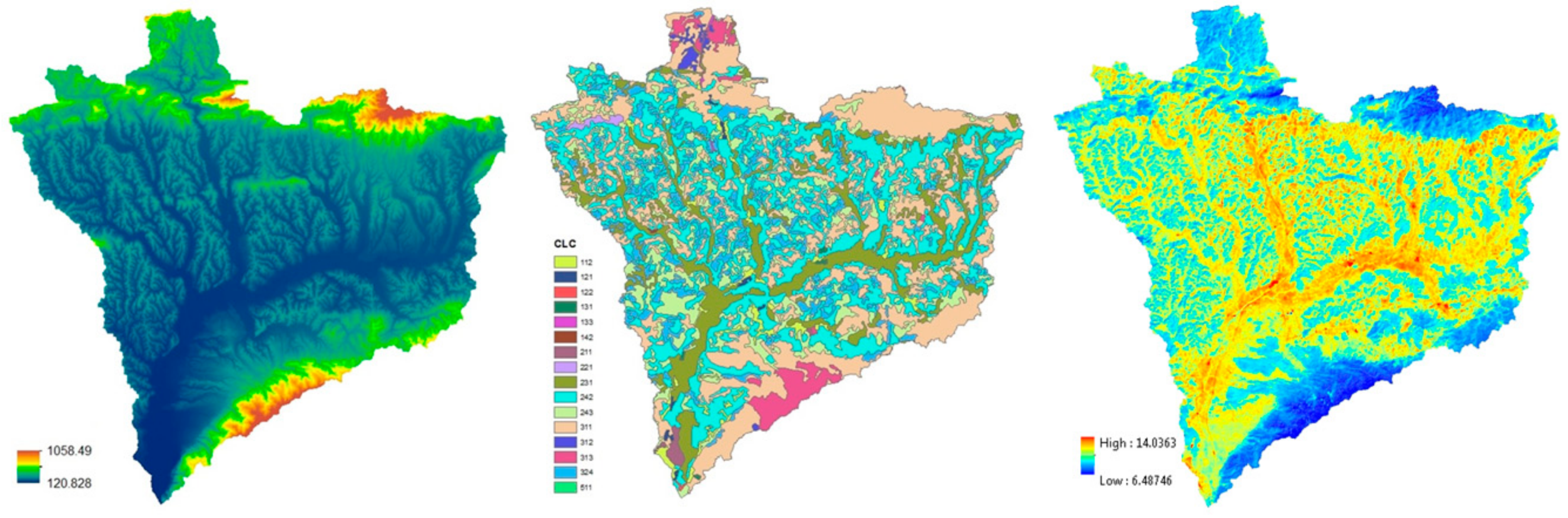
2. Study Area and Data

The Krapina River basin, located in the Northern part of Croatia, is part of the wider Danube River basin (Figure 1). The Krapina River emerges from the Ivanscica hillslopes at app. 1000 m a.s.l. and discharges into the Sava River at app. 130 m a.s.l. (Figure 2). The heart-shaped basin covers an area of 1236 km². Agricultural lands (58%) and forests (40%) cover the majority of the basin (13% are pastures and meadows) and the rest (2%) is divided between urbanised areas, industry and roads, see Figure 2. The climate is typically continental–humid with moderate summers and cold and rainy winters. The air temperature (Figure 2) varies from +30 °C and above in summer periods (June, July, August) to 0 °C and below in the winter months, with recorded extremes of −17.2 °C in December, −20.5 °C in January, −22.0 °C in February and −15.5 °C in March.

The remote sensing dataset included 87 satellite images available for the study area. The images were obtained with Landsat 7 ETM+ (Enhanced Thematic Mapper Plus) from the launch of the satellite in April 1999 until June 2003. Due to the loss of the scan line corrector on board the Landsat 7 satellite, images recorded after June 2003 are not usable [26]. After excluding images acquired during the night, with significant cloud cover or low sun elevation, a set of 26 images, at 30 m resolution, recorded during the period 1999–2003, were used in further analyses.

Lysimeter measurements for the period 1999–2002 were available at two locations around the basin: the agro-ecological station Zagreb–Maksimir (available for the period 1990–1999) and the infiltrometric station Varkom–Varazdin (available for the period 1988–2002) (Figure 1). The meteorological dataset comprised the mean, maximum and minimum daily air temperature (T_avg, T_max, T_min), daily relative air humidity (RH) and daily wind speed (u) during the period 1999–2003 at nine stations in and around the basin (Croatian gauges being Krapina, Pregrada, Puntijarka, Stubicke Toplice, Sv. Ivan Zelina and Slovenian gauges being Bizeljsko, Cerklje ob Krki, Metlika, Slovenske Konjice), see Figure 1. Insolation (n) was available only at the Krapina station.

3. Methodology

3.1. SEBAL ET Estimates

As remote sensing provides easily accessible spatial datasets, ET estimation using satellite imagery is becoming relatively common and is the most efficient technology in use nowadays [3,5,27,28,29]. In the surface energy balance approach [6,14,24], the latent heat flux (λET) is computed as the energy residual of the incoming net surface radiation R_n [W m⁻²], the soil (G) and sensible heat (H) fluxes [W m⁻²] using the following equation:

$$\lambda ET=R_n-G-H$$

(1)

The calculation of incoming radiation and two energy fluxes requires ground-based meteorological measurements and satellite images. The SEBAL approach has been successfully implemented for ET estimates across a variety of climates, soil moisture conditions and vegetation covers [6,10,24,27]. The expected relatively high accuracy of daily, seasonal and annual ET estimates, of 85%, 95% and 96% [30], respectively, are somewhat lower when applied in mountainous areas [31,32]. The advantages of the SEBAL approach for ET estimates include automatic internal calibration within each analysed image (assumptions about the energy balance state are made at the hottest and the coolest pixels in the image) and minimum auxiliary ground-based data [27]. The obtained instantaneous latent heat flux can be converted into daily ET through the evaporative fraction (Λ), which is defined as the ratio between the latent heat flux and the available energy (R_n − G):

$$\mathsf{\Lambda }=\frac{\lambda ET}{R_n-G}$$

(2)

Results obtained in [6,24,33] show that Λ is stable during the day and this assumption is used in further estimation of daily ET from satellite images.

3.2. Obtaining Daily ET by Using Interpolated Evaporative Fraction

The proposed approach is an upgrade of the method proposed for seasonal basin wide ET estimates [6,14,24] making it possible to estimate daily ET in periods with no satellite images available.

The daily ET is estimated by using the interpolated evaporative fraction (Λ_INT) from available satellite images. Λ_INT is derived from several instantaneous Λ rasters as

$${\mathsf{\Lambda }}_{INT}=\frac{1}{N}{\displaystyle \sum }_{i=1}^N{\mathsf{\Lambda }}_{XY}$$

(3)

where Λ_INT and Λ_XY are the interpolated and the instantaneous Λ in cell xy, respectively, and N is the number of instantaneous Λ. The daily ET is obtained by multiplying Λ_INT and PET rasters over the area as:

$$E{T}_{A,XY}={\mathsf{\Lambda }}_{INT}·E{T}_{P,XY}$$

(4)

with ET_A,XY is the obtained daily ET [mm day⁻¹] and ET_P,XY is PET in the corresponding cell, xy (mm day⁻¹). Variations in the proposed approach include the number of interpolated available images and the applied PET method.

To evaluate the required number of satellite images for reliable estimatation of Λ_INT, a total of five sets are tested, comprising 1, 5, 10, 15 and 26 consecutive images. The selected Λ_INT raster is then combined with the PET method to obtain the daily ET estimates. Five standard methods for PET estimates are evaluated by comparing daily ET rasters and SEBAL ET estimates. The Turc, Hargreaves–Samani, Penman–Monteith, Makkink and Priesley–Taylor [12,13] methods are included with the initial spatial interpolation of point input parameters (T_avg, T_min, T_max, RH, u, n).

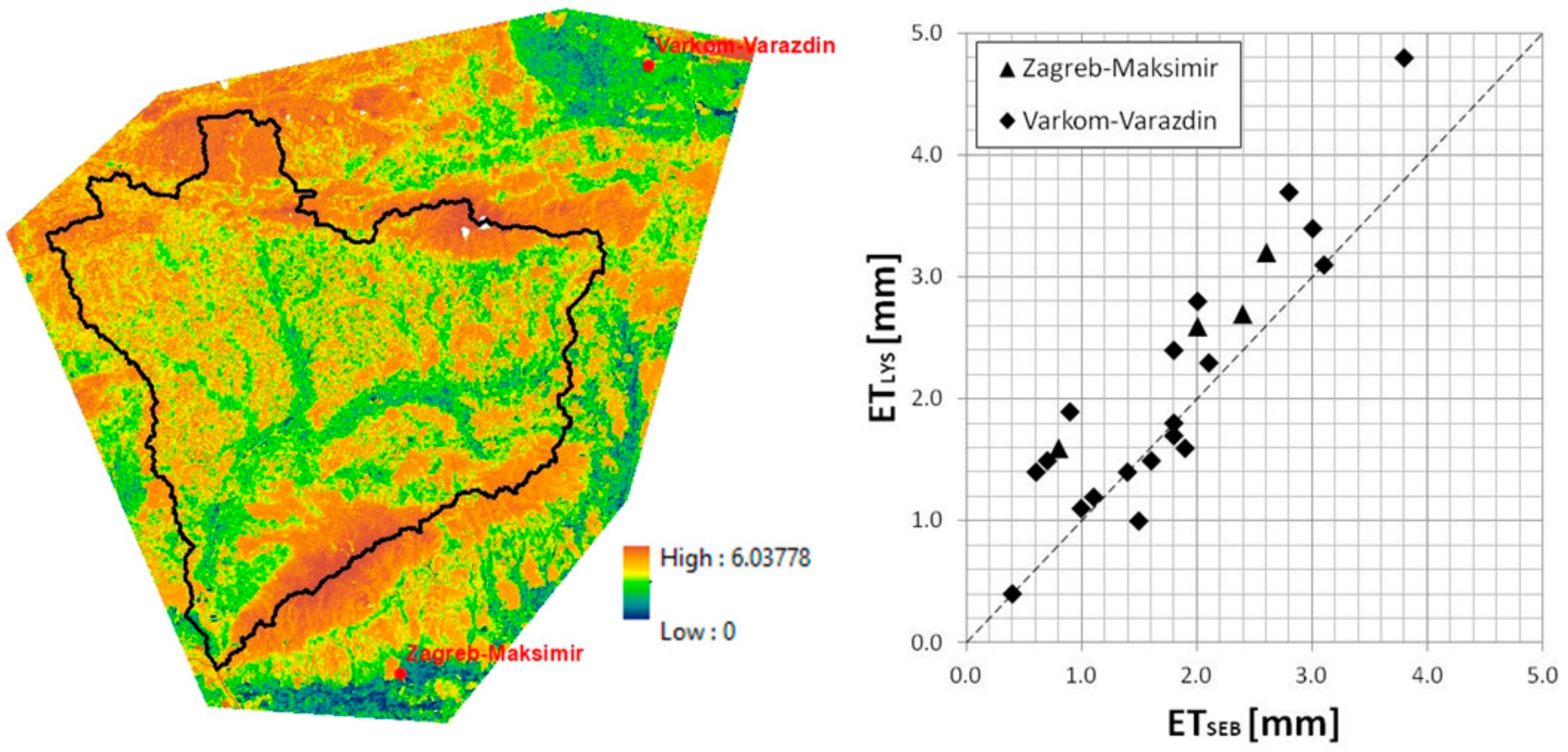
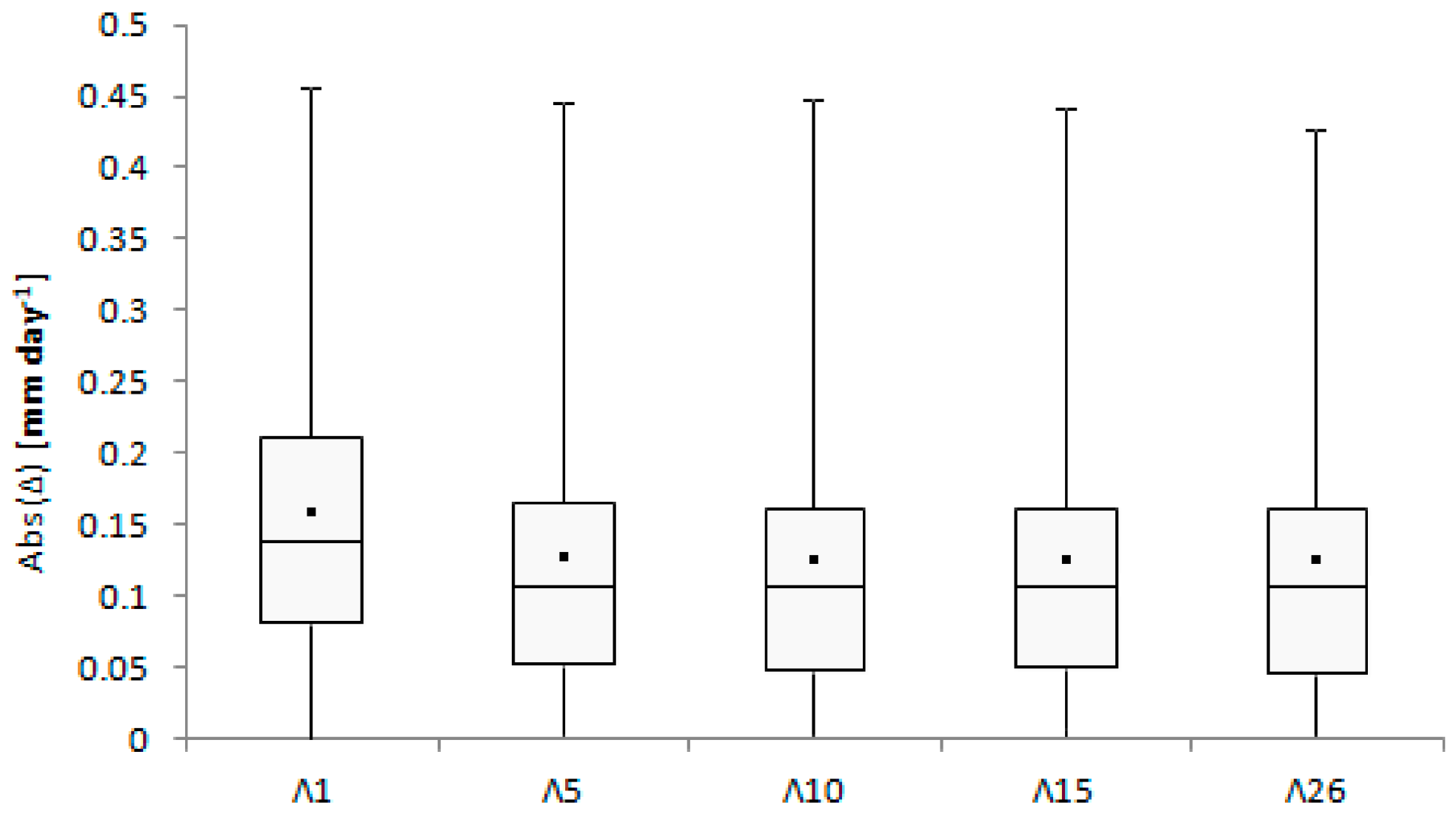
3.3. Validation and Sensitivity Analysis

The reliability of obtained ET estimates and PET methods is evaluated through the analysis of residuals (∆), standard deviations of residuals (σ) and the Nash-Sutcliffe efficiency (NSE) for the SEBAL ET estimates. The residuals (∆) are formed as

$$\Delta =\frac{1}{N}{\displaystyle \sum }_{i=1}^N{\left(E{T}_{XY}-E{T}_{SEB,XY}\right)}_i$$

(5)

where ET_XY is the obtained ET/PET, and ET_SEB,XY is the SEBAL ET in the corresponding cell, xy. The Nash–Sutcliffe efficiency (NSE) determines the relative magnitude of the residual variance:

$$NSE=1-\left[\frac{{{\displaystyle \sum }}_{i=1}^N{\left(E{T}_{SEB,XY}-E{T}_{XY}\right)}^2}{{{\displaystyle \sum }}_{i=1}^N{\left(E{T}_{SEB,XY}-E{T}_{SEB,XY,MEAN}\right)}^2}\right]$$

(6)

where ET_SEB,XY,MEAN is the mean of the SEBAL ET from the observed data.

4. Results

4.1. Measured ET in the Krapina River Basin

Remote sensing allows a definition of spatially distributed basin wide AET, but with one major drawback: the procedure depends on the usability of the input data in terms of the image quality and the availability of the acquired images. The number of usable images covering the Krapina River basin acquired during the analysed period (1999–2003) is only 26.

The results of the SEBAL method (ET_SEB) were compared to the daily ET values (ET_LYS) derived from weekly and decadal measurements at the Varkom–Varazdin (compared for the period 1999–2002) and Zagreb–Maksimir (compared for 1999) gauging stations (Figure 3). Residuals between gauging stations measurements and SEBAL estimates at their locations for the overlapping period (1999–2002) fall within the range of 0.0–1.0 mm and have the following values: average Δ = 0.3 mm, σ = 0.44 mm and NSE = 0.64; this confirms the high reliability of the SEBAL method.

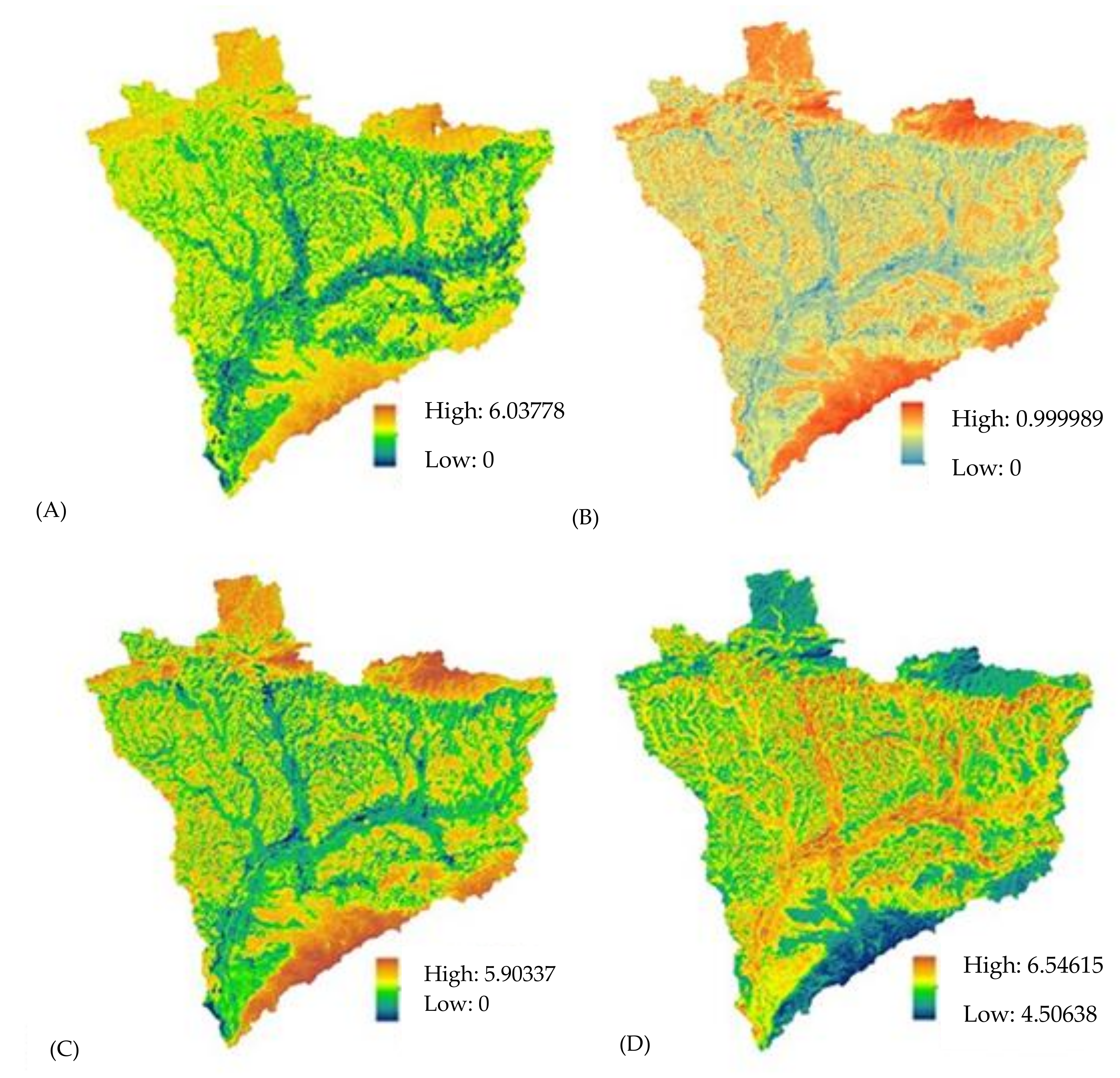
4.2. Evaporative Fraction Variability and Interpolation

The validation and sensitivity analyses regarding variations in Λ_INT depending on the number of Λ used for interpolation, consist of comparing Λ_INT rasters with instantaneous Λ rasters computed for each satellite image, i.e., analysing Δ and σ (

Table 1. Validation of Λ_INT depending on the number of Λ used for interpolation. MAE: Mean absolute errors.

Image No.	Acquisition Date	Λ1		Λ5		Λ10		Λ15		Λ26
		Δ [mm day−1]	σ [mm day−1]	Δ [mm day−1]	σ [mm day−1]	Δ [mm day−1]	σ [mm day−1]	Δ [mm day−1]	σ [mm day−1]	Δ [mm day−1]	σ [mm day−1]
1	6 July 1999	0.03	0.25	0.17	0.14	0.19	0.16	0.18	0.17	0.17	0.16
2	15 July 1999	−0.20	0.19	−0.06	0.10	−0.04	0.11	−0.04	0.12	−0.06	0.11
3	7 August 1999	−0.19	0.21	−0.06	0.10	−0.03	0.13	−0.04	0.13	−0.06	0.13
4	24 September 1999	−0.10	0.18	0.04	0.10	0.06	0.11	0.05	0.11	0.04	0.11
5	18 March 2000	−0.21	0.34	−0.08	0.30	−0.05	0.31	−0.06	0.31	−0.07	0.32
6	28 April 2000	0.14	0.30	0.28	0.31	0.30	0.28	0.30	0.28	0.28	0.27
7	14 May 2000	−0.32	0.18	−0.19	0.15	−0.16	0.11	−0.17	0.11	−0.18	0.11
8	21 May 2000	−0.13	0.20	0.01	0.26	0.04	0.20	0.03	0.20	0.02	0.20
9	6 June 2000	−0.26	0.17	−0.13	0.12	−0.10	0.08	−0.11	0.09	−0.12	0.08
10	15 June 2000	−0.30	0.18	−0.16	0.16	−0.13	0.12	−0.14	0.13	−0.15	0.12
11	2 August 2000	0.00	0.00	0.14	0.18	0.16	0.13	0.15	0.12	0.14	0.12
12	10 September 2000	−0.10	0.16	0.04	0.24	0.06	0.19	0.05	0.18	0.04	0.18
13	6 April 2001	−0.10	0.16	0.04	0.16	0.07	0.13	0.06	0.12	0.04	0.12
14	1 May 2001	−0.03	0.16	0.10	0.17	0.13	0.13	0.12	0.11	0.11	0.12
15	24 May 2001	−0.16	0.16	−0.02	0.18	0.00	0.13	−0.01	0.12	−0.02	0.13
16	25 June 2001	−0.31	0.20	−0.16	0.17	−0.15	0.15	−0.15	0.14	−0.17	0.13
17	12 August 2001	−0.45	0.21	−0.32	0.14	−0.29	0.14	−0.30	0.15	−0.31	0.14
18	8 October 2001	0.04	0.16	0.17	0.12	0.20	0.10	0.19	0.10	0.18	0.09
19	12 June 2002	−0.02	0.21	0.12	0.14	0.15	0.14	0.14	0.15	0.12	0.13
20	21 June 2002	−0.14	0.18	0.00	0.17	0.02	0.14	0.02	0.14	0.00	0.13
21	24 August 2002	−0.09	0.15	0.05	0.17	0.07	0.14	0.06	0.14	0.05	0.13
22	31 August 2002	−0.21	0.16	−0.07	0.14	−0.05	0.12	−0.05	0.12	−0.07	0.10
23	20 March 2003	−0.02	0.18	0.11	0.17	0.14	0.15	0.13	0.14	0.12	0.14
24	27 March 2003	0.29	0.17	0.42	0.15	0.45	0.13	0.44	0.12	0.43	0.12
25	7 May 2003	0.08	0.14	0.21	0.15	0.24	0.11	0.23	0.09	0.22	0.10
26	30 May 2003	−0.15	0.18	−0.01	0.20	0.02	0.15	0.01	0.15	−0.01	0.15
MAE		0.16	0.18	0.14	0.17	0.13	0.15	0.13	0.14	0.13	0.14
Min		−0.45	0.00	−0.32	0.10	−0.29	0.08	−0.30	0.09	−0.31	0.08
Max		0.29	0.34	0.42	0.31	0.45	0.31	0.44	0.31	0.43	0.32

). Analyses include using the following images for interpolation: 1 (the first available completely cloud free satellite image i.e., 2 August 2000), 5 (6 July 1999–18 March 2000), 10 (6 July 1999–15 June 2000), 15 (6 July 1999–24 May 2001) and all 26 acquired Λ rasters (with clouds being extracted from satellite images).

Mean absolute errors (MAE) of Δ for analysed variations range from 0.16 mm for a single Λ to 0.13 mm for the 26 Λ used for interpolation. The mean absolute error for σ is within the interval 0.14–0.18 mm for all variations.

Depending on the number of Λ used for defining the interpolated basin wide Λ_INT, the results indicate that using 5 Λ for interpolation provides satisfactory results, with accuracy not increasing with a further number increase, as shown in Figure 4, in absolute Δ values.

The Λ_INT shown in Figure 5B results from 5 Λ rasters computed using images acquired during the period from 6 July 1999 to 18 March 2000. To evaluate the altitude variability of Λ_INT, it is compared to each instantaneous Λ acquired for the whole basin as well as for altitude classes. The definition of basin altitude class boundaries is based on altitude quantiles: 0–20%, 20–40%, 40–60%, 60–80% and 80–100%.

Validation of Λ_INT consists of analysing Δ and σ (

Table 2. Variability between Λ_INT and instantaneous Λ for altitude classes.

Image No.	Acquisition Date	ETSEB,MEAN [mm day−1]	ΛMEAN [1]	Δ [1]	σ [1]	Δ [1]	σ [1]	Δ [1]	σ [1]	Δ [1]	σ [1]	Δ [1]	σ [1]	Δ [1]	σ [1]
Altitude Class (m a.s.l.)		Basin				68–163		163–195		195–228		228–302		302–1053
1	6 July 1999	2.92	0.35	0.17	0.14	0.07	0.14	0.13	0.16	0.18	0.16	0.2	0.16	0.28	0.13
2	15 July 1999	3.21	0.58	−0.06	0.10	−0.07	0.11	−0.07	0.12	−0.06	0.12	−0.06	0.12	−0.04	0.09
3	7 August 1999	3.75	0.6	−0.06	0.10	−0.12	0.11	−0.08	0.13	−0.05	0.13	−0.05	0.14	0.01	0.11
4	24 September 1999	1.11	0.5	0.04	0.10	0.03	0.11	0.06	0.11	0.06	0.12	0.05	0.11	0.02	0.1
5	18 March 2000	0.87	0.67	−0.08	0.30	0.07	0.32	−0.04	0.35	−0.07	0.33	−0.13	0.32	−0.22	0.2
6	28 April 2000	0.73	0.22	0.28	0.31	0.18	0.3	0.27	0.27	0.3	0.26	0.34	0.23	0.32	0.22
7	14 May 2000	3.75	0.7	−0.19	0.15	−0.23	0.13	−0.18	0.12	−0.16	0.1	−0.16	0.1	−0.15	0.07
8	21 May 2000	2.17	0.46	0.01	0.26	0.04	0.19	0.06	0.21	0.0	0.2	0.01	0.2	−0.06	0.18
9	6 June 2000	3.86	0.66	−0.13	0.12	−0.12	0.09	−0.13	0.09	−0.13	0.08	−0.13	0.08	−0.09	0.06
10	15 June 2000	4.15	0.67	−0.16	0.16	−0.15	0.13	−0.16	0.12	−0.15	0.11	−0.15	0.13	−0.13	0.11
11	2 August 2000	2.6	0.4	0.14	0.18	0.19	0.12	0.15	0.13	0.13	0.12	0.13	0.12	0.09	0.09
12	10 September 2000	1.77	0.5	0.04	0.24	0.14	0.17	0.05	0.18	0.01	0.17	0.02	0.19	−0.04	0.18
13	6 April 2001	1.4	0.5	0.04	0.16	0.09	0.12	0.05	0.12	0.04	0.12	0.02	0.12	0.0	0.13
14	1 May 2001	2.15	0.43	0.10	0.17	0.06	0.15	0.12	0.13	0.12	0.12	0.12	0.11	0.11	0.08
15	24 May 2001	3.11	0.55	−0.02	0.18	−0.07	0.15	0.0	0.13	0.0	0.12	0.01	0.12	−0.04	0.08
16	25 June 2001	3.82	0.67	−0.16	0.17	−0.24	0.18	−0.19	0.13	−0.18	0.11	−0.15	0.1	−0.13	0.09
17	12 August 2001	4.06	0.83	−0.32	0.14	−0.3	0.15	−0.33	0.14	−0.32	0.14	−0.33	0.14	−0.27	0.09
18	8 October 2001	0.77	0.35	0.17	0.12	0.17	0.1	0.17	0.1	0.19	0.09	0.19	0.09	0.18	0.08
19	12 June 2002	2.45	0.41	0.12	0.14	0.11	0.13	0.13	0.13	0.14	0.13	0.12	0.14	0.08	0.13
20	21 June 2002	3.41	0.52	0.00	0.17	0.02	0.16	−0.01	0.13	−0.01	0.12	0.0	0.13	0.01	0.1
21	24 August 2002	1.86	0.48	0.05	0.17	0.12	0.14	0.06	0.13	0.03	0.12	0.01	0.13	0.01	0.11
22	31 August 2002	2.48	0.58	−0.07	0.14	−0.04	0.16	−0.08	0.1	−0.09	0.09	−0.08	0.08	−0.07	0.06
23	20 March 2003	0.95	0.47	0.11	0.17	0.11	0.15	0.1	0.15	0.12	0.14	0.14	0.14	0.12	0.14
24	27 March 2003	0.52	0.12	0.42	0.15	0.39	0.09	0.42	0.11	0.44	0.11	0.45	0.11	0.41	0.16
25	7 May 2003	2.37	0.32	0.21	0.15	0.22	0.12	0.23	0.11	0.22	0.1	0.22	0.09	0.2	0.07
26	30 March 2003	3.37	0.53	−0.01	0.20	−0.02	0.18	0.02	0.15	0.0	0.13	0.0	0.14	−0.05	0.12
Avg		2.45	0.5	0.02	0.17	0.02	0.15	0.03	0.14	0.03	0.14	0.03	0.14	0.02	0.11
Min		0.52	0.12	−0.32	0.10	−0.3	0.09	−0.33	0.09	−0.32	0.08	−0.33	0.08	−0.27	0.06
Max		4.15	0.83	0.42	0.31	0.39	0.32	0.42	0.35	0.44	0.33	0.45	0.32	0.41	0.22

) for each event. The average Δ for the whole basin is 0.02 (2%) with an average σ of 0.17 (17%), with almost constant values for all altitude classes (average Δ range from 0.02 to 0.03, i.e., 2% to 3%, with an average σ within the interval 0.11–0.15, i.e., 11–15%). Lower average Δ values (Table 2) than MAE Δ values (Table 1) for the whole basin indicate the self-cancelling characteristic of summed Λ residuals.

4.3. Daily ET Modelling Based on PET Variation

Five daily ET rasters for each observed event (date of image acquisition) are modelled by multiplying Λ_INT with various PET rasters (4) using the Turc (T), Hargreaves–Samani (HS), Penman–Monteith (PM), Makkink (M) and Priestley–Taylor (PT) methods. Results are compared to the SEBAL ET.

Validation and sensitivity analyses regarding variations in the proposed approach depending on the chosen PET method consist of comparing resulting daily ET rasters with the SEBAL ET, i.e., analysing Δ, σ and NSE (

Table 3. AET raster residuals (Δ), standard deviation of the residuals (σ) and the Nash–Sutcliffe efficiency (NSE) for PET variations.

Image No.	Acquisition Date	Δ [mm Day−1]					σ [mm Day−1]					NSE
		T	HS	PM	M	PT	T	HS	PM	M	PT	T	HS	PM	M	PT
1 *	6 July 1999	0.39	0.28	1.08	0.38	0.58	1.08	0.98	1.22	1.08	1.09	0.3	0.11	−0.8	−0.03	0.11
2 *	15 July 1999	−0.25	−0.72	−0.61	−0.17	0	0.6	0.55	0.57	0.62	0.63	0.1	0.54	0.24	0.56	0.53
3 *	7 August 1999	−0.54	−0.96	−0.46	−0.55	−0.42	0.74	0.61	0.76	0.74	0.75	−0.42	0.05	0.11	0.17	0.07
4 *	24 September 1999	0.83	0.41	0.29	0.81	0.51	0.31	0.29	0.26	0.31	0.27	0.07	−1.82	0.42	−0.24	−1.94
5 *	18 March 2000	−0.97	−0.16	−0.12	0.17	−0.07	0.85	0.51	0.5	0.47	0.49	0.15	0.26	0.22	0.29	−3.88
6	28 April 2000	1.24	1.34	1.11	1.23	1.34	0.79	0.79	0.78	0.79	0.8	−2.61	−2.2	−1.74	−2.61	−2.23
7	14 May 2000	−1.01	−1.17	−1.23	−0.83	−0.89	0.6	0.62	0.59	0.61	0.61	−0.76	−0.08	−0.87	−0.17	−0.38
8	21 May 2000	−0.11	0.16	−0.22	0.12	0.19	0.92	0.93	0.91	0.85	0.84	0.57	0.64	0.57	0.63	0.58
9	6 June 2000	−0.66	−0.76	−0.99	−0.63	−0.41	0.47	0.44	0.44	0.49	0.52	0.11	0.28	−0.33	0.49	0.24
10	15 June 2000	−0.79	−1.24	−1.16	−0.75	−0.51	0.77	0.76	0.75	0.78	0.8	−0.41	0.22	−0.26	0.39	0.18
11	2 August 2000	0.63	0.3	0.36	0.66	0.71	0.85	1.04	0.87	0.84	0.87	0.55	0.57	0.66	0.52	0.57
12	10 September 2000	0.2	0	−0.14	0.26	−0.05	0.68	0.8	0.74	0.65	0.72	0.5	0.61	0.55	0.59	0.61
13	6 April 2001	−0.1	0	−0.11	0.2	0.02	0.43	0.42	0.39	0.36	0.38	0.59	0.59	0.6	0.65	0.54
14	1 May 2001	0.44	0.39	0.21	0.46	0.47	0.61	0.68	0.62	0.6	0.61	0.48	0.51	0.63	0.49	0.52
15	24 May 2001	−0.16	−0.52	−0.48	−0.01	−0.03	0.74	0.83	0.78	0.72	0.72	0.48	0.72	0.55	0.72	0.69
16	25 June 2001	−0.59	−1.02	−0.91	−0.53	−0.33	0.73	0.67	0.69	0.75	0.77	−0.48	0.16	−0.31	0.29	0.12
17	12 August 2001	−1.52	−2.1	−1.68	−1.38	−1.47	0.59	0.52	0.55	0.63	0.62	−6.14	−2.52	−3.78	−2−.91	−3.06
18	8 October 2001	0.72	0.37	0.22	0.67	0.31	0.23	0.22	0.2	0.22	0.2	−0.18	−2.03	0.43	0.14	−2.55
19	12 June 2002	0.94	0.41	0.76	1	0.87	0.84	0.81	0.81	0.84	0.87	0.35	−0.34	0.05	−0.78	−0.23
20	21 June 2002	0.01	−0.14	−0.15	0	0.38	0.79	0.87	0.81	0.79	0.79	0.62	0.69	0.67	0.62	0.69
21	24 August 2002	0.47	0.04	−0.01	0.46	0.53	0.48	0.54	0.52	0.48	0.48	0.6	0.39	0.62	0.29	0.37
22	31 August 2002	−0.27	−0.76	−0.56	−0.29	−0.34	0.43	0.44	0.43	0.43	0.43	−0.08	0.63	0.3	0.58	0.64
23	20 March 2003	−0.07	0.16	0.06	0.36	0.05	0.41	0.4	0.35	0.33	0.35	0.26	0.03	0.49	0.5	0.3
24	27 March 2003	1.03	0.97	1.59	1.19	0.77	0.52	0.58	0.5	0.5	0.53	−1.16	−1.81	−3.64	−0.49	−1.27
25	7 May 2003	0.78	0.85	1.05	0.78	0.67	0.82	0.99	0.79	0.81	0.85	0.29	0.47	0.28	0.51	0.46
26	30 May 2003	−0.19	−0.99	−0.54	−0.14	0.02	0.96	1.06	1.01	0.95	0.94	0.14	0.62	0.47	0.64	0.61
Avg (only *)		−0.11	−0.23	0.04	0.13	0.12	0.72	0.59	0.66	0.64	0.65	0.04	−0.17	0.04	0.15	−1.02
Min (only *)		−0.97	−0.96	−0.61	−0.55	−0.42	0.31	0.29	0.26	0.31	0.27	−0.42	−1.82	−0.80	−0.24	−3.88
Max (only *)		0.83	0.41	1.08	0.81	0.58	1.08	0.98	1.22	1.08	1.09	0.30	0.54	0.42	0.56	0.53
Avg		0.02	−0.19	−0.10	0.13	0.11	0.66	0.67	0.65	0.64	0.65	−0.23	−0.10	−0.15	0.07	−0.30
Min		−1.52	−2.10	−1.68	−1.38	−1.47	0.23	0.22	0.20	0.22	0.20	−6.14	−2.52	−3.78	−2.91	−3.88
Max		1.24	1.34	1.59	1.23	1.34	1.08	1.06	1.22	1.08	1.09	0.62	0.72	0.67	0.72	0.69

* used for defining Λ_INT; PET variations: T—Turc, HS—Hargreaves-Samani, PM—Penman-Monteith, M—Makkink and PT—Priestley-Taylor method.

) for each event. The average Δ for analysed variations ranges from −0.19 mm for HS to 0.13 mm for the M variation. The average σ is within the interval, 0.64–0.67 mm, for all variations. The average NSE ranges from −0.30 for PT to 0.07 for the M variation.

Based on the chosen PET method for modelling daily ET, all analysed variations provide satisfactory results, with the Makkink variation being considered the most appropriate. Spatial distributions of SEBAL ET and daily ET rasters, as exemplified with the event on 6th June 2000 (Figure 5A,C), experience the same spatial pattern (ET increases with the altitude, reaching its maximum in areas covered with healthier and dense vegetation).

4.4. Validation of Proposed Concept

The validation of the application of Λ_INT, interpolated using five instantaneous Λ rasters, for estimating daily ET outside the Λ interpolation period (6 July 1999–18 March 2000), shows no significant differences between the accuracy of results outside the Λ interpolation period (

Table 4. Validation of proposed concept: raster residuals (Δ), standard deviations of the residuals (σ) and Nash–Sutcliffe efficiency (NSE).

Image No.	Acquisition Date	Δ [mm Day−1]	σ [mm Day−1]	NSE
6	28 April 2000	1.23	0.79	−2.61
7	14 May 2000	−0.83	0.61	−0.17
8	21 May 2000	0.12	0.85	0.63
9	6 June 2000	−0.63	0.49	0.49
10	15 June 2000	−0.75	0.78	0.39
11	2 August 2000	0.66	0.84	0.52
12	10 September 2000	0.26	0.65	0.59
13	6 April 2001	0.2	0.36	0.65
14	1 May 2001	0.46	0.6	0.49
15	24 May 2001	−0.01	0.72	0.72
16	25 June 2001	−0.53	0.75	0.29
17	12 August 2001	−1.38	0.63	−2.91
18	8 October 2001	0.67	0.22	0.14
19	12 June 2002	1	0.84	−0.78
20	21 June 2002	0	0.79	0.62
21	24 August 2002	0.46	0.48	0.29
22	31 August 2002	−0.29	0.43	0.58
23	20 March 2003	0.36	0.33	0.5
24	27 March 2003	1.19	0.5	−0.49
25	7 May 2003	0.78	0.81	0.51
26	30 May 2003	−0.14	0.95	0.64
Avg		0.13	0.64	0.05
Min		−1.38	0.22	−2.91
Max		1.23	0.98	0.72

). The observed Δ, σ and NSE regarding events during the Λ interpolation period (Table 3, Makkink variation: Δ = 0.13 mm day⁻¹, σ = 0.64 mm day⁻¹ and NSE = −0.15) and events outside the Λ interpolation period using previously defined Λ_INT for daily ET estimates (21 images) are almost the same (Table 4: Δ = 0.13 mm day⁻¹, σ = 0.64 mm day⁻¹ and NSE = 0.05).

4.5. Standard PET Methods

Another simple approach for basin wide ET estimation, frequently used when no satellite images are available, is spatial interpolation of point PET estimates, usually using one of the standard methods: Turc (T), Hargreaves–Samani (HS), Penman–Monteith (PM), Makkink (M) or Priestley–Taylor (PT) method.

Validation and sensitivity analyses regarding PET methods consist of comparing the results from PET with SEBAL ET, i.e., analysing Δ, σ and NSE (

Table 5. Raster residuals (Δ), standard deviations of the residuals (σ) and Nash–Sutcliffe efficiency (NSE) for PET methods.

Image No.	Acquisition Date	Δ [mm Day−1]					σ [mm Day−1]					NSE
		T	HS	PM	M	PT	T	HS	PM	M	PT	T	HS	PM	M	PT
1	6 July 1999	3.22	3.16	4.47	3.19	3.58	1.10	1.40	1.06	1.09	1.13	−7.00	−6.62	−13.11	−8.42	−6.76
2	15 July 1999	2.30	1.49	1.61	2.42	2.77	0.91	1.08	0.86	0.86	0.90	−2.65	−6.14	−2.62	−8.16	−5.61
3	7 August 1999	2.17	1.49	2.28	2.15	2.39	0.80	1.03	0.79	0.78	0.80	−2.63	−4.74	−5.40	−5.98	−4.88
4	24 September 1999	2.49	1.77	1.50	2.45	1.89	0.52	0.71	0.55	0.50	0.50	−12.37	−21.92	−8.41	−12.99	−22.86
5	18 March 2000	−0.88	0.48	0.53	1.09	0.62	1.07	0.70	0.66	0.65	0.63	−1.12	−3.76	−1.10	−1.30	−4.59
6	28 April 2000	3.03	3.28	2.80	2.99	3.19	0.93	1.08	1.00	0.91	0.91	−16.68	−13.53	−12.14	−15.30	−13.88
7	14 May 2000	1.36	1.14	0.94	1.67	1.57	1.02	1.25	0.98	0.97	0.99	−1.88	−2.72	−0.85	−2.45	−1.91
8	21 May 2000	1.75	2.33	1.51	2.18	2.32	1.46	1.62	1.38	1.40	1.41	−2.92	−2.25	−1.04	−2.58	−1.53
9	6 June 2000	2.05	1.95	1.48	2.11	2.51	0.94	1.19	1.01	0.90	0.91	−4.91	−4.96	−2.62	−7.03	−4.78
10	15 June 2000	2.20	1.47	1.54	2.27	2.71	1.15	1.47	1.23	1.12	1.12	−1.87	−3.26	−1.60	−4.70	−3.10
11	2 August 2000	3.39	2.87	2.85	3.42	3.55	1.66	1.98	1.57	1.63	1.74	−3.59	−4.41	−2.99	−4.91	−4.37
12	10 September 2000	1.96	1.64	1.31	2.07	1.48	1.19	1.38	1.17	1.16	1.16	−2.60	−3.41	−1.41	−1.77	−3.12
13	6 April 2001	1.07	1.26	0.99	1.62	1.28	0.80	0.81	0.68	0.70	0.71	−4.23	−6.18	−2.36	−3.95	−3.12
14	1 May 2001	2.65	2.66	2.22	2.67	2.71	1.08	1.38	1.08	1.05	1.07	−6.61	−5.95	−4.16	−6.17	−5.93
15	24 May 2001	2.35	1.76	1.77	2.62	2.70	1.38	1.56	1.39	1.32	1.32	−1.97	−3.63	−1.72	−3.85	−3.00
16	25 June 2001	2.35	1.61	1.75	2.45	2.84	1.00	1.20	1.03	0.97	0.99	−3.00	−5.90	−3.11	−7.94	−5.47
17	12 August 2001	0.68	−0.36	0.41	0.92	0.74	0.77	0.82	0.85	0.71	0.70	−0.23	−1.08	−0.38	−0.60	−0.63
18	8 October 2001	2.00	1.40	1.08	1.89	1.24	0.42	0.56	0.42	0.40	0.39	−12.90	−21.64	−7.19	−9.34	−24.49
19	12 June 2002	3.94	3.06	3.64	4.05	4.50	1.15	1.44	1.26	1.12	1.13	−7.86	−12.64	−10.50	−15.66	−12.02
20	21 June 2002	2.96	2.81	2.70	2.93	3.67	1.41	1.81	1.50	1.39	1.42	−4.46	−4.15	−3.66	−6.56	−4.25
21	24 August 2002	2.53	1.78	1.63	2.49	2.64	0.91	1.05	0.97	0.88	0.87	−4.79	−8.50	−3.89	−9.47	−8.83
22	31 August 2002	1.61	0.72	1.10	1.58	1.48	0.78	0.81	0.82	0.76	0.76	−0.62	−3.24	−1.60	−2.85	−3.44
23	20 March 2003	0.71	1.18	0.93	1.50	0.91	0.67	0.74	0.56	0.56	0.55	−6.76	−9.18	−3.74	−3.52	−2.81
24	27 March 2003	2.36	2.29	3.35	2.64	1.87	0.81	0.95	0.71	0.77	0.78	−9.29	−11.67	−18.59	−5.91	−9.49
25	7 May 2003	3.47	3.75	3.96	3.46	3.27	1.56	2.06	1.57	1.53	1.62	−6.57	−4.94	−6.52	−4.53	−5.00
26	30 May 2003	2.63	1.15	2.01	2.71	2.04	1.57	1.63	1.65	1.53	1.53	−0.61	−2.91	−1.72	−3.67	−2.79
Avg		2.17	1.85	1.94	2.37	2.33	1.04	1.22	1.03	0.99	1.00	−5.00	−6.90	−4.71	−6.14	−6.49
Min		−0.88	−0.36	0.41	0.92	0.62	0.42	0.56	0.42	0.40	0.39	−16.68	−21.92	−18.59	−15.66	−24.49
Max		3.94	3.75	4.47	4.05	4.50	1.66	2.06	1.65	1.63	1.74	−0.23	−1.08	−0.38	−0.60	−0.63

T—Turc, HS—Hargreaves-Samani, PM—Penman-Monteith, M—Makkink and PT—Priestley-Taylor method.

) for each event. For PET, the average Δ ranges from 1.85 mm for HS to 2.37 mm for M method. The average σ ranges from 0.99 mm to 1.22 mm and the average NSE ranges from −4.71 for PM to −6.90 for the HS method.

Based on the analysis for all 26 events, the Penman–Monteith method is the most appropriate PET method (Δ = 1.94 mm day⁻¹, σ = 1.03 mm day⁻¹ and NSE = −4.71). Keeping in mind the results of the numerous studies and Food and Agriculture Organization recommendations, the Penman–Monteith method is recommended for spatially describing basin wide PET when the proposed concept cannot be applied.

The cell-based comparison of the daily ET and PET rasters with the SEBAL ET reveals the different spatial dynamics of the resulting ET depending on the method used (Figure 6). In general, PET decreases as SEBAL ET increases, while ET based on the proposed approach experiences the same spatial behaviour as SEBAL ET.

5. Discussion

Remote sensing data greatly increases the accuracy of the estimation of basin wide ET, which is the most significant water balance component and the one most difficult to evaluate, especially in regard to various spatio–temporal scales. The SEBAL method was used for obtaining spatially distributed basin wide ET values that were confirmed using data from two lysimeters (measured during period 1999–2002 with Δ = 0.3 mm, σ = 0.44 mm and NSE = 0.64). With such high accuracy and keeping in mind that the SEBAL method produces spatially justified indirectly measured ET values, the results were evaluated as being suitable to use for validating the results of the ET estimates.

The major drawback of remote sensing ET estimates is the fact that they can be implemented only in periods with available satellite images. An attempt to estimate daily ET for periods without input satellite images was presented, where basin wide daily ET is obtained by combining interpolated Λ using available satellite images and standard PET methods on meteorological stations. The relatively low temporal variability of Λ in the Krapina River basin makes it possible to use interpolated Λ for modelling basin wide daily ET. The analyses showed that a total of five images can provide a reliable estimate of interpolated Λ and thus represent specific characteristics of a basin. The low temporal variability of Λ in this specific basin could be linked to its particular characteristics, with the climate being typically continental–humid, the basin being, to a large extent, covered with forest and keeping in mind that no extensive agricultural production is present. A relatively low temporal variability in Λ may be expected in basins in tropical and humid climates and especially in those covered with forests [34]. A relatively high variability in Λ may be expected in basins in temperate and semi-arid climates, especially in combination with cropland and grassland cover [34,35]. The temporal variability of Λ increases in conditions when the ET is strongly influenced by the variability of soil moisture and water availability in the root zone, which will decrease the efficiency of the proposed method in such basins.

Considering the choice of PET method for daily ET estimates, the Makkink variation provided the best results (Δ = 0.13 mm, σ = 0.64 mm and NSE = 0.07), experiencing slightly better performance than other analyzed variations. The similarity of obtained ET to the SEBAL ET estimates indicates the relatively high accuracy of the proposed concept, with successful validation of the definition of dependency based on only five events for a further 21 events. Further, in regard to seasons, no major difference in residual Δ values was determined. When evaluated in comparison to absolute ET values, the best results are provided in summer months, when absolute ET values are the highest (Figure 7), with cumulative Δ values acting in a self-cancelling manner.

Minimum remote sensing and the ground based inputs required by the proposed concept make it possible to apply for a basin wide estimate of daily ET in data scarce regions during periods with no satellite images available. Taking this into consideration, our results were compared to standard PET methods as another simple approach for basin wide ET estimation. The similarity of standard PET methods (Penman–Monteith providing the best estimates) to the SEBAL ET estimates (Δ = 1.94 mm day⁻¹, σ = 1.03 mm day⁻¹ and NSE = −4.71) indicates much lower accuracy. As opposed to presented concept, the major differences in residual Δ values for PET methods are evident in summer months when the absolute PET values are also the highest (Figure 7). These values are expected, as PET represents the atmospheric water demand, regardless of surface characteristics; hence, it is expected to experience a different spatial pattern in comparison with the AET that takes into consideration numerous factors influencing the process, including the surface characteristics (vegetation cover, thermal characteristics of the surface, etc.).

As exemplified for the event on 6th July 2000 in Figure 5A,C,D, spatial distributions of PET, compared to SEBAL ET and ET based on proposed approach, are evidently different in terms of minimum/maximum values. Higher altitudes in the basin are covered with dense and healthy forest and have lower air and surface temperatures; thus, they experience higher AET but lower PET. Lower altitudes and densely populated and largely urbanized areas experience significantly lower AET but higher PET. When compared to the spatial distribution of the air temperature (Figure 2), one of the major driving factors influencing ET, it is evident that PET follows the same pattern, as expected. On the other hand, vegetation has a great influence on AET; dense and healthy vegetation cover (Figure 2) contributes to the increase in AET but has no effect on the spatial distribution of PET.

6. Conclusions

This paper investigated how “historical” remote sensing datasets may be used for basin wide ET estimation in periods when no satellite images are available. The proposed method was developed around the interpolated evaporative fractions from several instantaneous satellite images which were combined with the standard PET methods on meteorological stations. The daily ET values were compared to the SEBAL ET estimates and with SEBAL estimates initially validated with the lysimeter data. The basin wide ET estimates were also investigated by using spatial interpolation of point PET estimates, together with an adequate number of satellite images for a reliable estimate of the interpolated evaporative fraction. The Penman–Monteith is the preferred method for the basin wide ET estimates when applying the spatial interpolation of point estimates. For ET estimates in periods with no satellite images available, the results suggest application of the Makking variation in combination with five interpolated evaporative fractions. The proposed concept’s relatively high accuracy is evident from the low discrepancy between obtained ET and the SEBAL ET estimates (Δ = 0.13 mm day⁻¹, σ = 0.64 mm day⁻¹, NSE = 0.07). The discrepancy between the Penman–Monteith interpolated ET estimates to the SEBAL ET estimates was significantly higher (Δ = 1.94 mm day⁻¹, σ = 1.03 mm day⁻¹, NSE = −4.71) than for proposed concept. In the case of the Krapina River basin, it was shown that that the addition of an interpolated evaporative fraction from “historical” satellite images may significantly improve basin wide ET estimates in periods with no satellite images available. The physical parameters derived from the optical and the thermal infrared satellite imagery enable physically valid ET estimates and realistic spatial variability. As the presented concept uses a globally available archive of Landsat images, the suggested approach may be used for basin wide estimates of daily ET in data scarce regions and in periods with no satellite images available. The assumption of a relatively low temporal variability of evaporative fractions limits the application of the proposed concept to regions with significant amounts of water (humid and tropical climate). The application of the described method in regions with insufficient water should be conducted with due care and only after prior confirmation of the low temporal variability of evaporative fraction.

References

- UN-Water. Managing Water under Uncertainty and Risk; Report 4; The United Nations World Water Development: Paris, France, 2012. [Google Scholar]
- European Parliament. Policy Department, Economic and Scientific Policy, Water Scarcity and Droughts; European Parliament’s Committee on the Environment, Public Health and Food Safety: London, UK, 2008. [Google Scholar]
- Senay, G.B.; Leake, S.; Nagler, P.L.; Artan, G.; Dickinson, J.; Cordova, J.T.; Glenn, E.P. Estimating basin scale evapotranspiration (ET) by water balance and remote sensing methods. Hydrol. Process. 2011, 25, 4037–4049. [Google Scholar] [CrossRef]
- Zhang, K.; Kimball, J.S.; Running, S.W. A review of remote sensing based actual evapotranspiration estimation. WIREs Water 2016. [Google Scholar] [CrossRef]
- Cristobal, J.; Poyatos, R.; Ninyerola, M.; Llorens, P.; Pons, X. Combining remote sensing and GIS climate modelling to estimate daily forest evapotranspiration in a Mediterranean mountain area. Hydrol. Earth Syst. Sci. 2011, 15, 1563–1575. [Google Scholar] [CrossRef]
- Bastiaanssen, W.G.M.; Menenti, M.; Feddes, R.A.; Holtslag, A.A.M. A remote sensing surface balance algorithm for land (SEBAL). J. Hydrol. 1998, 212–213, 198–212. [Google Scholar] [CrossRef]
- Su, Z. The Surface Energy Balance System (SEBS) for estimation of turbulent heat fluxes. Hydrol. Earth Syst. Sci. 2002, 6, 85–99. [Google Scholar] [CrossRef]
- Gamage, N.; Smakhtin, V.; Perera, B.J.C. Estimation of Actual Evapotranspiration using Remote Sensing data. In Proceedings of the 19th International Congress on Modelling and Simulation, Perth, Australia, 12–16 December 2011; pp. 3356–3362. [Google Scholar]
- Samain, B.; Simons, G.W.H.; Voogt, M.P.; Defloor, W.; Bink, N.-J.; Pauwels, V.R.N. Consistency between hydrological model, large aperture scintillometer and remote sensing based evapotranspiration estimates for a heterogeneous catchment. Hydrol. Earth Syst. Sci. 2012, 16, 2095–2107. [Google Scholar] [CrossRef]
- Horvat, B. Spatial dynamics of actual daily evapotranspiration. Gradjevinar 2013, 65, 693–705. [Google Scholar]
- Zhang, L.; Potter, N.; Hickel, K.; Zhang, Y.; Shao, Q. Water balance modeling over variable time scales based on the Budyko framework—Model development and testing. J. Hydrol. 2008, 360, 117–131. [Google Scholar] [CrossRef]
- Xu, C.-Y.; Chen, D. Comparison of seven models for estimation of evapotranspiration and groundwater recharge using lysimeter measurement data in Germany. Hydrol. Process. 2005, 19, 3717–3734. [Google Scholar] [CrossRef]
- Douglas, E.M.; Jacobs, J.M.; Sumner, D.M.; Ray, R.L. A comparison of models for estimating potential evapotranspiration for Florida land cover types. J. Hydrol. 2009, 373, 366–376. [Google Scholar] [CrossRef]
- Allen, R.G.; Tasumi, M.; Trezza, R. Satellite-based energy balance for mapping evapotranspiration with internalized calibration (METRIC)-Model. J. Irrig. Drain. Eng. 2007, 133, 395–406. [Google Scholar] [CrossRef]
- Kustas, W.P.; Norman, J.M. A two-source energy balance approach using directional radiometric temperature observations for sparse canopy covered surfaces. Agron. J. 2000, 92, 847–854. [Google Scholar] [CrossRef]
- Roerink, G.J.; Su, Z.; Menenti, M. S-SEBI: A simple remote sensing algorithm to estimate the surface energy balance. Phys. Chem. Earth 2000, 25, 147–157. [Google Scholar] [CrossRef]
- Sanchez, J.M.; Kustas, W.P.; Caselles, V.; Anderson, M.C. Modelling surface energy fluxes over maize using a two-source patch model and radiometric soil and canopy temperature observations. Remote Sens. Environ. 2008, 112, 1130–1143. [Google Scholar] [CrossRef]
- Bhattarai, N.; Quackenbush, L.J.; Dougherty, M.; Marzen, L.J. A simple Landsat–MODIS fusion approach for monitoring seasonal evapotranspiration at 30 m spatial resolution. Int. J. Remote Sens. 2014, 36, 115–143. [Google Scholar] [CrossRef]
- Semmens, K.A.; Anderson, M.C.; Kustas, W.P.; Gao, F.; Alfieri, J.G.; McKee, L.; Prueger, J.H.; Hain, C.R.; Cammalleri, C.; Yang, Y.; et al. Monitoring daily evapotranspiration over two California vineyards using Landsat 8 in a multi-sensor data fusion approach. Remote Sens. Environ. 2015. [Google Scholar] [CrossRef]
- Schuurmans, J.M.; Troch, P.A.; Veldhuizen, A.A.; Bastiaanssen, W.G.M.; Bierkens, M.F.P. Assimilation of remotely sensed latent heat flux in a distributed hydrological model. Adv. Water Resour. 2003, 26, 151–159. [Google Scholar] [CrossRef]
- Neale, C.M.U.; Geli, H.M.E.; Kustas, W.P.; Alfieri, J.G.; Gowda, P.H.; Evett, S.R.; Prueger, J.H.; Hipps, L.E.; Dulaney, W.P.; Chávez, J.L.; et al. Soil water content estimation using a remote sensing based hybrid evapotranspiration modeling approach. Adv. Water Resour. 2012, 50, 152–161. [Google Scholar] [CrossRef]
- Parr, D.; Wang, G. Integrating Remote Sensing Data on Evapotranspiration and Leaf Area Index with Hydrological Modeling: Impacts on Model Performance and Future Predictions. J. Hydrometeorol. 2015, 16, 2086–2100. [Google Scholar] [CrossRef]
- Campos, I.; González-Piqueras, J.; Carrara, A.; Villodre, J.; Calera, A. Estimation of total available water in the soil layer by integrating actual evapotranspiration data in a remote sensing-driven soil water balance. J. Hydrol. 2016, 534, 427–439. [Google Scholar] [CrossRef]
- SEBAL (Surface Energy Balance Algorithms for Land). Advanced Training and Users Manual, Version 1.0; Waters Consulting: Nelson, BC, Canada; University of Idaho: Kimberly, Idaho; WaterWatch Inc.: Wageningen, The Netherlands, 2002. [Google Scholar]
- Singh, R.K.; Liu, S.; Tieszen, L.L.; Suyker, A.E.; Verma, S.B. Estimating seasonal evapotranspiration from temporal satellite images. Irrig. Sci. 2012, 30, 303–313. [Google Scholar] [CrossRef]
- Chen, J.; Zhu, X.; Vogelmann, J.E.; Gao, F.; Jin, S. A simple and effective method for filling gaps in Landsat ETM+ SLC-off images. Remote Sens. Environ. 2011, 115, 1053–1064. [Google Scholar] [CrossRef]
- Liou, Y.-A.; Kar, S.K. Evapotranspiration Estimation with Remote Sensing and Various Surface Energy Balance Algorithms-A Review. Energies 2014, 7, 2821–2849. [Google Scholar] [CrossRef]
- Nouri, H.; Beecham, S.; Kazemi, F.; Hassanli, A.M.; Anderson, S. Remote sensing techniques for predicting evapotranspiration from mixed vegetated surfaces. Hydrol. Earth Syst. Sci. 2013, 10, 3897–3925. [Google Scholar] [CrossRef]
- Alemu, H.; Kaptue, A.T.; Senay, G.B.; Wimberly, M.C.; Henebry, G.M. Evapotranspiration in the Nile Basin: Identifying Dynamics and Drivers, 2002–2011. Water 2015, 7, 4914–4931. [Google Scholar] [CrossRef]
- Bastiaanssen, W.G.M.; Noordman, E.J.M.; Pelgrum, H.; Davids, G.; Thoreson, B.P.; Allen, R.G. SEBAL Model with Remotely Sensed Data to Improve Water-Resources Management under Actual Field Conditions. J. Irrig. Drain. Eng. 2005, 131, 85–93. [Google Scholar] [CrossRef]
- Bastiaanssen, W.; Thoreson, B.; Clark, B.; Davids, G. Discussion of “Application of SEBAL Model for Mapping Evapotranspiration and Estimating Surface Energy Fluxes in South-Central Nebraska” by Singh, Irmak, Irmak, and Martin. J. Irrig. Drain. Eng. 2010, 136, 282–283. [Google Scholar] [CrossRef]
- Gao, Y.C.; Long, D.; Li, Z.L. Estimation of daily actual evapotranspiration from remotely sensed data under complex terrain over the upper Chao river basin in North China. Int. J. Remote Sens. 2008, 29, 3295–3315. [Google Scholar] [CrossRef]
- Sun, Z.; Wei, B.; Su, W.; Shen, W.; Wang, C.; You, D.; Liu, Z. Evapotranspiration estimation based on the SEBAL model in the Nansi Lake Wetland of China. Math. Comput. Model. 2011, 54, 1086–1092. [Google Scholar] [CrossRef]
- Lu, J.; Tang, R.; Tang, H.; Li, Z.-L.; Zhou, G.; Shao, K.; Bi, Y.; Labed, J. Daily Evaporative Fraction Parameterization Scheme Driven by Day-Night Differences in Surface Parameters: Improvement and Validation. Remote Sens. 2014, 6, 4369–4390. [Google Scholar] [CrossRef]
- Nutini, F.; Boschetti, M.; Candiani, G.; Bocchi, S.; Brivio, P.A. Evaporative Fraction as an Indicator of Moisture Condition and Water Stress Status in Semi-Arid Rangeland Ecosystems. Remote Sens. 2014, 6, 6300–6323. [Google Scholar] [CrossRef]