Article

Estimating Hourly Beam and Diffuse Solar Radiation in an Alpine Valley: A Critical Assessment of Decomposition Models

1
Agency for the Protection of the Environment, Autonomous Province of Trento (APPA Trento), via Mantova, 16, 38122 Trento, Italy
2
Atmospheric Physics Group, Department of Civil, Environmental and Mechanical Engineering, University of Trento, via Mesiano, 77, 38123 Trento, Italy
3
Photovoltaic Systems Research Group, Institute for Renewable Energy, European Academy (EURAC) of Bolzano, Via A. Volta 13a, 39100 Bolzano, Italy
*
Author to whom correspondence should be addressed.
Atmosphere 2018, 9(4), 117; https://doi.org/10.3390/atmos9040117
Submission received: 5 March 2018 / Revised: 19 March 2018 / Accepted: 20 March 2018 / Published: 21 March 2018
(This article belongs to the Special Issue Atmospheric Processes over Complex Terrain)

Abstract

:
Accurate solar radiation estimates in Alpine areas represent a challenging task, because of the strong variability arising from orographic effects and mountain weather phenomena. These factors, together with the scarcity of observations in elevated areas, often cause large modelling uncertainties. In the present paper, estimates of hourly mean diffuse fraction values from global radiation data, provided by a number (13) of decomposition models (chosen among the most widely tested in the literature), are evaluated and compared with observations collected near the city of Bolzano, in the Adige Valley (Italian Alps). In addition, the physical factors influencing diffuse fraction values in such a complex orographic context are explored. The average accuracy of the models were found to be around 27% and 14% for diffuse and beam radiation respectively, the largest errors being observed under clear sky and partly cloudy conditions, respectively. The best performances were provided by the more complex models, i.e., those including a predictor specifically explaining the radiation components’ variability associated with scattered clouds. Yet, these models return non-negligible biases. In contrast, the local calibration of a single-equation logistical model with five predictors allows perfectly unbiased estimates, as accurate as those of the best-performing models (20% and 12% for diffuse and beam radiation, respectively), but at much smaller computational costs.

1. Introduction

The accurate knowledge of solar radiation locally available at the Earth’s surface is essential for the proper sizing, design, and dynamic simulation of solar energy systems [1]. In particular, when the solar radiation incident on tilted surfaces is investigated, e.g., for photovoltaic applications, the knowledge of both beam and diffuse components is required [2,3]. However the overall coverage of radiometric networks is generally rather limited, and separate measurements for diffuse and beam radiation are even scarcer. Thus, solar radiation models are required in order to address the above necessity [4,5], and a remarkable number of them have been developed over the years, with rather different approaches and required inputs [6,7,8,9,10].
In the literature, the solar radiation models predicting beam and diffuse components from more commonly available quantities are called “decomposition models”. They predict beam and diffuse radiation from global radiation measurements only, but they might also include additional predictors (e.g., astronomical and geometrical parameters or other meteorological quantities). These models were developed following the pioneering work of [11], and are generally based on empirically-determined correlations between the clearness index kt (the ratio between observed global radiation and extraterrestrial radiation) and the diffuse fraction kd (the ratio between observed diffuse radiation and global radiation), or, less often, the beam transmittance kb (the ratio between observed beam radiation and extraterrestrial radiation). Decomposition models are typically applied to hourly- to minute-resolution solar radiation data. Many decomposition models in the literature adopt kt and solar elevation h, or relative optical air mass m, as predictors for kd, on the basis of polynomial functions or sigmoid (logistic) functions. Among the most commonly-used polynomial expressions there are those proposed by [12,13,14,15,16]. In contrast, the models by [17,18,19] are based on sigmoid functions. In addition to the above empirically-inferred models, a quasi-physical model (the DISC model) was developed by [20]. Models considering the hour-to-hour variability of kt (i.e., the effects of inhomogeneous or intermittent clouds) by means of a variability (or persistence) index have also been proposed, like those reported in [21] (the so-called DIRINT model), in [22] and the above-cited BRL model [19]. Concerning their application, the DIRINT and BRL models have been adopted by the Meteonorm database [23], while the [18,22] models are implemented respectively in HelioClim [24] and Satel-light satellite algorithms (cf. [25]). On the other hand, the HelioMont satellite dataset [26] uses the old [14] formulation.
Many authors have performed comparative studies of the different available algorithms for specific sites and ground-based datasets (see examples in [27,28,29,30,31]), as well as for satellite data (see [32]). Gueymard and Ruiz-Arias [33] compared a set of 36 decomposition models on the basis of 1-min data from nine stations belonging to arid areas all over the world, finding significant random errors, sometimes exacerbated by cloud enhancement effects. The uncertainty of these estimates was found to be highly dependent on factors such as the local climate, the specific model, and the number of predictors. Among the compared models, DIRINT generally provided the best predictions (similarly to what reported by [17,31]), although it showed larger bias than the simpler models, and occasionally even spurious results. Gueymard and Ruiz-Arias [33] also observed that single-predictor models do not necessarily perform worse than those with multiple predictors, except (but not always) when a variability index is present. They also suggested that more validation studies are needed to identify the best model for different regions. More recently, an extensive evaluation by the same authors of the performance of 140 separation models, based on high-quality 1-min data at more than 50 research-class stations from all continents, led to very similar conclusions [34].
The characterization of the climatology of global, diffuse, and beam radiation is especially challenging in complex terrain areas, like the Alpine region. This depends both on the general scarcity of observations of solar radiation components and on the additional spatio-temporal variability of solar radiation, which is intrinsically associated with complex orography [35] and mountain-related weather phenomena (such as orographic clouds, fog associated with ground-based temperature inversions, etc.). Indeed, the comparison of six solar datasets for Europe performed by [25] revealed the largest discrepancies over mountainous zones. Similarly, Huld et al. [36] reported highly significant differences over the Alps between the two versions of the PVGIS (Photovoltaic Geographical Information System) database, namely PVGIS-3 (based on ground measurements [37]) and PVGIS-CMSAF (based on satellite data [36]). Therefore, they concluded that it is not absolutely clear which database gives the most accurate results for the Alpine region. In particular, over the Alps, PVGIS-CMSAF returns, on average, higher diffuse fractions than PVGIS-3, implying relevant modifications of the optimal inclination for photovoltaic modules. Even the HelioMont dataset [26], which was specifically developed for the retrieval of solar radiation from satellite images over the Alpine region, revealed significant overestimates of diffuse radiation and underestimates of beam radiation at the hourly and daily time-scale, especially under clear-sky conditions [38]. Given also the severe scarcity of measurements of diffuse and direct radiation components in the area, more accurate estimates of solar radiation components over the Alpine region are needed; in addition, simpler methods, like diffuse-beam radiation decomposition models, may provide a reasonable and cost-effective answer for some applications. However, to the authors’ knowledge, no contribution has specifically addressed the issue of assessing the performance of separation models in the region until now.
In the light of the above considerations, the objectives of the present study are:
  • The characterization of the local climatology of diffuse and beam radiation for a weather station in the Adige Valley, south of the city of Bolzano (eastern Italian Alps), on the basis of four years of hourly observations of global horizontal irradiation (GHI), diffuse horizontal irradiation (DHI), and direct normal irradiation (DNI);
  • The investigation and the discussion of the effects of the complex orography in a mountain valley environment on the diffuse fraction of solar radiation, as well as on the performance of decomposition models;
  • The evaluation and the comparison of a significant number of state-of-the-art decomposition models for the site of interest, in order to identify the best-performing model(s) and assess the accuracy that can be achieved for DHI and DNI estimates at a typical Alpine valley site, as well as the sensitivity of such accuracy to different weather conditions;
  • The calibration of simple local decomposition models for the Bolzano station, to explore the possibility of obtaining unbiased and accurate local estimates with minimum computational efforts.
Accordingly, in Section 2, the study area, the dataset, and the methodology adopted for the present study are described. Section 3 deals with the presentation and the discussion of the results, while the conclusions and some suggestions for further investigations are contained in Section 4.

2. Data and Methods

2.1. The Experimental Dataset

The Adige Valley (eastern Italian Alps) is a major Alpine valley, whose morphology is rather representative of a wide set of mountain valley environments. Under fair weather in the warm season, the meteorological conditions are dominated by characteristic thermally-driven circulations, such as valley and slope winds [39,40,41,42,43,44,45,46], which also enhance the formation of clouds over the mountain crests, while in the cold months, long-lived thermal inversions based at the valley floor are rather common [47]. Besides cloudiness, these meteorological situations deeply affect the dispersion of particulate matter and other substances [48,49], affecting atmospheric turbidity in the area [3], and hence the local climatology of global, diffuse, and beam radiation (cf. [50]). As a matter of fact, in mountain valleys orographic, meteorological, and turbidity factors may determine a radiation climatology that is very different from that found over plain, homogeneous terrain areas.
The GHI, DHI and DNI measurements that provide the basis for the present work were collected south of the city of Bolzano, in the Adige Valley (see Figure 1), during the years 2011–2014. The weather station, based at the city airport (46.458° N; 11.329° E; 265 m, m.a.s.l.), is operated by the Institute for Renewable Energy, European Academy (EURAC) [51]. GHI and DHI are measured with two secondary-standard pyranometers (CMP11, Kipp & Zonen, Delft, The Netherlands), and DNI with a first-class pyrheliometer (CHP1, Kipp & Zonen) [52]. The instruments are installed on the Solys2 sun tracker (Kipp & Zonen), which integrates a GPS system, and are systematically cleaned and periodically calibrated in order to comply with the International Electrotechnical Commission (IEC) 61,724 standard [53]. The measurements were acquired at one-minute frequency, and then averaged on a 15-min time interval.
Hourly irradiation data were quality-controlled, according to the procedures reported in [54,55,56], applying tests based on physical limits, step tests, persistence tests, and internal consistency tests (cf. [57]). For the computation of physical thresholds and astronomical-geometrical quantities (h, m, etc.) the European Solar Radiation Atlas (ESRA) clear-sky radiation model [58,59,60] was used. A Linke turbidity factor [61] of 1.5 (corresponding to an almost perfectly clear and transparent atmosphere) and a time step of 5 min were adopted. The local orography was taken into account by means of a horizon elevation profile, with an azimuthal resolution of 1°, which allowed an accurate modeling of orographic shadows, as well as a calculation of the sky view factor (SVF) for the station, resulting in a value of 0.788. The modelled beam component was masked according to the horizon profile, while the diffuse component was rescaled according to the SVF, under the simplified hypothesis of isotropic sky diffuse model (cf. [11]).

2.2. Validation and Calibration of the Decomposition Models

Various expressions for diffuse-beam radiation decomposition models are available in the literature (see Section 1). In Table 1, the models compared in this study are listed, according to the number and type of predictors they use, namely kt, h, m, etc. (notice that models requiring further information besides global radiation and astronomical parameters are excluded from the analysis, to ensure a wider applicability of the results). Following [18], the validation of the different decomposition algorithms was carried out, excluding observations with h < 7° or those affected by orographic shadows, when the measured radiation is mostly composed of diffuse radiation. A total number of 10,310 valid GHI, DHI, and DNI observations was finally selected for the analysis. The decomposition estimates are compared with the observations collected at Bolzano, in terms of mean bias error (MBE), mean absolute error (MAE), root mean square error (RMSE), correlation coefficient (R), coefficient of model efficiency (E; [62]), and fraction of variance unexplained (FVU). In particular, E is calculated as:
E = 1 i ( y ^ i y i ) 2 i ( y i y ¯ ) 2
where y i are the observations, y ^ i the estimates and y ¯ the average of the observations. E ranges from −∞ to 1 (corresponding to a perfect match between observations and model), with values above 0 indicating that model predictions are more accurate than the mean of the observations. On the other hand, FVU is calculated as:
F V U ( % ) = 100 ( 1 i ( y ^ i y ¯ ) 2 i ( y i y ¯ ) 2 )
These performance indicators are also analyzed separately for three different kt ranges, corresponding respectively to overcast, partially cloudy, and clear skies. Moreover, observed and modelled frequency distributions of DHI and DNI are compared, exploring the deficiencies of the different models. To this purpose, the Kolmogorov-Smirnov test integral (KSI) parameter was computed as:
K S I ( % ) = 100 | F o b s ( y ) F m o d ( y ) | d y V c ( y max y min )
where Fobs and Fmod are, respectively, the cumulative frequency distributions of observations and model estimates, and y is the variable of interest. Vc is a critical value, defined according to the adopted significance level α and the number of data n, as follows:
V c = ln ( α 2 ) 2 n
KSI quantifies the difference between observed and modelled cumulative frequency distributions (cf. [17,63]). A KSI smaller than 100% indicates that the two frequency distributions compared are likely to come from the same probability distribution.
For the calibration of local data, the two sigmoid functions proposed by [18] and the BRL logistic formulation with five predictors were chosen. These models present the advantage of being based on a simple single-expression function, which does not require the arbitrary definition of sub-intervals of kt. The formulations adopted are:
k d = a 0 a 1 exp ( exp ( a 2 + a 3 k t ) )   ( RUIZ-I )
k d = a 0 a 1 exp ( exp ( a 2 + a 3 k t + a 4 k t 2 + a 5 m + a 6 m 2 ) )   ( RUIZ-II )
k d = 1 1 + exp ( a 0 + a 1 k t + a 2 t + a 3 h + a 4 K t + a 5 Ψ )   ( BRL )
where aj (j = 0 to 6) are the model coefficients, t is the apparent solar time, Kt the daily clearness index, and Ψ a persistence index defined for each ith hourly interval as
Ψ i = { k t , i 1 + k t , i + 1 2 k t , i + 1 at sunrise k t , i 1 at sunset
The calibration of the local models is carried out with robust least-squares fitting techniques and imposing a null MBE with respect to the final estimates.

3. Results and Discussion

3.1. Local Climatology of Diffuse and Beam Radiation

Monthly means of daily global, diffuse, and beam irradiation at Bolzano (calculated following the robust algorithms by [64]) are reported in Table 2, along with the corresponding PVGIS-CMSAF values [65]. The highest global and diffuse (horizontal) daily irradiation values (respectively ~21 and ~8 MJ m−2) were found in May, June, and July, whereas the maximum beam (normal) daily irradiation values (~19 MJ m−2) were recorded in July and August. Negative average differences of −0.94, −0.96, and −0.50 MJ m−2 were found for global, diffuse, and beam irradiation, respectively, corresponding to −7%, −19%, and −4% of their annual averages. These discrepancies can be considered within an acceptable range, considering the different reference time periods of the two databases, the coarse spatial resolution of PVGIS-CMSAF, and especially the complex orography of the area of interest. The average daily diffuse fraction at Bolzano is 0.40, in good agreement with the value of 0.42 indicated by PVGIS-CMSAF. While July, August, and September are characterized by the lowest daily diffuse fractions, the months of November, December, and January show in general the highest values, partly due to the lower solar elevation and the more relevant associated orographic shadows (see Table 2). However, cloudiness and atmospheric turbidity also play a role in determining the annual variability of the diffuse fraction. In particular, according to satellite observations [26], the clearest months at Bolzano are January and February, while the cloudiest seasons are spring and fall. Furthermore, the warm months correspond to the rainiest period [66], as well as to the highest turbidity levels [67]. However, when monthly mean diffuse fraction values are calculated only over the peak radiation hours (which are never affected by orographic shadows), the shape of the annual diffuse fraction cycle does not change much; the highest and lowest kd values are still observed respectively in winter and summer months, according to the annual cycle of solar elevation and associated orographic shadowing effects.

3.2. Effects of Complex Orography on the Diffuse Fraction

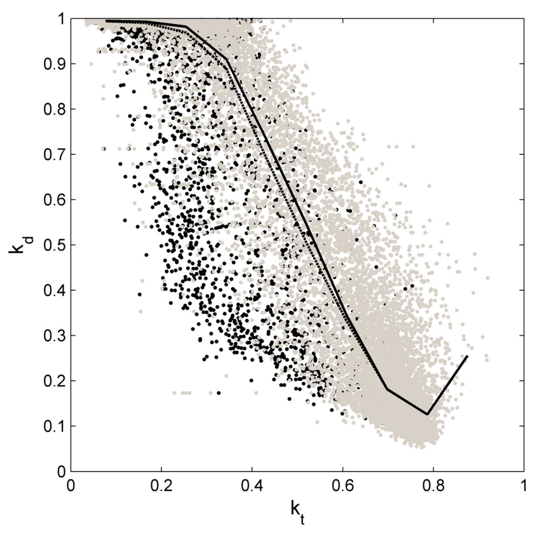
In the experimental kt–kd scatterplot of Figure 2, the observations affected by orographic shadows (black dots) clearly display a distribution rather different from the rest of the data (grey dots). Indeed, a large portion of the black dots lies in the lower-left half of the scatterplot, along the left edge of the grey cloud. This behavior depends on the fact that orographic shadowing implies systematically lower values of GHI, and hence of kt, under all sky conditions (but especially under clear skies). It is evident that approximating the kt–kd relationship with a curve (cf. the median of the distribution) causes the loss of a rather significant part of the variability observed in the data. Notice also that, although including the observations affected by orographic shadows would introduce additional scattering in the plot, it would not modify the median much because of their relative scarcity in the dataset (2098 vs 10,310 points). However, the application of the decomposition models only to the observations affected by orographic shadows returns unacceptably high errors. As a matter of fact, averaged over the 13 literature models being compared, the MBE results for DHI equal 27% (instead of 7%, for the observations free from orographic shadows), the MAE results equal 35% (instead of 27%), and the RMSE is 50% (instead of 37%). On the other hand, the corresponding average errors on DNI are, respectively, MBE = −21% (instead of −3%), MAE = 41% (instead of 14%) and RMSE = 58% (instead of 20%).
Apart from orographic shadowing, complex terrain also reduces incoming diffuse radiation, with respect to flat terrain, as a consequence of smaller SVFs. Under the simplified assumption of isotropic diffuse sky model [68], kd for a non-unitary SVF (kd,SVF≠1) can be estimated as:
k d , S V F 1 = k d , S V F = 1 S V F ( 1 k d , S V F = 1 ( 1 S V F ) )
The (negative) difference between kd,SVF≠1 and kd,SVF=1 (i.e., kd over flat terrain) increases for decreasing SVF, and is larger for intermediate kt and kd values. In the kt–kd scatterplot, this would imply an increase in the slope of the central section of the experimental cloud, accompanied by an overall shift of the points towards the lower-left corner of the diagram. According to these approximate considerations, the kd values observed at Bolzano are up to 18% lower (for kt ≈ 0.8, i.e., under clear-sky conditions) than what would be correspondingly observed over flat terrain. However, the influence of the local SVF on the final estimates of DHI and DNI is difficult to assess in general terms, for it depends both on the number and the magnitude of the GHI observations falling within different kt intervals, i.e., on GHI frequency distribution. Notice that, to the authors’ knowledge, no systematic analysis of the SVF influence on diffuse-beam radiation decomposition is presently available in the literature. Moreover, it is very likely that SVF ≈ 1 for the majority of the (high-quality) radiometric stations used in the literature for the calibration of decomposition models, which, on the other hand, are often applied also in regions characterized by complex orography.

3.3. Comparison of the Decomposition Models

3.3.1. Accuracy of the Models

Table 3 and Table 4 contain the summary statistics resulting from the application of the different decomposition models to the data from Bolzano station. All parameters are calculated on the basis of DHI or DNI estimates and the corresponding observed values (i.e., not in terms of kd or kb errors), for the primary interest is the accuracy of the final radiation estimates. The majority of the models overestimates the diffuse radiation, and many models (namely ORGILL, REINDL-II, SKARTVEIT-I and II and BRL; see Table 3) return rather significant positive average biases, around or above 10%. In particular, the MBE varies from −6% (RUIZ-II) to 19% (SKARTVEIT-I). In contrast, the models tend to underestimate the beam radiation, with MBEs ranging from −9% (SKARTVEIT-I) to 4% (RUIZ-II; see Table 4). As a matter of fact, SKARTVEIT-I, BRL, ORGILL, and REINDL-I and II return negative biases of magnitudes exceeding 5%. On the other hand, the ranges of MAE for DHI and DNI are 22–31% and 12–17%, respectively, and RMSEs for DHI and DNI vary between 32–41% and 17–23%, respectively. In general, the relative accuracy of the decomposition models for the Bolzano dataset appears higher for DNI than for DHI, with values in good accord with what reported by other comparative studies dealing with hourly irradiation data (RMSE for DHI is 35–38% in [29] and 29–38% in [17]; RMSE for DNI is 20–22% in [28], 25–32% in [31], 14–34% in [63], and 20–32% in [32]).
It appears clear that including a variability/persistence index among the predictors typically allows the most accurate estimates. This is the case for the DIRINT and SKARTVEIT-II models, which provide the smallest MAEs and RMSEs among the literature models for both DHI and DNI. Nonetheless, both models show non-negligible MBEs for DHI (6% and 10%, respectively), larger than those of many simpler models. Among the literature models not including a variability index, DISC gives the best results, together with the lowest MBEs (3% for DHI and 1% for DNI), and can be considered the third most accurate model. In contrast, according to the error statistics, the worst-performing models are SKARTVEIT-I for diffuse radiation and ORGILL for beam radiation. In general, it can be concluded that the accuracy of the different models, in terms of MAE and RMSE, does not vary much despite the very different degrees of complexity of the models. In particular, it is not always true that a single-predictor model performs worse than a model with multiple predictors (cf. for example REINDL-I versus REINDL-II, or the bad results of BRL with respect to many single-predictor models).
The three locally-calibrated models (whose coefficients are reported in Table 5) have null DHI biases and almost negligible DNI biases (see Table 3 and Table 4), allowing the accurate assessment of the solar resource, a requirement which is not satisfied by the best-performing literature models (DIRINT and SKARTVEIT-II). However, in terms of MAE and RMSE, both RUIZ-I-loc. and RUIZ-II-loc. only marginally improve the results with respect to their original versions, and do not bring very satisfactory results. On the other hand, the BRL-loc. model produces rather interesting results: apart from zeroing the biases, it returns MAE and RMSE values fully comparable with those of the best-performing models. Consequently, BRL-loc. ranks as the most accurate decomposition model for the Bolzano dataset. Furthermore, consisting of a single equation, the BRL model is not only easy to fit to local data, but also computationally inexpensive, differently from DIRINT and SKARTVEIT-II, which require solving large sets of equations.

3.3.2. Goodness-of-Fit of the Models

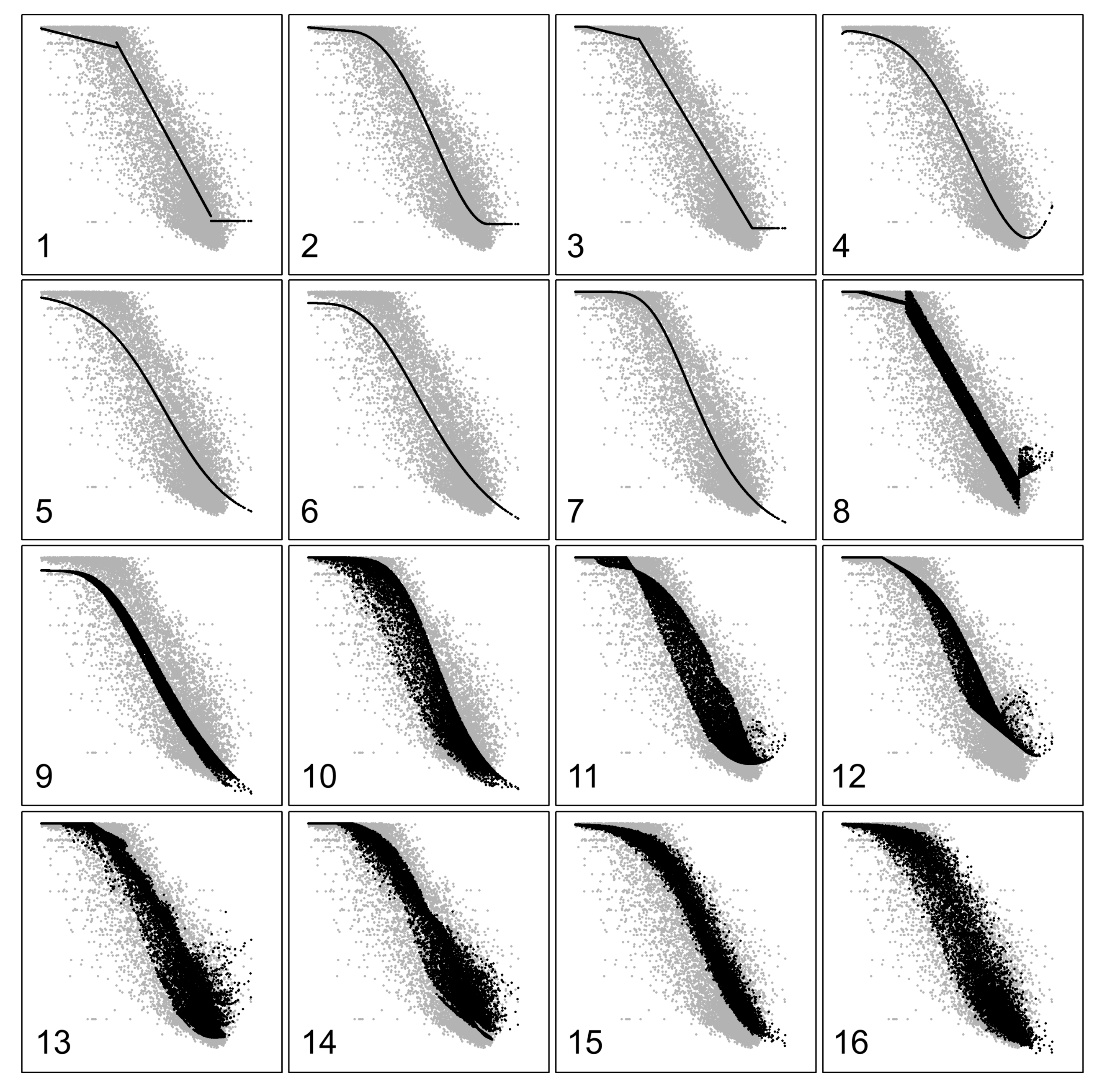
Besides accuracy, the goodness-of-fit of the different algorithms was also tested. In particular, the correlation coefficient for DHI varies between 0.803 (RUIZ-I-loc.) and 0.870–0.871 (SKARTVEIT-II and DIRINT; Table 3), while for DNI it varies between 0.954 (ORGILL and REINDL-I) and 0.971–0.972 (SKARTVEIT-II and DIRINT; Table 4). The locally-calibrated model BRL-loc. returns among the highest R values, immediately followed by DISC. Similarly to R, the modeling efficiency is also rather good for all models, and generally higher for DNI than for DHI. According to E, the worst performances correspond to SKARTVEIT-I (DHI) and ORGILL (DNI) models, while the best results are provided by DIRINT, BRL-loc., and SKARTVEIT-II. The fraction of variance unexplained is in general rather large for DHI (up to 60%) and much smaller for DNI (always below 10%). The models with the smallest FVU are BRL-loc., DISC, and DIRINT for diffuse radiation (8–12%), and DIRINT, BRL-loc., and SKARTVEIT-II for beam radiation (6%). Indeed, the presence of a variability/persistence index among the model predictors is found again to correspond to the best performances. More generally, as expected, increasing the number of predictors brings significant improvements, with single-predictor models performing poorly especially in terms of FVU. From a qualitative point of view, the kt–kd scatterplots in Figure 3 clearly show that multiple predictors allow a better reproduction of the scattering and the shape of the experimental cloud, especially for the BRL-loc. model, whose estimates cover almost the entire spread of the data. On the contrary, simply approximating the kt–kd relationship with a curve (i.e., using a single-predictor algorithm) leaves high levels of unexplained residual variability. However, simply increasing the number of model predictors may not be necessarily the best approach: under the principle of parsimony, in general the use of each additional predictor must be justified by performing appropriate statistical tests, such as, for example, a partial F-test or a selection based on some information criteria (cf. for example the analysis carried out by [68]).
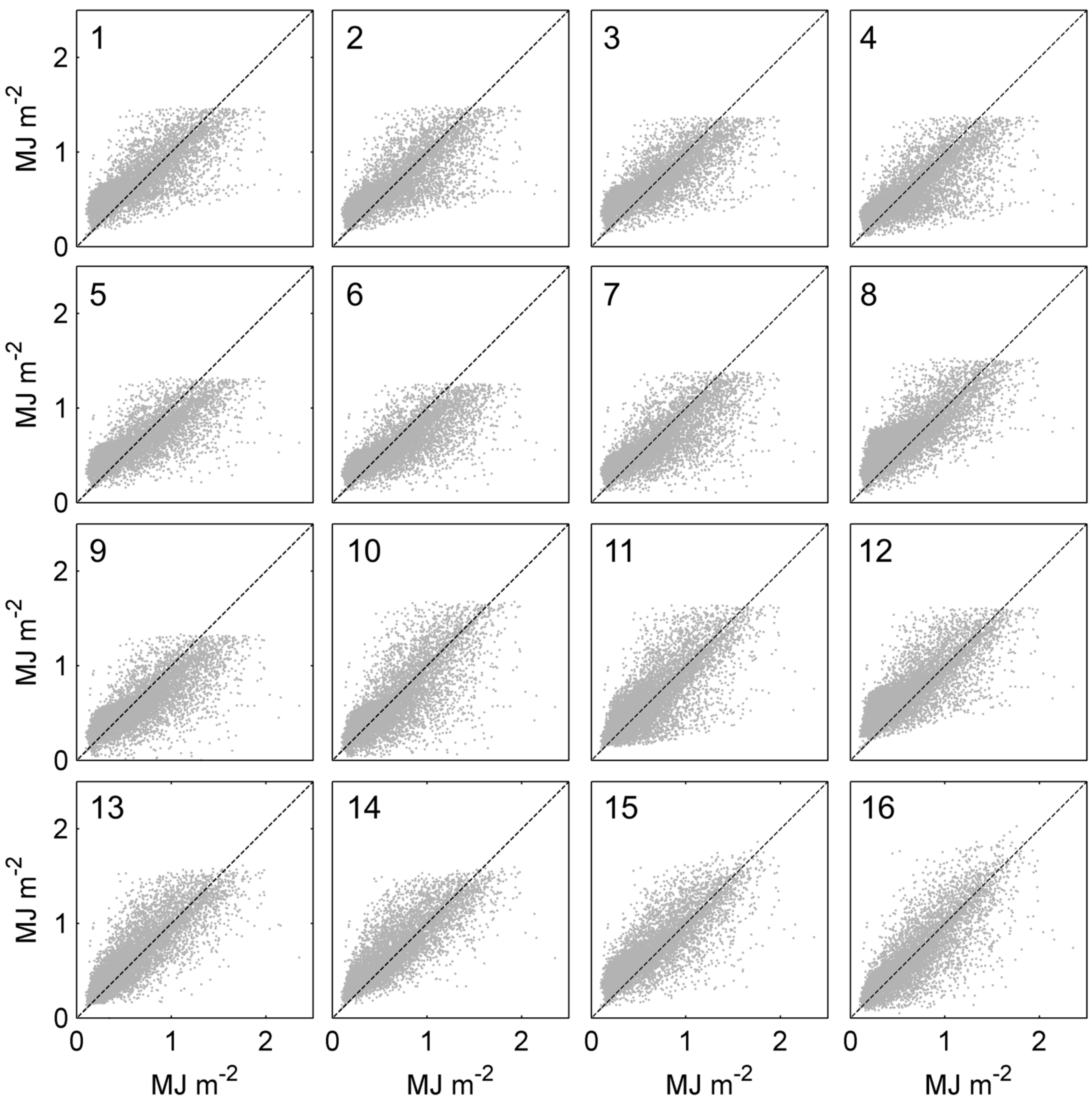
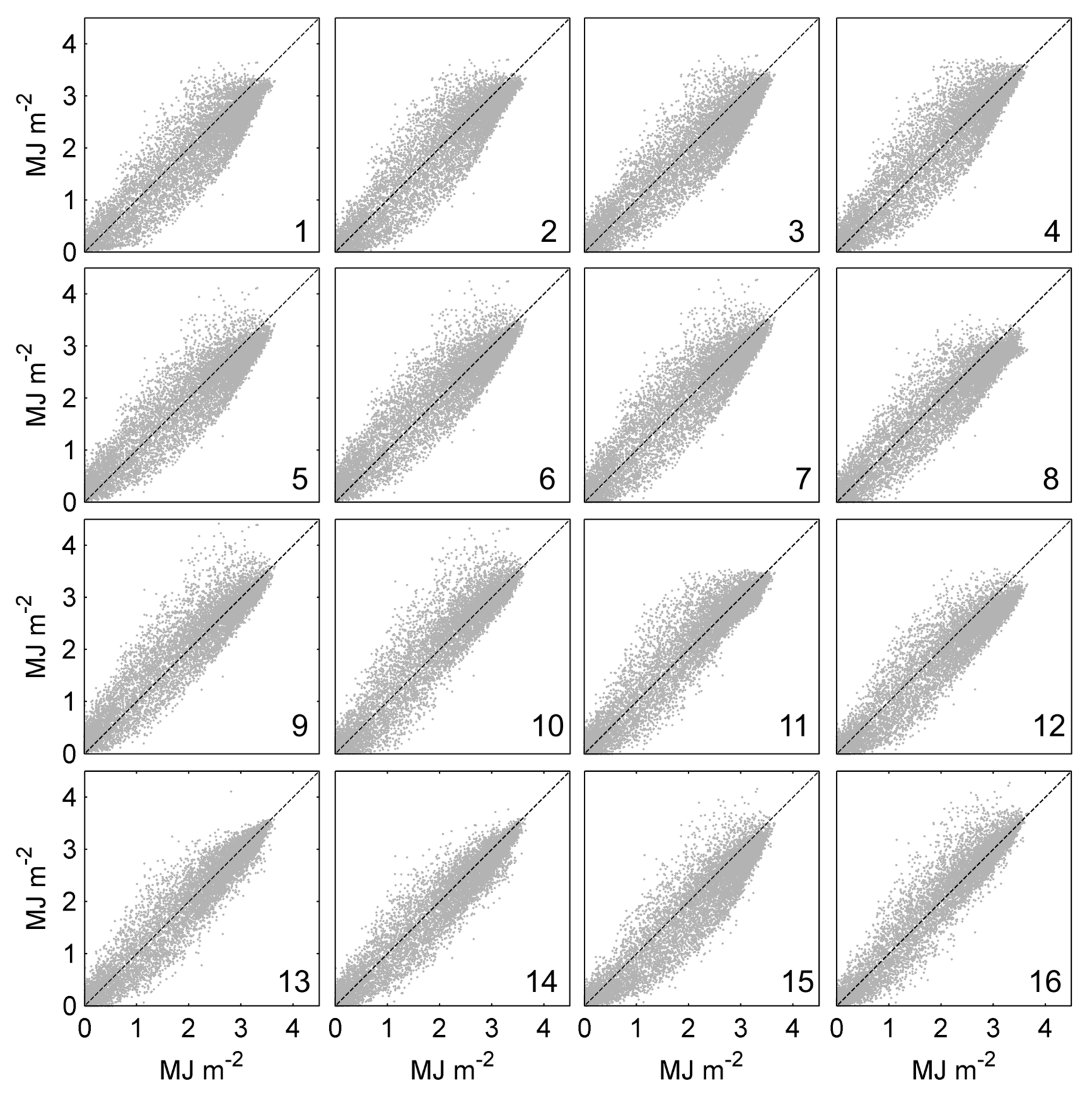
The scatterplots of DHI observations and estimates in Figure 4 reveal that the majority of the models (all except DISC, DIRINT, SKARTVEIT-II, and BRL-loc.) have a common deficiency: they display a pronounced cluster of overestimated values (i.e., points lying above the diagonal) for values of DHI approximately below 0.8 MJ m−2, as observed also by [29] (cf. their Figures 9 and 10). Correspondingly, for high values of measured DNI (above 2 MJ m−2), many models show a dense cluster of underestimated values (i.e., points lying below the diagonal line; see Figure 5).
This is due to the fact that the models do not capture correctly the minimum of the kd distribution found at kt values around 0.8 (cf. Figure 3). Accordingly, under clear-sky conditions these models provide too high DHI and too low DNI with respect to Bolzano observations. This might depend on the specific radiation climatology at the stations considered for the calibration of the literature models (e.g., higher turbidity than at Bolzano). At the same time, a relevant number of outliers corresponding to DNI overestimates (and associated DHI underestimates) in the high kt region is also observed in the scatterplots of Figure 5. The latter behavior is amenable to an incorrect (or lacking) modeling of the diffuse radiation enhancement by scattered clouds under clear-sky conditions [33]. Indeed, the functional form of many models goes to 0 (TORRES, RUIZ-I and II, BRL) or remains constant (ORGILL, ERBS, REINDL-I) for kt tending to 1 (see Figure 3). This issue is almost absent only in the DNI scatterplots of DIRINT and SKARTVEIT-II models, which reproduce the cloud enhancement at best. In addition, for many models the DHI estimates appear superiorly limited to maximum values of 1.3 to 1.8 MJ m−2 (Figure 4). This also may be explained by the fact that the experimental points corresponding to the maximum observed DHI (i.e., the points lying along the upper edge of the experimental cloud) are not caught well, predicting kd values lower than expected. This is particularly pronounced for LOUCHE, TORRES, RUIZ-I, and RUIZ-II models (cf. Figure 3).
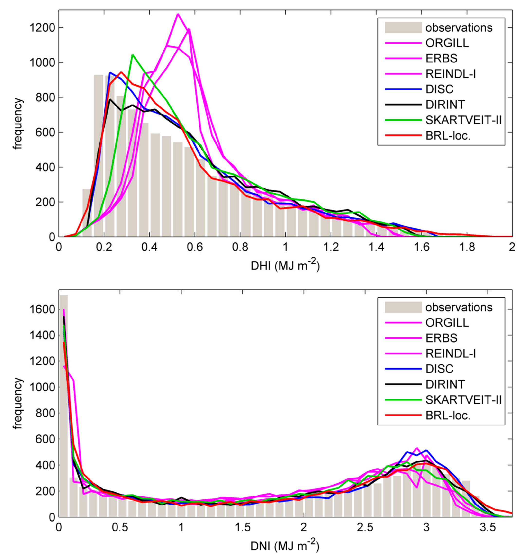
The frequency distributions of DHI and DNI observations and estimates (shown in Figure 6 for a set of selected models) further highlight that the BRL-loc. model matches the observed distributions very well, comparably to DISC and DIRINT models. In contrast, the rest of the models (especially those with a single predictor, in magenta in the figure) display DHI distribution peaks that are too elevated and shifted towards high values (leading to significant frequency discrepancies for DHI < 0.8 MJ m−2), corresponding to badly-modelled frequencies, especially for the lowest and the highest DNI values (i.e., below 0.3 and above 2.3 MJ m−2). These considerations are confirmed by the quantitative results of the KSI test, which indicates that the models returning the cumulative frequency distributions more similar to the observed distributions are DISC and BRL-loc. for diffuse radiation, and BRL-loc. and DIRINT for beam radiation. In contrast, the majority of the other models returned KSI values well above the 100% threshold, corresponding to frequency distributions very different from those of the observations (cf. Table 3 and Table 4).

3.4. Model Results under Different Sky Conditions

In order to explore the performance of the models under different weather conditions, the decomposition results have also been assessed separately for three kt intervals, respectively corresponding to overcast (0 < kt ≤ 0.3), partially cloudy (0.3 < kt ≤ 0.7), and clear sky (kt > 0.7) conditions. The (generally overestimated) kd coefficient shows smaller errors for overcast and clear-sky conditions (average RMSE = 21%) and larger errors under a partly cloudy sky (32%). On the other hand, the (typically underestimated) kb is predicted with better accuracy than kd, with an average RMSE of 7% for an overcast sky, 22% for a partly cloudy sky, and 20% for a clear sky (not shown). Partly cloudy conditions appear the most problematic category for the decomposition of global radiation, as they are characterized by the highest level of scattering (cf. Figure 2).
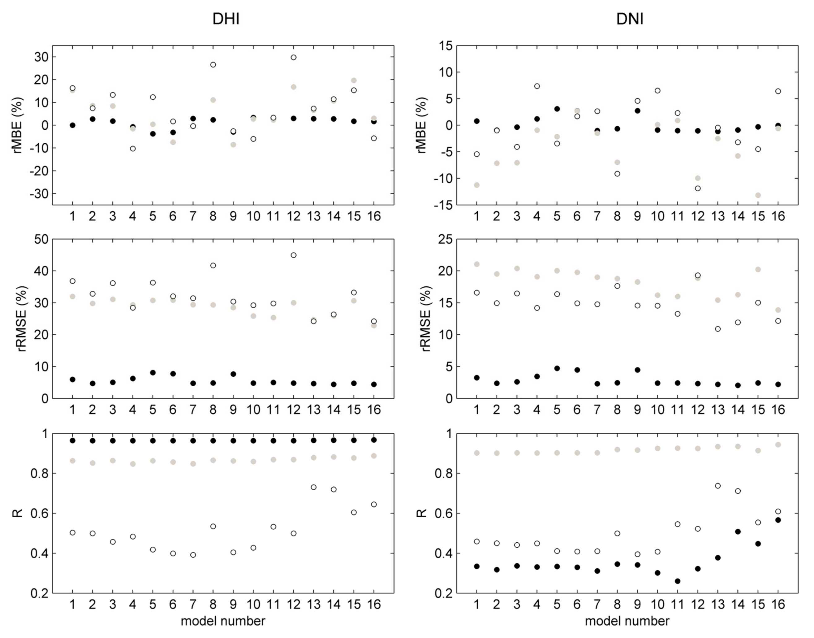
However, when the error statistics are evaluated in terms of hourly irradiances rather than of a-dimensional coefficients (see Figure 7), DHI displays higher errors under clear-sky conditions (average RMSE = 43%) than under partly cloudy conditions (RMSE = 37%), while relative errors for DNI are comparable with those calculated for kb. The discrepancy between relative errors for DHI and kd may be explained by the fact that, while kb values are very well correlated with the distribution of DNI and extraterrestrial radiation (correlation coefficients equal to 0.999 and 0.831), this is not true for kd, DHI, and GHI (correlation coefficients of 0.462 and −0.668).
In general, both diffuse and beam radiation MBEs (in absolute value) are the smallest in the lowest kt interval, i.e., under overcast skies. In particular, the BRL-loc. model shows almost negligible biases under overcast and partly cloudy conditions, but a negative and a positive MBE, respectively, for DHI and DNI under clear skies (see Figure 7). Indeed, despite being calibrated on local data, due to its formulation the model is not able to reproduce observations for clear skies when diffuse radiation is enhanced by scattered clouds (cf. Section 3.3.2). The increasing complexity of the models, from one to multiple predictors, allows the reduction of the errors in the intermediate and high kt range, more evidently when kt variability/persistence is included among the predictors (BRL model excluded; cf. Figure 3). On the other hand, using a variability index accounting for inhomogeneous clouds improves the model performances substantially, not only in terms of correlation coefficient R under clear-sky conditions (i.e., precisely when diffuse radiation enhancement occurs), but also under overcast skies in the case of DNI (see Figure 7). Indeed, while diffuse radiation observations and estimates under overcast and partially-cloudy conditions are already well-correlated and well-explained by the single-predictor models (cf. R, E and FVU values), for beam radiation this is true only for partially-cloudy skies.

4. Conclusions

A set of 13 decomposition models was assessed against a database of 10,310 hourly observations of GHI, DHI, and DNI collected at the Bolzano airport weather station, situated at the floor of one of the major valleys in the eastern Italian Alps. The primary aim of the work was to assess the suitability of commonly-used decomposition models for radiation data collected at an Alpine valley site, characterized by a complex orography and a radiation climatology typical of mountain valleys.
The main findings of the study may be summarized as follows.
  • Observations affected by orographic shadows present a kt–kd distribution very different from the rest of the data and high decomposition errors. Although they do not alter too much the overall decomposition results (because of their relative scarcity), these data are excluded from further analyses. Also, the modification of kd according to the local SVF value is found to be potentially significant for the results of the decomposition models at Alpine sites.
  • Concerning the overall decomposition accuracy, in general, the literature models overestimate the measured DHI (with positive biases often exceeding 10%) and underestimate DNI (with negative biases often above 5%). With respect to MAE and RMSE, the average accuracy of the literature models is around 27% and 37% for DHI, and 14% and 20% for DNI, i.e., comparable to the values obtained by similar studies carried out for flat, homogeneous regions. The use of additional predictors generally (but not always) implies better model performances, especially when a variability/persistence index is included (cf. [33]).
  • Confirming results previously reported in the literature, DIRINT and SKARTVEIT-II are the best-performing models, although they provide non-negligible biases (cf. [33]). The third best model, DISC, shows the lowest bias among the literature models (3%) and a frequency distribution very similar to the observed one (like DIRINT). On the other hand, SKARTVEIT-I (included in the HelioMont algorithm, which provides satellite-based radiation estimates for the Alps [26]) and ORGILL are the worst-performing models, respectively, for diffuse and beam radiation.
  • Apart from a null bias, the local calibration of BRL is found to allow performances comparable or even better than those of DIRINT and SKARTVEIT-II (for DHI: MAE = 20%, RMSE = 32%; for DNI: MAE = 12%, RMSE = 17%). Moreover, BRL is much simpler and is computationally inexpensive (cf. also the recent results from the application and adjustment of the BRL model to hourly and minute data in Brazil [69]).
  • All models reproduce more accurately the observations relative to overcast conditions than those corresponding to partially cloudy and clear skies. Including a variability (or intermittency)/persistence index among the predictors improves the modeling of the cloud-related enhancement of diffuse radiation under clear skies (scattered clouds) [33,70,71].
In view of further improving the estimates of beam and diffuse radiation, the use of additional predictors accounting for atmospheric turbidity (like aerosol or water vapor content; cf. [21,72,73]) in decomposition models would potentially be an option (see also [22]). However, measurements of these atmospheric parameters are not easily available for many weather stations—especially aerosol content, which is very rarely measured routinely or with high temporal resolution. Moreover, a decomposition model is expected to require as few parameters as possible, in order to ensure wide applicability. Considering that the scarcity of meteorological observations is particularly severe in mountainous areas, the number of predictors should be ideally maintained as low as possible, including only the most commonly available meteorological quantities. In addition to the identification of new predictors, or to the development of better model formulations, the influence of complex orography on decomposition results should also be further investigated for applications in mountainous regions. At the same time, more measurements of the diffuse and beam radiation components are needed for a more comprehensive and conclusive evaluation of decomposition models (as well as of radiative transfer and numerical weather prediction models) in the Alpine area, where, currently, available solar datasets still suffer from high levels of uncertainty ([25,36]). Indeed, accurate solar radiation inputs are crucial for a series of meteorological applications, such as surface energy budgets, and their effects on atmospheric boundary layer processes and turbulence [36,74,75,76], including air pollution dispersion and transport [47,48,49], as well as the development of atmospheric convection and thermally-driven winds over complex terrain [39,40,41,42,43,46,77,78,79,80,81,82,83]. To this respect, the usefulness of the locally-calibrated decomposition model could be tested, e.g., for the assessment of the solar resource in the surrounding Alpine valleys (cf. [57]), as well as for the improvement of local solar radiation forecasts, in connection with weather forecasting schemes based on climatological analogs for the region of interest (e.g., [84,85]).

Acknowledgments

This work follows from the project “Climate Atlas of Trentino”, promoted by the Trentino Climate Observatory (www.climatrentino.it) and funded by the Autonomous Province of Trento. Giorgio Belluardo and David Moser acknowledge the European Regional Development Fund for financing the 2-1a-97 PV Initiative.

Author Contributions

L.L., L.G., D.Z., G.B. and D.M. conceived and designed the study; G.B. and D.M. collected and provided the set of data for the study; L.L performed the calculations and analyzed the dataset; L.G., D.Z., G.B., and D.M. contributed to the interpretation of the results; L.L wrote the paper; L.G., D.Z., G.B., and D.M. revised the paper.

Conflicts of Interest

The authors declare no conflict of interest.

References

  1. Huld, T.; Paietta, E.; Zangheri, P.; Pinedo Pascua, I. Assembling Typical Meteorological Year Data Sets for Building Energy Performance Using Reanalysis and Satellite-Based Data. Atmosphere 2018, 9, 53. [Google Scholar] [CrossRef]
  2. Gueymard, C.A. Direct and indirect uncertainties in the prediction of tilted irradiance for solar engineering applications. Sol. Energy 2009, 83, 432–444. [Google Scholar] [CrossRef]
  3. Grigiante, M.; Mottes, F.; Zardi, D.; de Franceschi, M. Experimental solar radiation measurements and their effectiveness in setting up a real-sky irradiance model. Renew. Energy 2011, 36, 1–8. [Google Scholar] [CrossRef]
  4. Myers, D.R. Solar radiation modeling and measurements for renewable energy applications: Data and model quality. Energy 2005, 30, 1517–1531. [Google Scholar] [CrossRef]
  5. Paulescu, M.; Paulescu, E.; Gravila, P.; Badescu, V. Weather Modeling and Forecasting of PV Systems Operation, 1st ed.; Springer: London, UK, 2013; p. 358. ISBN 978-1-4471-4649-0. [Google Scholar] [CrossRef]
  6. Castro-Diez, Y.; Alados-Arboledas, L.; Jiménez, J.I. A model for climatological estimations of global, diffuse, and direct solar radiation on a horizontal surface. Sol. Energy 1989, 42, 417–424. [Google Scholar] [CrossRef]
  7. El-Metwally, M. Simple new methods to estimate global solar radiation based on meteorological data in Egypt. Atmos. Res. 2004, 69, 217–239. [Google Scholar] [CrossRef]
  8. Boata, R.S.; Gravila, P. Functional fuzzy approach for forecasting daily global solar irradiation. Atmos. Res. 2012, 112, 79–88. [Google Scholar] [CrossRef]
  9. Pandey, P.K.; Soupir, M.L. A new method to estimate average hourly global solar radiation on the horizontal surface. Atmos. Res. 2012, 114–115, 83–90. [Google Scholar] [CrossRef]
  10. Manzano, A.; Martín, M.L.; Valero, F.; Armenta, C. A single method to estimate the daily global solar radiation from monthly data. Atmos. Res. 2015, 166, 70–82. [Google Scholar] [CrossRef]
  11. Liu, B.Y.H.; Jordan, R.C. The interrelationship and characteristic distribution of direct, diffuse and total solar radiation. Sol. Energy 1960, 4, 1–19. [Google Scholar] [CrossRef]
  12. Orgill, J.F.; Hollands, K.G.T. Correlation equation for hourly diffuse radiation on a horizontal surface. Sol. Energy 1977, 19, 357–359. [Google Scholar] [CrossRef]
  13. Erbs, D.G.; Klein, S.A.; Duffie, J.A. Estimation of the diffuse radiation fraction for hourly, daily and monthly-average global radiation. Sol. Energy 1982, 28, 293–302. [Google Scholar] [CrossRef]
  14. Skartveit, A.; Olseth, J.A. A model for the diffuse fraction of hourly global radiation. Sol. Energy 1987, 38, 271–274. [Google Scholar] [CrossRef]
  15. Reindl, D.T.; Beckman, W.A.; Duffie, J.A. Diffuse fraction correlations. Sol. Energy 1990, 45, 1–7. [Google Scholar] [CrossRef]
  16. Louche, A.; Notton, G.; Poggi, P.; Simonnot, G. Correlations for direct normal and global horizontal irradiation on a French Mediterranean site. Sol. Energy 1991, 46, 261–266. [Google Scholar] [CrossRef]
  17. Torres, J.L.; De Blas, M.; García, A.; de Francisco, A. Comparative study of various models in estimating hourly diffuse solar irradiance. Renew. Energy 2010, 35, 1325–1332. [Google Scholar] [CrossRef]
  18. Ruiz-Arias, J.A.; Alsamamra, H.; Tovar-Pescador, J.; Pozo-Vázquez, D. Proposal of a regressive model for the hourly diffuse solar radiation under all sky conditions. Energ. Convers. Manag. 2010, 51, 881–893. [Google Scholar] [CrossRef]
  19. Lauret, P.; Boland, J.; Ridley, B. Bayesian statistical analysis applied to solar radiation modelling. Renew. Energy 2013, 49, 124–127. [Google Scholar] [CrossRef]
  20. Maxwell, E.L. A Quasi-Physical Model for Converting Hourly Global Horizontal to Direct Normal Insolation; Report SERI/TR-215-3087; Solar Energy Research Institute: Golden, CO, USA, 1987. [Google Scholar]
  21. Perez, R.; Ineichen, P.; Maxwell, E.; Seals, R.; Zelenka, A. Dynamic global-to-direct irradiance conversion models. ASHRAE Trans. 1992, 3578, 354–369. [Google Scholar]
  22. Skartveit, A.; Olseth, J.A.; Tuft, M.E. An hourly diffuse fraction model with correction for variability and surface albedo. Sol. Energy 1998, 63, 173–183. [Google Scholar] [CrossRef]
  23. Remund, J.; Müller, S.C. Solar Radiation and Uncertainty Information of Meteonorm 7. In Proceedings of the 26th European Photovoltaic Solar Energy Conference and Exhibition, Hamburg, Germany, 5–9 September 2011; pp. 4388–4390. [Google Scholar] [CrossRef]
  24. Blanc, P.; Gschwind, B.; Lefèvre, M.; Wald, L. The HelioClim Project: Surface Solar Irradiance Data for Climate Applications. Remote Sens. 2011, 3, 343–361. [Google Scholar] [CrossRef] [Green Version]
  25. Šúri, M.; Remund, J.; Cebecauer, T.; Dumortier, D.; Wald, L.; Huld, T.; Blanc, P. First Steps in the Cross-Comparison of Solar Resource Spatial Products in Europe. In Proceedings of the EUROSUN 2008—1st International Conference on Solar Heating, Cooling and Buildings, Lisbon, Portugal, 7–10 October 2008. [Google Scholar]
  26. Stöckli, R. The HelioMont Surface Radiation Processing; Scientific Report, 93; Federal Office of Meteorology and Climatology, MeteoSwiss: Zurich, Switzerland, 2013; p. 122. [Google Scholar]
  27. Olmo, F.J.; Batlles, F.J.; Alados-Arboledas, L. Performance of global to direct/diffuse decomposition models before and after the eruption of Mt. Pinatubo, June 1991. Sol. Energy 1996, 57, 433–443. [Google Scholar] [CrossRef]
  28. Batlles, F.J.; Rubio, M.A.; Tovar, J.; Olmo, F.J.; Alados-Arboledas, L. Empirical modeling of hourly direct irradiance by means of hourly global irradiance. Energy 2000, 25, 675–688. [Google Scholar] [CrossRef]
  29. Notton, G.; Cristofari, C.; Muselli, M.; Poggi, P. Calculation on an hourly basis of solar diffuse irradiations from global data for horizontal surfaces in Ajaccio. Energy Convers. Manag. 2004, 45, 2849–2866. [Google Scholar] [CrossRef]
  30. Jacovides, C.P.; Tymvios, F.S.; Assimakopoulos, V.D.; Kaltsounides, N.A. Comparative study of various correlations in estimating hourly diffuse fraction of global solar radiation. Renew. Energy 2006, 31, 2492–2504. [Google Scholar] [CrossRef]
  31. Ineichen, P. Comparison and validation of three global-to-beam irradiance models against ground measurements. Sol. Energy 2008, 82, 501–512. [Google Scholar] [CrossRef]
  32. Bertrand, C.; Vanderveken, G.; Journée, M. Evaluation of decomposition models of various complexity to estimate the direct solar irradiance over Belgium. Renew. Energy 2015, 74, 618–626. [Google Scholar] [CrossRef]
  33. Gueymard, C.A.; Ruiz-Arias, J.A. Performance of Separation Models to Predict Direct Irradiance at High Frequency: Validation over Arid Areas. In Proceedings of the EUROSUN 2014—International Conference on Solar Energy and Buildings, Aix-Les-Bains, France, 16–19 September 2014. [Google Scholar]
  34. Gueymard, C.A.; Ruiz-Arias, J.A. Extensive worldwide validation and climate sensitivity analysis of direct irradiance predictions from 1-min global irradiance. Sol. Energy 2016, 128, 1–30. [Google Scholar] [CrossRef]
  35. Tovar, J.; Olmo, F.J.; Alados-Arboledas, L. Local-Scale Variability of Solar Radiation in a Mountainous Region. J. Appl. Meteorol. 1995, 34, 2316–2322. [Google Scholar] [CrossRef]
  36. Huld, T.; Müller, R.; Gambardella, A. A new solar radiation database for estimating PV performance in Europe and Africa. Sol. Energy 2012, 86, 1803–1815. [Google Scholar] [CrossRef]
  37. Šúri, M.; Huld, T.A.; Dunlop, E.D.; Ossenbrink, H.A. Potential of solar electricity generation in the European Union member states and candidate countries. Sol. Energy 2007, 81, 1295–1305. [Google Scholar] [CrossRef]
  38. Castelli, M.; Stöckli, R.; Zardi, D.; Tetzlaff, A.; Wagner, J.E.; Belluardo, G.; Zebisch, M.; Petitta, M. The HelioMont method for assessing solar irradiance over complex terrain: Validation and improvements. Remote Sens. Environ. 2014, 152, 603–613. [Google Scholar] [CrossRef]
  39. Rampanelli, G.; Zardi, D.; Rotunno, R. Mechanisms of Up-Valley Winds. J. Atmos. Sci. 2004, 61, 3097–3111. [Google Scholar] [CrossRef]
  40. Rotach, M.; Zardi, D. On the boundary layer structure over highly complex terrain: Key findings from MAP. Q. J. R. Meteorol. Soc. 2007, 133, 937–948. [Google Scholar] [CrossRef]
  41. Serafin, S.; Zardi, D. Daytime Heat Transfer Processes Related to Slope Flows and Turbulent Convection in an Idealized Mountain Valley. J. Atmos. Sci. 2010, 67, 3739–3756. [Google Scholar] [CrossRef]
  42. Serafin, S.; Zardi, D. Structure of the atmospheric boundary layer in the vicinity of a developing upslope flow system: A numerical model study. J. Atmos. Sci. 2010, 67, 1171–1185. [Google Scholar] [CrossRef]
  43. Serafin, S.; Zardi, D. Daytime development of the boundary layer over a plain and in a valley under fair weather conditions: A comparison by means of idealized numerical simulations. J. Atmos. Sci. 2011, 68, 2128–2141. [Google Scholar] [CrossRef]
  44. Zardi, D.; Whiteman, C.D. Diurnal mountain wind systems. In Mountain Weather Research and Forecasting—Recent Progress and Current Challenges; Chow, K.F., De Wekker, S.F.J., Snyder, J.B., Eds.; Springer: Dordrecht, The Netherlands, 2013; pp. 35–119. [Google Scholar] [CrossRef]
  45. Zardi, D.; Serafin, S. An analytic solution for daily-periodic thermally-driven slope flow. Q. J. R. Meteorol. Soc. 2015, 141, 1968–1974. [Google Scholar] [CrossRef]
  46. Giovannini, L.; Laiti, L.; Serafin, S.; Zardi, D. The thermally driven diurnal wind system of the Adige Valley in the Italian Alps. Q. J. R. Meteorol. Soc. 2017, 143, 2389–2402. [Google Scholar] [CrossRef]
  47. De Franceschi, M.; Zardi, D. Study of wintertime high pollution episodes during the Brenner-South ALPNAP measurement campaign. Meteorol. Atmos. Phys. 2009, 103, 237–250. [Google Scholar] [CrossRef]
  48. Rada, E.C.; Ragazzi, M.; Zardi, D.; Laiti, L.; Ferrari, A. PCDD/F environmental impact from municipal solid waste bio-drying plant. Chemosphere 2011, 84, 289–295. [Google Scholar] [CrossRef] [PubMed]
  49. Ragazzi, M.; Tirler, W.; Angelucci, G.; Zardi, D.; Rada, E.C. Management of atmospheric pollutants from waste incineration processes: The case of Bozen. Waste Manag. Res. 2013, 31, 235–240. [Google Scholar] [CrossRef] [PubMed]
  50. Grenier, J.C.; De La Casinière, A.; Cabot, T. Atmospheric Turbidity Analyzed by Means of Standardized Linke’s Turbidity Factor. J. Appl. Meteorol. 1995, 34, 1449–1458. [Google Scholar] [CrossRef]
  51. Belluardo, G.; Pichler, M.; Moser, D.; Nikolaeva-Dimitrova, M. One-year comparison of different thin film technologies at Bolzano airport test installation. In Fuelling the Future: Advances in Science and Technologies for Energy Generation, Transmission and Storage; Mendez-Vilas, A., Ed.; BrownWalker Press: Boca Raton, FL, USA, 2012; p. 614. [Google Scholar]
  52. Moser, D.; Pichler, M.; Nikolaeva-Dimitrova, M. Filtering procedures for reliable outdoor temperature coefficients in different photovoltaic technologies. J. Sol. Energy Eng. 2013, 136, 021006. [Google Scholar] [CrossRef]
  53. IEC (International Electrotechnical Commission). International Standard IEC61724: Photovoltaic System Performance Monitoring: Guidelines for Measurement, Data Exchange, and Analysis; IEC: Geneva, Switzerland, 1998. [Google Scholar]
  54. Younes, S.; Claywell, R.; Muneer, T. Quality control of solar radiation data: Present status and proposed new approaches. Energy 2005, 30, 1533–1549. [Google Scholar] [CrossRef]
  55. Journée, M.; Bertrand, C. Quality control of solar radiation data within the RMIB solar measurements network. Sol. Energy 2011, 85, 72–86. [Google Scholar] [CrossRef]
  56. Estévez, J.; Gavilán, P.; García-Marín, A.P.; Zardi, D. A method for detecting spurious precipitation signals from automatic weather stations in irrigated areas. Int. J. Climatol. 2015, 35, 1556–1568. [Google Scholar] [CrossRef]
  57. Laiti, L.; Andreis, D.; Zottele, F.; Giovannini, L.; Panziera, L.; Toller, G.; Zardi, D. A Solar Atlas for the Trentino Region in the Alps: Quality Control of Surface Radiation Data. Energy Proced. 2014, 59, 336–343. [Google Scholar] [CrossRef]
  58. ESRA (European Society of Regional Anaesthesia). European Solar Radiation Atlas, 4th ed.; Greif, J., Scharmer, K., Eds.; Presses de l’Ecole des Mines de Paris: Paris, France, 2000. [Google Scholar]
  59. Rigollier, C.; Bauer, O.; Wald, L. On the clear sky model of the 4th European Solar Radiation Atlas with respect to the Heliosat method. Sol. Energy 2000, 68, 33–48. [Google Scholar] [CrossRef]
  60. Remund, J.; Wald, L.; Page, J. Chain of algorithms to calculate advanced radiation parameters. In Proceedings of the International Solar Energy Society (ISES) Solar World Congress 2003, Göteborg, Sweden, 14–19 June 2003. [Google Scholar]
  61. Linke, F. Transmission-Koeffizient und Trübungsfaktor. Beitr. Phys. Atmos. 1922, 10, 91–103. [Google Scholar]
  62. Nash, J.E.; Suttcliffe, J.V. River flow forecasting through conceptual models, part I. A discussion of principles. J. Hydrol. 1970, 10, 282–290. [Google Scholar] [CrossRef]
  63. Boland, J.; Huang, J.; Ridley, B. Decomposing global solar radiation into its direct and diffuse components. Renew. Sustain. Energy Rev. 2013, 28, 749–756. [Google Scholar] [CrossRef]
  64. Roesch, A.; Wild, M.; Ohmura, A.; Dutton, E.G.; Long, C.N.; Zhang, T. Assessment of BSRN radiation records for the computation of monthly means. Atmos. Meas. Tech. 2011, 4, 339–354. [Google Scholar] [CrossRef] [Green Version]
  65. Photovoltaic Geographical Information System (PVGIS), Geographical Assessment of Solar Resource and Performance of Photovoltaic Technology. Available online: re.jrc.ec.europa.eu/pvgis (accessed on 31 December 2015).
  66. 3PClim—Past, Present and Perspective Climate of Tirol, Südtirol-Alto Adige and Veneto. Available online: www.3pclim.eu (accessed on 31 December 2015).
  67. Liu, B.Y.H.; Jordan, R.C. Daily insolation on surfaces tilted towards the equator. ASHRAE Trans 1962, 67, 526–541. [Google Scholar]
  68. Ridley, B.; Boland, J.; Lauret, P. Modelling of diffuse solar fraction with multiple predictors. Renew. Energy 2010, 35, 478–483. [Google Scholar] [CrossRef]
  69. Lemos, L.F.L.; Starke, A.R.; Boland, J.; Cardemil, J.M.; Machado, R.D.; Colle, S. Assessment of solar radiation components in Brazil using the BRL model. Renew. Energy 2017, 108, 569–580. [Google Scholar] [CrossRef]
  70. Fortuna, L.; Nunnari, G.; Nunnari, S. A new fine-grained classification strategy for solar daily radiation patterns. Pattern Recogit. Lett. 2016, 81, 110–117. [Google Scholar] [CrossRef]
  71. Starke, A.R.; Lemos, L.F.L.; Boland, J.; Cardemil, J.M.; Colle, S. Resolution of the Cloud Enhancement Problem for One-Minute Diffuse Radiation Prediction. Renew. Energy 2018, in press. [Google Scholar] [CrossRef]
  72. Mueller, R.; Träger-Chatterjee, C. Brief Accuracy Assessment of Aerosol Climatologies for the Retrieval of Solar Surface Radiation. Atmosphere 2014, 5, 959–972. [Google Scholar] [CrossRef]
  73. Mueller, R.; Pfeifroth, U.; Traeger-Chatterjee, C. Towards Optimal Aerosol Information for the Retrieval of Solar Surface Radiation Using Heliosat. Atmosphere 2015, 6, 863–878. [Google Scholar] [CrossRef]
  74. De Franceschi, M.; Zardi, D. Evaluation of cut-off frequency and correction of filter-induced phase lag and attenuation in eddy covariance analysis of turbulence data. Bound.-Lay Meteorol. 2003, 108, 289–303. [Google Scholar] [CrossRef]
  75. De Franceschi, M.; Zardi, D.; Tagliazucca, M.; Tampieri, F. Analysis of second order moments in the surface layer turbulence in an Alpine valley. Q. J. R. Meteorol. Soc. 2009, 135, 1750–1765. [Google Scholar] [CrossRef]
  76. Serafin, S.; Adler, B.; Cuxart, J.; De Wekker, S.F.J.; Gohm, A.; Grisogono, B.; Kalthoff, N.; Kirshbaum, D.J.; Rotach, M.W.; Schmidli, J.; et al. Exchange Processes in the Atmospheric Boundary Layer Over Mountainous Terrain. Atmosphere 2018, 9, 102. [Google Scholar] [CrossRef]
  77. Giovannini, L.; Zardi, D.; de Franceschi, M. Analysis of the urban thermal fingerprint of the city of Trento in the Alps. J. Appl. Meteorol. Clim. 2011, 50, 1145–1162. [Google Scholar] [CrossRef]
  78. Giovannini, L.; Zardi, D.; de Franceschi, M. Characterization of the Thermal Structure inside an Urban Canyon: Field Measurements and Validation of a Simple Model. J. Appl. Meteorol. Clim. 2013, 52, 64–81. [Google Scholar] [CrossRef]
  79. Giovannini, L.; Zardi, D.; de Franceschi, M.; Chen, F. Numerical simulations of boundary-layer processes and urban-induced alterations in an Alpine valley. Int. J. Climatol. 2014, 34, 1111–1131. [Google Scholar] [CrossRef]
  80. Laiti, L.; Zardi, D.; de Franceschi, M.; Rampanelli, G. Residual Kriging analysis of airborne measurements: Application to the mapping of Atmospheric Boundary-Layer thermal structures in a mountain valley. Atmos. Sci. Lett. 2013, 14, 79–85. [Google Scholar] [CrossRef]
  81. Laiti, L.; Zardi, D.; de Franceschi, M.; Rampanelli, G. Atmospheric boundary layer structures associated with the Ora del Garda wind in the Alps as revealed from airborne and surface measurements. Atmos. Res. 2013, 132–133, 473–489. [Google Scholar] [CrossRef]
  82. Laiti, L.; Zardi, D.; de Franceschi, M.; Rampanelli, G.; Giovannini, L. Analysis of the diurnal development of a lake-valley circulation in the Alps based on airborne and surface measurements. Atmos. Chem. Phys. 2014, 14, 9771–9786. [Google Scholar] [CrossRef] [Green Version]
  83. Giovannini, L.; Laiti, L.; Zardi, D.; de Franceschi, M. Climatological characteristics of the Ora del Garda wind in the Alps. Int. J. Climatol. 2015, 35, 4103–4115. [Google Scholar] [CrossRef]
  84. Panziera, L.; Giovannini, L.; Laiti, L.; Zardi, D. The relation between circulation types and regional Alpine climate. Part I: Synoptic climatology of Trentino. Int. J. Climatol. 2015, 35, 4655–4672. [Google Scholar] [CrossRef]
  85. Panziera, L.; Giovannini, L.; Laiti, L.; Zardi, D. The relation between circulation types and regional Alpine climate. Part II: The dependence of the predictive skill on the vertical level of the classification for Trentino. Int. J. Climatol. 2016, 36, 2189–2199. [Google Scholar] [CrossRef]
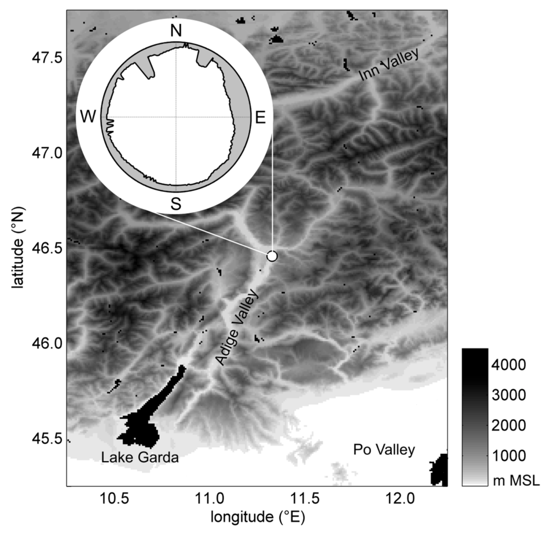
Figure 1. Location of Bolzano station (white dot) in the Eastern Alps and local orography. The horizon elevation profile for the weather station is also shown in the polar plot in the upper left corner.
Atmosphere 09 00117 g001
Figure 2. Scatterplot of kt vs kd for Bolzano station (2011–2014 data). Grey dots represent observations not affected by orographic shadows, while black dots correspond to the hours partially or totally affected by orographic shadows. The median values of kd, calculated for 10 equal-size kt intervals, are shown by the two black lines. The dotted line includes all observations, while the solid line corresponds only to the observations not affected by orographic shadows.
Atmosphere 09 00117 g002
Figure 3. Scatterplots of kt vs. kd for the experimental data (grey dots) and according to the different decomposition models (black dots). See Table 1 for the numbers associated with the models. The axes are the same as in Figure 2 (axes labels not reported for the sake of clarity).
Atmosphere 09 00117 g003
Figure 4. Scatterplots of DHI observations (abscise axis) vs estimates (ordinate axis), according to the compared decomposition models. See Table 1 for the numbers associated with the different models. The black diagonal lines identify the perfect coincidence of observations and estimates.
Atmosphere 09 00117 g004
Figure 5. As in Figure 4, but for direct normal irradiation (DNI) observations and estimates.
Atmosphere 09 00117 g005
Figure 6. Empirical frequency distributions of DHI (upper panel) and DNI (lower panel) according to the best-performing decomposition models (bars show observations; lines show estimates). Three widely-used single-predictor models are also shown for comparison (magenta lines). See Table 1 for the model acronyms.
Atmosphere 09 00117 g006
Figure 7. Performance statistics according to the different models (left: DHI; right: DNI) for three different intervals of kt. Black dots correspond to 0 < kt ≤ 0.3 (4705 data; overcast sky), grey dots to 0.3 < kt ≤ 0.7 (2623 data; partially cloudy sky), and empty dots to kt > 0.7 (2982 data; clear sky). See Table 1 for the numbers associated with the different models.
Atmosphere 09 00117 g007
Table 1. List of the decomposition models, associated model numbers, literature references, acronyms and predictors used (hourly clearness index: kt, local apparent time: t, solar elevation: h, daily clearness index: Kt, variability/persistence index: Ψ).
Model TypeModel NumberAuthor(s) (Year)Model AcronymPredictors
single predictor1Orgill and Hollands (1977) [12]ORGILLkt
2Erbs et al. (1982) [13]ERBSkt
3Reindl et al. (1990) [15]REINDL-Ikt
4Louche et al. (1991) [16]LOUCHEkt
5Torres et al. (2010) [17]TORRESkt
6Ruiz-Arias et al. (2010) [18]RUIZ-Ikt
7local calibration of Ruiz-Arias et al. (2010) [18]RUIZ-I-loc.kt
multiple predictors8Reindl et al. (1990) [15]REINDL-IIkt h
9Ruiz-Arias et al. (2010) [15]RUIZ-IIkt m
10local calibration of Ruiz-Arias et al. (2010) [18]RUIZ-II-loc.kt m
11Maxwell (1987) [20]DISCkt m
12Skartveit and Olseth (1987) [14]SKARTVEIT-Ikt h
with variability predictor13Perez et al. (1992) [21]DIRINTkt h Ψ
14Skartveit et al. (1998) [22]SKARTVEIT-IIkt Ψ
15Lauret et al. (2013) [19]BRLkt t h Kt Ψ
16local calibration of Lauret et al. (2013) [19]BRL-loc.kt t h Kt Ψ
Table 2. Comparison of monthly mean global, diffuse, and beam (normal) daily irradiations (Ig, Id, and Ibn), as well as daily diffuse fractions (kd), calculated from Bolzano experimental data and extracted from PVGIS-CMSAF database.
MonthBolzano ObservationsPVGIS-CMSAF
IgIdIbnkdIgIdIbnkd
Jan.4.812.187.490.455.332.728.030.51
Feb.8.213.5211.360.439.223.8713.030.42
Mar.13.114.6716.350.3614.516.3815.340.44
Apr.16.407.0914.120.4317.757.6316.090.43
May20.757.8217.660.3821.359.1817.350.43
Jun.21.388.3616.330.3922.909.8518.250.43
Jul.21.747.6918.850.3523.658.5121.200.36
Aug.19.396.2319.660.3219.877.3519.120.37
Sep.14.675.0216.510.3415.346.2915.800.41
Oct.9.323.7011.870.409.864.7311.230.48
Nov.4.902.237.260.455.692.967.880.52
Dec.3.731.776.450.484.252.296.880.54
Table 3. Performance statistics for the different decomposition models applied to the Bolzano station data, evaluated over hourly diffuse horizontal irradiation (DHI) values: mean bias error (MBE), mean absolute error (MAE), and root mean square error (RMSE) are in MJ m−2, while relative errors (rMBE, rMAE, and rRMSE, in %) are calculated with respect to the overall mean value of DHI (0.56 MJ m−2). The fraction of variance unexplained (FVU) and Kolmogorov-Smirnov test integral (KSI) (99% confidence interval) are expressed as percentages. The three best-performing models for each indicator are in bold font, and the three worst-performing models are underlined (notice that locally-calibrated models are excluded from the ranking). See Table 1 for the model numbers and acronyms.
ModelMBEMAERMSErMBErMAErRMSEREFVUKSI
1ORGILL0.070.170.2213.2829.5838.690.8200.62239.85284
2ERBS0.040.150.217.3526.9537.230.8170.65041.83246
3REINDL-I0.050.160.219.0128.7538.090.8170.63449.02287
4LOUCHE−0.020.140.21−4.2725.5237.780.8060.64045.96232
5TORRES0.020.160.213.6929.0938.340.8110.62957.09303
6RUIZ-I0.020.150.223.8127.7138.760.8100.62159.43296
7RUIZ-I-loc.0.000.150.210.0026.2937.940.8030.63749.70251
8REINDL-II0.080.170.2214.8429.6338.980.8200.61630.56279
9RUIZ-II−0.030.140.21−5.7425.9337.610.8140.64348.77234
10RUIZ-II-loc.0.000.130.210.0023.7436.970.8170.65513.9695
11DISC0.020.130.202.7123.6835.480.8340.68211.4461
12SKARTVEIT-I0.110.170.2318.9431.0240.710.8200.58221.92303
13DIRINT0.040.120.186.2721.4831.820.8710.74512.21119
14SKARTVEIT-II0.050.130.189.7422.8032.510.8700.73318.20172
15BRL0.090.150.2115.5427.5337.050.8450.65320.66246
16BRL-loc.0.000.120.180.0020.4732.290.8640.7378.4063
Table 4. As in Table 3, but for hourly DNI values. Relative errors are calculated with respect to the overall mean value of DNI (1.71 MJ m−2).
ModelMBEMAERMSErMBErMAErRMSEREFVUKSI
1ORGILL0.130.290.397.5116.8822.550.9540.89810.22241
2ERBS−0.070.260.36−4.1815.4221.200.9560.9109.04128
3REINDL-I−0.090.280.37−5.0616.3921.800.9540.9049.56178
4LOUCHE0.040.260.362.1015.0921.040.9560.9118.9057
5TORRES0.030.280.371.7816.4921.300.9550.9099.12176
6RUIZ-I0.040.270.362.3515.8521.070.9550.9118.93150
7RUIZ-I-loc.0.000.260.36−0.0715.0720.900.9550.9128.7868
8REINDL-II−0.110.270.35−6.7115.9220.700.9620.9148.61208
9RUIZ-II0.070.260.354.3314.9520.540.9590.9158.48150
10RUIZ-II-loc.0.040.230.342.0613.5519.920.9620.9207.9889
11DISC0.020.220.321.0713.0318.610.9650.9306.9670
12SKARTVEIT-I0.160.280.369.2416.4721.200.9640.9109.03277
13DIRINT0.030.200.29-1.6511.9316.800.9720.9435.6755
14SKARTVEIT-II−0.070.220.30-4.1812.6717.340.9710.9406.04132
15BRL0.140.270.378.3615.8021.850.9580.9049.60257
16BRL-loc.0.010.200.300.8111.5317.140.9720.9405.9047
Table 5. Coefficients obtained by local calibration of RUIZ-I, RUIZ-II and BRL models (cf. formulas in Section 2.2). Original coefficients are also reported for comparison. See Table 1 for the model acronyms.
RUIZ-IRUIZ-I-loc.RUIZ-IIRUIZ-II-loc.BRLBRL-loc.
a00.9521.0000.9440.998−5.32−6.67
a11.0411.0711.5381.0187.286.72
a22.3002.6422.8083.244−0.030.06
a3−4.702−5.343−5.759−3.003−0.0047−0.0072
a4--2.276−3.5721.722.01
a5--−0.125−0.4951.082.47
a6--0.0130.035--