Effects of Meteorology Nudging in Regional Hydroclimatic Simulations of the Eastern Mediterranean

Abstract

In this study, we investigated the effects of grid and spectral nudging in regional hydroclimatic simulations over the Eastern Mediterranean climate change hot-spot. We performed year-long simulations for the hydrological year October 2001–September 2002 using the Weather Research and Forecasting (WRF) model at 12-km resolution, driven by the ERA-Interim reanalyses. Six grid and three spectral nudging options were tested using a number of model configurations. Due to the large uncertainty of regional observations, we compared the model with various satellite- and station-based meteorological datasets. The effect of nudging was tested for mean weather conditions and precipitation characteristics and extremes. For certain parts of the study domain, WRF was found to reproduce both aspects of rainfall over the Eastern Mediterranean reasonably well. Our findings highlighted that, for the WRF modeling system, nudging is critical for the simulation of rainfall; however, the application of interior constraint methods was found to have different impacts on various locations and climatic regimes. For the hyperarid parts of the domain, nudging did not improve the simulation of precipitation amounts (about 20% additional drying was introduced), while it added much value for the wetter rainfall regimes of the Eastern Mediterranean (corrections of about 30%). Improvements in the simulated precipitation were mostly introduced by spectral nudging; however, this option required significant computational resources. For these ERA-Interim-driven simulations, grid nudging that involves specific humidity within the planetary boundary layer is not recommended for the simulation of precipitation since it introduces dry biases up to 75–80%.

1. Introduction

Regional climate models (RCMs) are widely used for high-resolution simulations to dynamically downscale the atmospheric circulation computed by global climate models (GCMs) or reanalyses [1]. However, during the downscaling process, the simulation of RCMs tends to drift away from the driving fields [2]. Although the application of lateral boundary conditions (LBCs) constrains RCM simulations, the dynamical formulation and physical parameterizations of RCMs are as nonlinear as those of any GCM, and thus, nested model simulations may exhibit a certain level of freedom and chaotic behavior [3]. This freedom is in part desirable in view of the additional information generated by RCMs, but it can also manifest internal variability, particularly for extended simulation domains. Developing a solution that addresses this issue by retaining the large-scale features (from the large-scale fields) and the small-scale features (from the RCMs) has led to the development of interior constraints or nudging techniques [2]. Nudging involves adding a corrective term to the prognostic equations that is based on the difference between the model state and a reference field [4]. Two main nudging approaches are generally used. One is the indiscriminate or analysis or grid nudging [5] and the second is spectral nudging [6]. The first consists of relaxing the RCM’s prognostic variables towards the GCM values within a predetermined relaxation time and for all scales [7]. This simply means that nudging is applied in every grid cell of the limited area model. In the second (spectral) approach, the nudging term is spectrally expanded in both the zonal and meridional directions and only waves below selected wave numbers are kept in the nudging term. This means that nudging is applied only for the large-scale waves. Another, less common and not so straightforward approach is to concatenate daily simulations to create a “pseudo-continuous” simulation [8,9]. This method is also found to reduce biases, keeping the model close to the forcing fields but still free enough to generate mesoscale and local features. This approach, however, when applied to long climate simulations, could result in the excessive use of computational resources since several periods (hours or days) are simulated more than once to ensure a reasonable duration of model spin-up.

Nudging techniques can be applied at all model levels. However, most of the available literature suggests caution when applying it within the planetary boundary layer (PBL) in order to allow the regional model to reproduce the relatively small- and local-scale processes involved. The strength of nudging for each prognostic variable can be controlled through the nudging coefficients. Discussing the outcomes of the 2nd Lund Regional-Scale Climate Model Workshop, Arrit and Rummukainen [10] highlighted that the optimal scale of nudging is not yet well defined and likely depends on the purpose of application. Some general conclusions of this workshop include that if nudging is too weak, the RCM can still become inconsistent with its large-scale driving data, while if nudging is too strong, the RCM solution is overconstrained and development of the desired fine-scale information can be suppressed. Therefore, the strength of nudging should be carefully selected on a case-by-case basis. Similarly, the results presented in [3] indicate that the use of weak-to-mild nudging may constitute a reasonable compromise between the risk of decoupling of the RCM internal solution from the lateral boundary conditions (without nudging) and an excessive control of the large scales (with strong nudging). In the same context, Bowden et al. [11] suggest that the strength of the nudging coefficients should be minimized for grid nudging to increase the variability at wavelengths that should be resolvable in the RCM.

A number of authors [12,13] showed that such interior constraint methods reduce the influence of the domain size, position, and orientation that are, on one hand, subjectively chosen but, on the other hand, can strongly affect the modeling results. Likewise, Alexandru et al. [3] suggest that large domains may need more control than the one usually provided at the boundaries, while Miguez-Macho et al. [12] recommend large-scale nudging for all downscaling studies with RCMs using domain sizes of a few thousand kilometers and larger, which is the case for the simulation domain of this study and for most ongoing downscaling efforts including the Coordinated Regional Downscaling Experiment—CORDEX (http://www.cordex.org/).

Grid and spectral nudging have been applied and tested for weather/climate simulations in a wide range of limited area models, including MM5 [14,15], WRF [2,4,7,11,16,17], RAMS [12,13], Canadian RCM [3], ALADIN [1], and REMO [6].

A challenging application of such weather/climate modeling techniques is that of the Eastern Mediterranean and Middle East (EMME), as the region is characterized by steep precipitation gradients. The current resolution of global earth system models is not fine enough to accurately represent local weather features related to the complex coastlines, orography, and presence of urban centers and small islands. Therefore, improved and higher-resolution simulations are essential in order to tackle the impacts of climate change in this hot-spot region that is found to be very sensitive to global warming and environmental changes [18]. Particularly regarding water resources, significant negative multidecadal rainfall trends have been identified, and water stress has dramatically increased in several countries of the region [19].

Within this general context, our main objective was to explore the effect of nudging on precipitation and extreme rainfall indices in year-long hydroclimatic simulations over the complex EMME environment. We tested both grid and spectral nudging options of the Weather Research and Forecasting (WRF) model in a number of different configurations. The computational efficiency of the tested options was also considered in order to propose configurations that were both skillful and computationally inexpensive. Our overall aim was to improve model performance for regional simulations of seasonal or decadal forecasting and long-term climate change projections. As far as we know, this was the first attempt to apply nudging techniques for climate simulations of such resolution in this part of the world.

2. Data and Methods

2.1. Model Setup

As a dynamical downscaling tool, we used version 3.7.1 of the WRF model [20]. The simulation domain covered the broader EMME region (Figure 1). It was set up with a horizontal resolution of 0.11° (~12 km), which translated into a number of 241 × 181 grid points in the east–west and north–south directions, respectively. Eight grid points along each boundary were used as a relaxation “buffer” zone. In the vertical direction, there were 40 levels covering the troposphere and lower stratosphere with the model top set at the 20-hPa level. The simulation period covered the hydrological year October 2001–September 2002 in addition to a month of spin-up time (September 2001). The specific year was selected as a moderately wet year to ensure that a variety of rainfall events could be simulated throughout the region. For all simulations, initial and lateral boundary conditions for the limited area model were derived from the ERA-Interim (ERA-I) reanalysis dataset [21]. The boundary conditions were updated every 6 h, and their horizontal resolution was about 80 × 80 km. Sea surface temperatures (SSTs) were prescribed from ERA-I and were also updated every 6 h.

For the parameterizations of subgrid-scale phenomena, we selected options that were found to be computationally efficient and at the same time performed well for the region of interest. This selection was based on previous studies [22,23,24]. The selected schemes included the Betts–Miller–Janjic (BMJ) convection [25], the Ferrier microphysics [26], the Mellor–Yamada–Janjic (MYJ) PBL parameterization [25], the Global version of the Rapid Radiative Transfer Model (RRTMG) for both long- and short-wave radiation [27], and the NOAH land surface model [28].

With respect to nudging in the WRF modeling system, both grid and spectral options were configured to constrain temperature and horizontal winds; however, the water vapor mixing ratio can only be nudged in grid nudging, and geopotential height only in spectral nudging. Note that precipitation is not nudged but is generated through the relevant physical parameterizations of the model (i.e., convection and microphysics). Therefore, nudging has an indirect effect on precipitation through temperature, humidity, and wind that can affect stability in the atmosphere and moisture convergence [7]. A summary of the nudging experiments of this study is given in

Table 1. Description of nudging experiments.

ID:	Nudging Type	Nudging Interval (min)	Nudging Coefficients (sec−1)				Spectral Wavenumber		PBL Nudging
			Potential Temp.	U, V Wind Components	Water Vapor Mix. Ratio	Geopot. Height	X	Y
WRF-01	No nudge	360	—	—	—	—	—	—	NO
WRF-02	Analysis	360	3 × 10−4	3 × 10−4	3 × 10−4	—	—	—	NO
WRF-03	Analysis	360	5 × 10−5	5 × 10−5	5 × 10−6	—	—	—	NO
WRF-04	Analysis	360	3 × 10−4	3 × 10−4	3 × 10−4	—	—	—	YES
WRF-05	Analysis	360	3 × 10−4	3 × 10−4	—	—	—	—	NO
WRF-06	Analysis	1440	3 × 10−4	3 × 10−4	3 × 10−4	—	—	—	NO
WRF-07	Analysis	720	3 × 10−4	3 × 10−4	3 × 10−4	—	—	—	NO
WRF-08	Spectral	360	3 × 10−4	3 × 10−4	—	3 × 10−4	3	2	NO
WRF-09	Spectral	360	3 × 10−4	3 × 10−4	—	3 × 10−4	3	2	YES
WRF-10	Spectral	360	3 × 10−4	3 × 10−4	—	3 × 10−4	5	4	NO

. Our reference simulation (WRF-01) was performed without the application of any type of nudging. In simulation WRF-02, the default to the model, no-PBL grid nudging was applied for potential temperature, wind components, and water vapor. Similarly, in WRF-03, we applied grid nudging using the coefficients of the base analysis experiment presented in [17]. This selection applied a weaker nudging (i.e., lower nudging coefficient values). With simulation WRF-04, we tested the default grid nudging but applied it also within the PBL. Experiment WRF-05 was identical to WRF-02 but without nudging over the specific humidity field. In simulations WRF-06 and WRF-07, we employed the default grid nudging coefficients applied, though in different time intervals (i.e., every 24 and 12 h, respectively). With the last three simulations, we investigated the WRF spectral nudging options by testing two different spectral wavelength thresholds (WRF-08 vs. WRF-10) and by disabling/enabling nudging within the PBL (WRF-08 vs. WRF-09). The wavelength threshold controlled the scale of disturbances that nudging applied.

2.2. Observational and Reanalysis Data

To evaluate the model results, we employed a number of widely used observational datasets (

Table 2. Description of gridded observational datasets selected for comparison.

Dataset	Version	Grid Spacing	Temporal Resolution	Institution	Reference
CRU	3.24.01	0.5°	Monthly (1901–Now)	Climate Research Unit, University of East Anglia	Harris et al., 2014 [31]
CHIRPS	2.0	0.05°	Daily (1981–Now)	Climate Hazards Group	Funk et al., 2015 [32]
E-OBS	15.0	0.25°	Daily (1950–Now)	ENSEMBLES (EU FP6 project)	Haylock et al., 2008 [33]
TRMM	3B42RT	0.5°	Daily (1979–Now)	National Aeronautics and Space Administration (NASA)	Huffman et al., 2007 [34]
CY-OBS		1 km	Daily (1980–2010)	The Cyprus Institute	Camera et al., 2014 [35]

). The use of multiple sources was essential since most of the EMME region is characterized by high observational uncertainty, particularly for precipitation [19]. The selected databases (CRU, CHIRPS, E-OBS, TRMM, and CY-OBS) are of variable spatial and temporal resolution and they are station- and/or satellite-based. Before any numerical calculations were performed (biases, statistics, etc.), all gridded datasets were regridded to the WRF’s 12-km grid. This type of gridded observational data is most appropriate for model evaluation because it minimizes the scale gap between the model grid box and the point scale of meteorological stations [29]. Nevertheless, complementary data from six representative stations across the Eastern Mediterranean were used (Figure 1 and

Table 3. Description of meteorological stations selected for comparison.

Station	Country	Longitude	Latitude	Elevation	Model Elevation	Model Land Use
Benghazi	Libya	20.269° E	32.097° N	132 m	82 m	Barren/Sparsely vegetated
Larissa	Greece	22.466° E	39.950° N	73.5 m	113 m	Croplands
Athalassa	Cyprus	33.400° E	35.150° N	161 m	206 m	Open shrubland
Zefat	Israel	35.500° E	32.967° N	934 m	363 m	Open shrubland
Diyiarbakir	Turkey	40.201° E	37.894° N	686 m	473 m	Croplands
Alanya	Turkey	32.000° E	36.550° N	6 m	313 m	Urban/Built-up

). This selection was based on the availability of data for the particular period, the climate regime of each location, and other geographical properties, such as the distance from the sea and elevation. This station information was obtained through the Global Surface Summary of the Day (GSOD) portal of the U.S. National and Oceanic and Atmospheric Administration (NOAA). In addition to the surface precipitation observations, a blended product of satellite and radiosonde data was employed to evaluate the total atmospheric column water vapor. This dataset is available from the NASA Water Vapor Project (NVAP-M) and is available for the whole globe in a resolution of one degree [30].

2.3. Annual and Monthly Comparison

Rainfall amounts of the hydrological year October 2001–September 2002 were mapped over EMME for the ensemble mean of four gridded observational datasets (CRU, E-OBS, CHIRPS, and TRMM) and were compared with precipitation derived from the 10 WRF simulations. For the region of Cyprus, where very-high spatial resolution (1 × 1 km) rainfall information is available, we present a more local-scale comparison using the data introduced in [35].

The model performance regarding annual rainfall amounts is also presented in a more comprehensive way. Based on the ensemble of all observational datasets, the Eastern Mediterranean was divided in four rainfall regimes or classes of precipitation for the particular study period. Class 1 included hyperarid regions with annual rainfall less than 100 mm, Class 2 included semiarid regions with annual rainfall between 100 and 500 mm, Class 3 included wet regions with rainfall between 500 and 1000 mm/year, and finally, Class 4 included very wet regions with annual precipitation amounts greater than 1000 mm. Due to the large extent of desert areas in the southern part of the EMME domain, Class 1 was predominant (43.9% of all grid points). About 16.5% and 33.6% of total number of grid points fell into Class 2 and Class 3, respectively, while the very wet regions of Class 4 were found mostly in high-elevation regions and cover only 5.9% of EMME (Figure 1—right panel). Annual precipitation averages for the grid points of each rainfall regime were calculated for all simulations and compared with the ensemble mean of the observations. To facilitate this comparison, the observational datasets were in advance regridded to the WRF model’s mesh.

Monthly comparison between model simulations and all available sources of rainfall observations was additionally performed for the station locations presented in Table 3 and the nearest grid point of each dataset. For rainfall, the monthly distribution is given in the form of monthly precipitation totals. This also facilitates an intra-annual comparison between the simulations and stations observations.

To attribute some of the differences between the WRF simulations, we additionally investigated the performance of the model in regards to monthly means of the total column water vapor (also known as precipitable water). Spatial comparison was made between simulations, reanalyses data, and remote sensing observations. This is indicatively presented as an average of four months of the rainy season (December 2001–March 2002).

A similar analysis was performed for monthly and annual mean temperature. Since the simulated near-surface temperatures were in good agreement with observations (Figure S2) and the application of nudging (both grid and spectral) had a minor effect on temperature simulation, here, we focused only on results for precipitation.

All presented maps for the Eastern Mediterranean include a “sponge” relaxation zone of eight grid points in each boundary. This zone was manifested from information from the boundary conditions. These grid points were, however, excluded from the evaluations.

2.4. Precipitation Characteristics and Indices

Besides mean rainfall, the distribution of daily rainfall and rainfall extremes were also considered in the analysis. Six indices, which are part of the list suggested by the World Meteorological Organization’s Expert Team on Climate Change Detection and Indices (ETCCDI), were calculated for the three datasets that provided daily precipitation values (CHIRPS, E-OBS, and TRMM). A short definition for each of the selected indices follows.

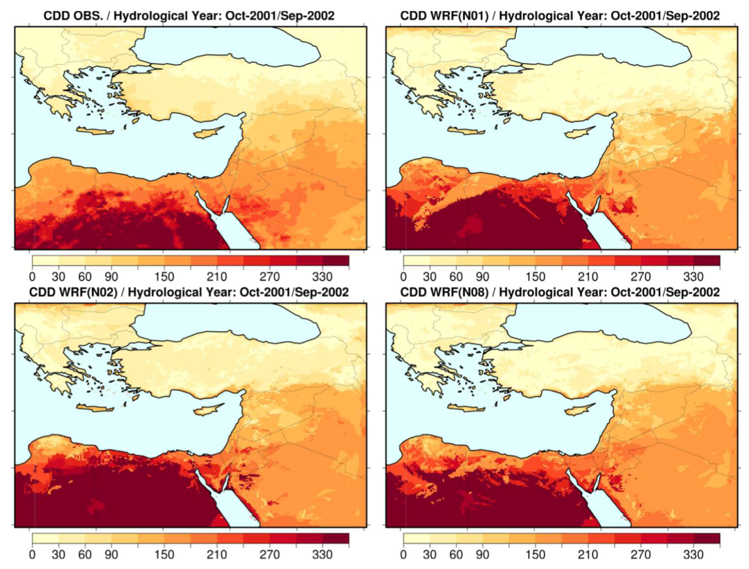
• Consecutive dry days (CDD): The greatest number of consecutive days with precipitation lower than 1 mm, within a year.
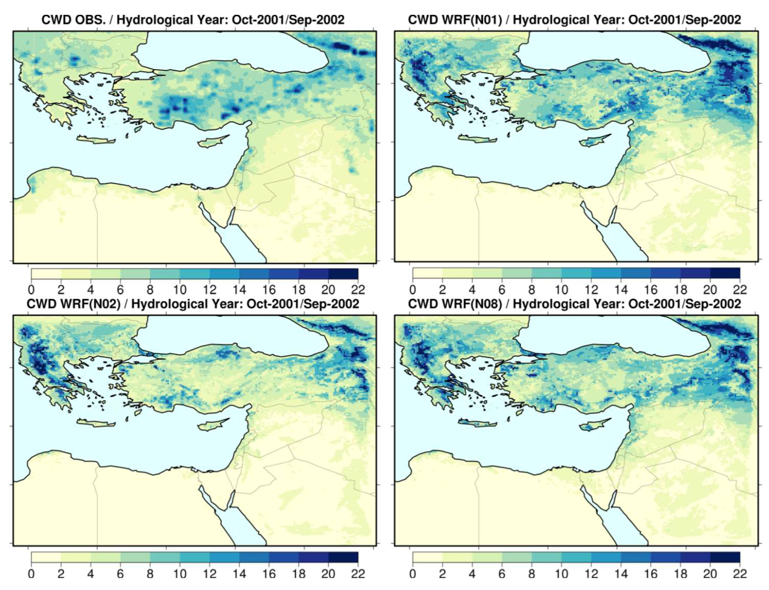
• Consecutive wet days (CWD): The greatest number of consecutive days with precipitation higher or equal to 1 mm, within a year.
• Annual count of rainy days (RR1): The annual count of days with observed rainfall greater than 1 mm.
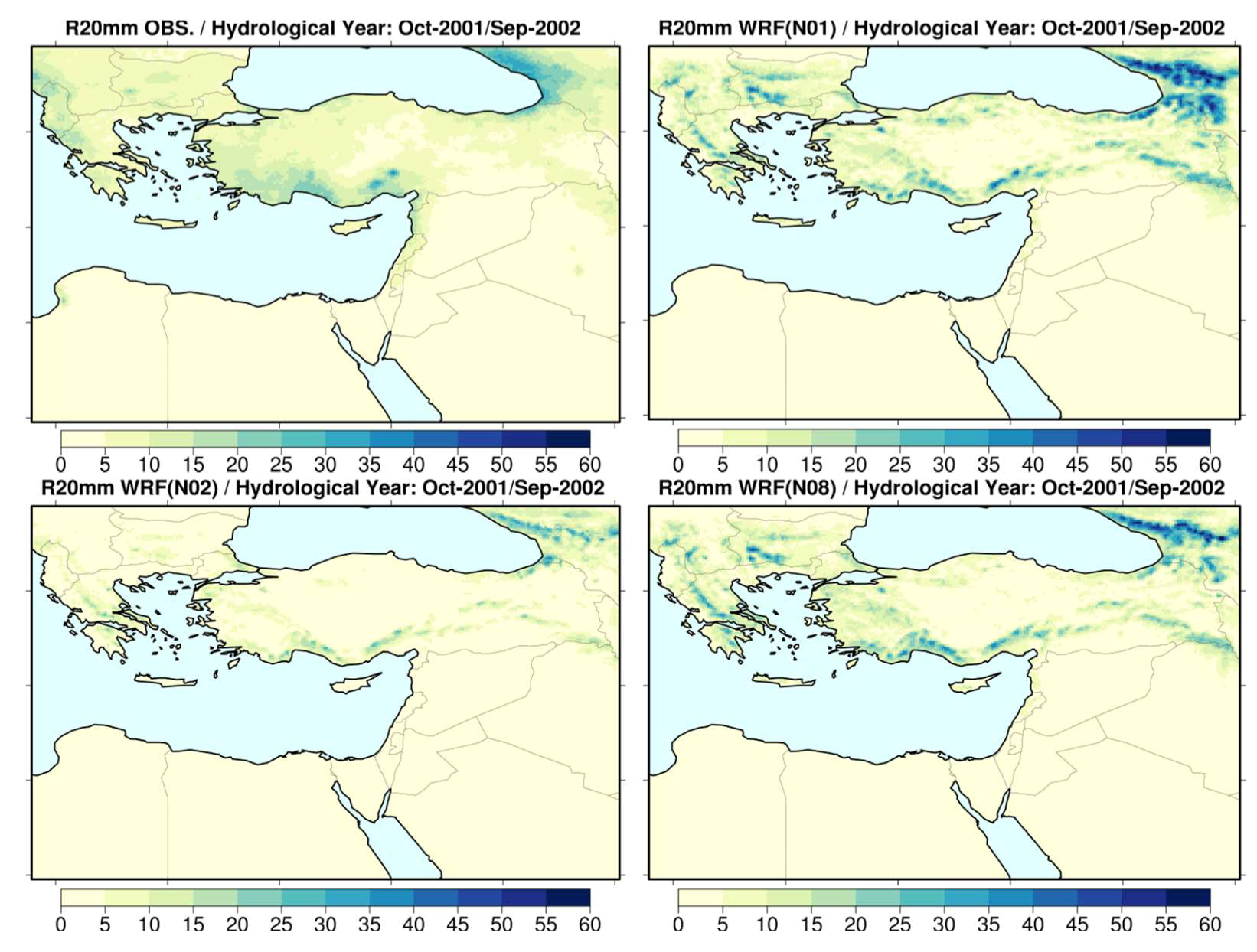
• Annual count of days with precipitation larger than 20 mm (R20).
• Highest five-day precipitation amount for each year (RX5D).
• Simple precipitation intensity index (SDII): Annual sum of precipitation during wet days (precipitation > 1 mm) divided by the annual count of wet days.

The threshold for a rainy day was set to 1 mm. The selection of a smaller threshold (e.g., 0.1 mm), which is sometimes used, would have likely affected some of the results, particularly the calculation of dry and wet spells, while this low rain intensity is insignificant in view of the regional hydrology in which we were interested. Such an occurrence of a near 0.1-mm rainy day could either break some of the dry spells or would result in a larger number of consecutive wet days, while the actual precipitation of that particular day is negligible and without any practical significance. Moreover, such an overestimation of the number of wet days per year would also affect the SDII and RR1 indices.

2.5. Statistical Metrics

The model skill in simulating precipitation and the effect of the tested nudging options was complementarily assessed by the calculation of four statistical metrics. For the first three metrics, this analysis was performed between the ensemble mean of gridded monthly observations (OBS) and WRF simulations (SIM), while it was summarized for the four rainfall regimes introduced in the previous paragraph. The fourth metric (threat score), which involves a more spatial comparison, was applied on observed and modeled annual precipitation sums. The four metrics are defined as follows:

• Spearman’s correlation coefficient (COR) was applied on the ranked monthly time series [36]:

  $$COR=\frac{cov\left(OBS,SIM\right)}{{\sigma }_{OBS}·{\sigma }_{SIM}}=\frac{{{\displaystyle \sum }}_{i=1}^n((OB{S}_i-\overline{OBS})\left(SI{M}_i-\overline{SIM}\right))}{{\sigma }_{OBS}·{\sigma }_{SIM}}$$

  (1)

  where n is the number of the sample, cov is covariance, and σ is the standard deviation. Significance of the correlations was assessed by the application of a t-test at the 95% significance level.
• The mean absolute error (MAE) was used to describe the average model performance error [37]:

  $$MAE=\frac{1}{n}{\displaystyle \sum }_{i=1}^n|SI{M}_i-OB{S}_i|$$

  (2)
• The modified index of agreement (MIA) was used as a standardized measure of the degree of the model prediction error [38,39]. This index varies between 0 and 1, with higher values indicating better agreement between the model and observations. It was introduced by Willmott [38] and refined by Legates and McCabe [39]:

  $$MIA=1-\frac{{{\displaystyle \sum }}_{i=1}^n|(OB{S}_i-SI{M}_i)|}{{{\displaystyle \sum }}_{i=1}^n|SI{M}_i-\overline{OBS}|+|OB{S}_i-\overline{OBS}|}$$

  (3)
• The threat score (TS) was used to measure the skill of predicting the area of precipitation for a certain threshold [8]. For this study, it was applied for the thresholds that defined each precipitation class in Section 2.4:

  $$TS=\frac{H}{\left(P+O-H\right)}$$

  (4)

  where P is the number of grid points in which the threshold amount of precipitation was simulated, O is the number of grid points in which the threshold amount was observed, and H is the number of grid points for which threshold precipitation was both simulated and observed. Values closer to 1 indicated a better agreement with the observations.

3. Results

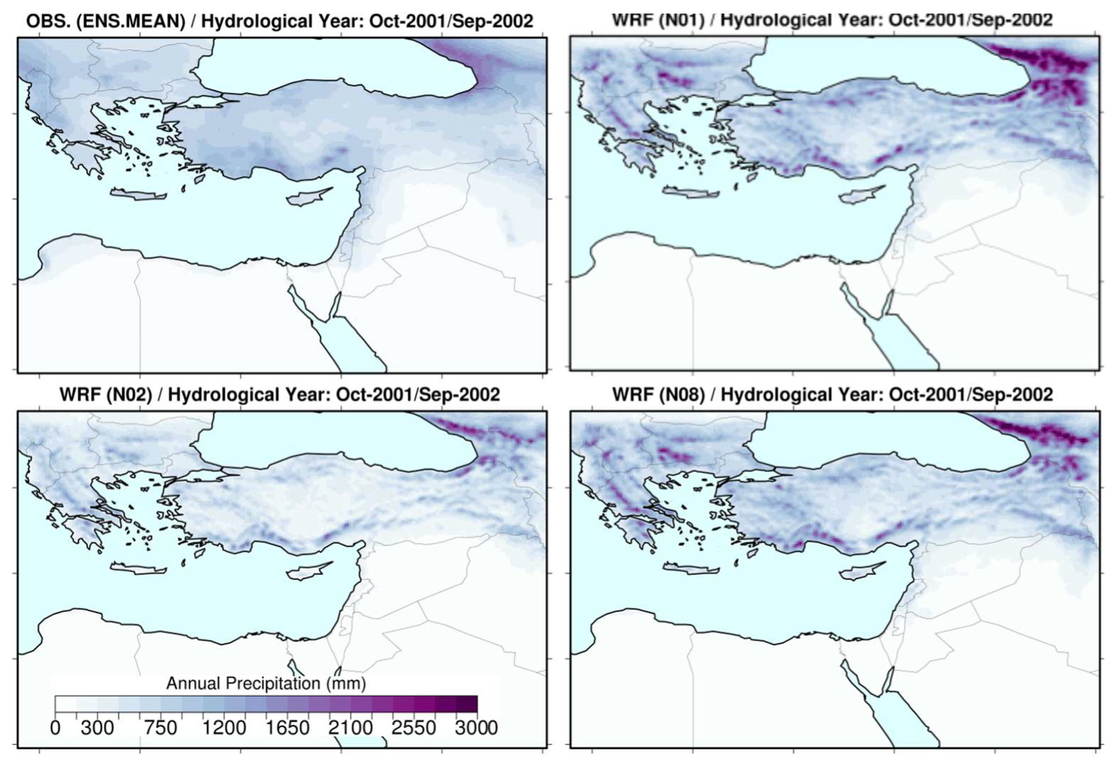
3.1. Annual Precipitation

Annual precipitation amounts for the hydrological year October 2001–September 2002 are presented in Figure 2 for both observations and WRF simulations. The ensemble mean of gridded observations (CHIRPS, CRU, E-OBS, and TRMM) suggests two very distinctive regimes: a very dry one in the southern half and a much wetter northern part of the EMME region. Over the eastern coast of the Black Sea and the Caucasus Mountains, annual rainfall is near 2500 mm.

The WRF simulations reproduced the overall precipitation distribution of this particular year (Figure 2). Nevertheless, the level of agreement with the observed conditions strongly varied over the different subregions. The no-nudged simulation (WRF-01) was in close agreement with the observations for the dry part of the domain. However, it generated more precipitation (up to 3000 mm/year) in the very wet regions of southern Turkey, the Caucasus Mountains, and the Balkans. The default grid nudging simulation (WRF-02) was generally drier and in closer agreement with the observations over the aforementioned regions. Our default spectral nudging simulation lay somewhere in between, representing more accurately precipitation over parts of the Balkan Peninsula, central Turkey, and Levantine coasts; however, it was still wetter than the ensemble mean of observations over the very wet regions. Compared to the default grid nudging (WRF-02), the default spectral option (WRF-08) was relatively wetter, probably due to the fact that the water vapor mixing ratio of the drier ERA-I driving data was not included in the variables to be nudged.

Individual plots for each observational dataset (in their original grids) and each WRF simulation are provided in Figure S2 of the Supplementary Materials. For parts of the region of interest, gridded observations can substantially differ, a fact that is mostly related to the raw meteorological information considered and not to their resolution [19]. Since we cannot objectively suggest which dataset is really the best throughout the domain, we hereafter focus our discussion mainly on the ensemble mean of the gridded observations.

Table 4. Observed annual precipitation total (in mm/year) and biases of the ERA-I reanalyses and each Weather Research and Forecasting (WRF) simulation, averaged over four rainfall regimes (Class 1: 0–100 mm/year, Class 2: 100–500 mm/year, Class 3: 500–1000 mm/year, Class 4: greater than 1000 mm/year). The percent coverage of grid points for each precipitation class over the Eastern Mediterranean domain is indicated. The lowest model biases (i.e., best performing simulations) are highlighted in bold.

	OBS	ERA-I	WRF01	WRF02	WRF03	WRF04	WRF05	WRF06	WRF07	WRF08	WRF09	WRF10
Class 1 (43.9%)	36	−9	−11	−23	−14	−28	−13	−19	−21	−11	−18	12
Class 2 (16.5%)	298	−6	−147	−233	−177	−233	−166	−223	−229	−155	−161	−159
Class 3 (33.6%)	710	−64	162	−230	50	−334	61	−161	−193	64	−16	40
Class 4 (5.9%)	1242	−293	386	249	161	−445	209	−104	−194	155	9	134

summarizes the observed annual precipitation amounts, as averages over the four rainfall regimes described in Section 2.4 and based on the ensemble mean of four observational datasets. Biases for each of the 10 WRF experiments are also indicated. We additionally present the same biases for the ERA-I reanalyses in order to explore any added value introduced by the higher-resolution WRF simulations. Overall, the ERA-I data underestimated rainfall over the very dry regime by 9 mm/year or 25% of the annual amount, while for Classes 2 and 3, they represented the observed rainfall reasonably well (negative biases below 10%). Nevertheless, they tended to be about 300 mm/year or 25% drier than observations for the very wet Class 4. Regarding WRF simulations, for the dry regions (Classes 1 and 2), none of the nudging options towards ERA-I (WRF-02–WRF-10) added value. In general, most nudging options, apart from the two no-PBL spectral ones (WRF-08 and WRF-10), showed a dry tendency (up to −80%) compared to the observations and the no-nudge WRF-01 simulation. Applying interior constraint methods within the PBL (WRF-04) resulted in a much drier and less realistic simulation. Configuration WRF-05, where only wind components and temperature were nudged, stood somewhere between simulations WRF-01 (no nudging) and WRF-03 (weak nudging). The sensitivity to the frequency of application of interior constraint towards ERA-I was assessed in experiments WRF-06 and WRF-07. For both cases, precipitation patterns were very similar to the default nudging; however, the model was less strongly constrained and generated slightly higher rainfall amounts. For the wet and very wet regions (Classes 3 and 4), some nudging options substantially improved the simulation of rainfall that was overestimated in the no-nudge case (WRF-01). Such an option is simulation WRF-09 (spectral nudging including the PBL), which introduced near-zero biases of annual precipitation total on average.

Besides some small differences, similar general conclusions can be drawn from a comparison between the WRF simulations and each observational dataset individually (Table S1 of the Supplementary Materials). This comparison highlights the consistently good performance of nudging simulations when specific humidity was not nudged (e.g., simulations WRF-05, WRF-08, WRF-09, and WRF-10). In addition, strong deviations from most observational datasets were evident when there was a strong specific humidity nudging (case WRF-02) or when grid nudging was applied within the PBL (WRF-04).

A possible explanation for why the nudged simulations tended to be drier than the reference simulation (WRF-01) over the Middle East and North African part of the domain is a general underestimation of the precipitable water within the atmospheric column for the ERA-I. In Figure 3, we present a comparison between the reanalysis data used to drive WRF and the radiosonde/satellite-based NVAP-M data. This is indicatively shown as an average for some the rainiest months of the study period (December 2001–March 2002). For the northern EMME domain, ERA-I data were in agreement with NVAP-M observations. Conversely, for parts of the Mediterranean Sea and extended land areas in Africa and Middle East, the ERA-I total column precipitable water (TCPW) was much lower than the observed values. Thus, any nudging for the specific humidity variable would likely introduce a drier atmospheric column in the WRF simulations. This inaccurate representation of humidity in the atmosphere by ERA-I, for parts of the domain, is likely to affect some of the nudging experiments and may introduce good results for the wrong reasons.

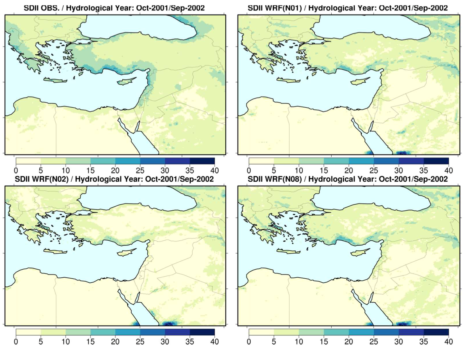
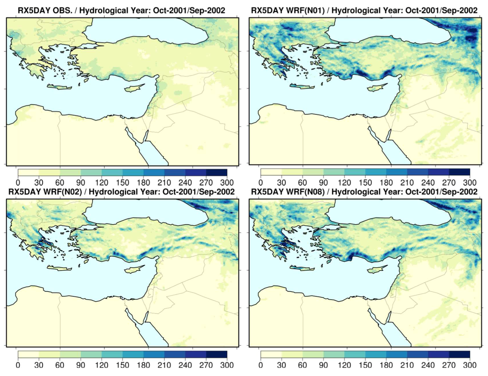
3.2. Precipitation Characteristics and Indices

The ability of WRF to represent several aspects of extreme rainfall is presented in this section through six widely used indices. The summary of the comparison with observations over the whole domain, for all experiments and each of the four precipitation regimes is presented in

Table 5. Observed values for six rainfall indices and biases for each WRF simulation, averaged over four precipitation regimes (Class 1: 0–100 mm/year, Class 2: 100–500 mm/year, Class 3: 500–1000 mm/year, Class 4: greater than 1000 mm/year). (CDD: Consecutive dry days, CWD: Consecutive wet days, RR1: Annual count of rainy days, R20: Annual count of days with precipitation larger than 20 mm, RX5D: Highest five-day precipitation amount for one year, SDII: Simple precipitation intensity index). The lowest model biases are highlighted in bold.

		OBS	WRF01	WRF02	WRF03	WRF04	WRF05	WRF06	WRF07	WRF08	WRF09	WRF10
CDD	Class 1	225.5	13.4	33.3	24.4	51.4	20.4	23.8	30.8	18.6	27.5	21.0
	Class 2	129.9	4.8	22.3	14.1	46.7	13.4	11.7	19.2	20.0	22.1	21.8
	Class 3	51.9	−18.7	−4.4	−14.2	9.1	−15.4	−4.2	−5.5	−13.0	−10.5	−11.3
	Class 4	33.4	−11.6	−3.0	−9.0	5.1	−9.6	−4.6	−4.5	−7.8	−7.9	−6.8
CWD	Class 1	1.5	−0.1	−0.4	−0.2	−0.7	−0.2	−0.2	−0.4	−0.1	−0.3	−0.2
	Class 2	4.6	−0.7	−1.9	−1.1	−2.3	−0.9	−1.4	−1.8	−0.7	−0.9	−0.7
	Class 3	6.7	2.5	0.5	1.7	−1.7	1.7	2.1	1.1	2.0	1.3	1.7
	Class 4	9.7	3.6	1.2	2.6	−3.0	3.2	3.2	1.8	2.6	1.2	2.1
RR1	Class 1	7.2	−1.9	−3.8	−2.6	−5.4	−2.2	−3.0	−3.5	−2.1	−3.3	−2.3
	Class 2	38.1	−9.9	−22.5	−14.3	−25.3	−12.2	−19.9	−21.9	−11.5	−12.9	−11.9
	Class 3	79.3	31.6	4.8	24.2	−22.5	25.8	15.6	10.5	24.4	16.3	21.0
	Class 4	113.9	35.8	8.7	25.3	−24.8	28.0	19.3	13.3	23.4	17.7	20.6
R20	Class 1	0.1	0.0	−0.1	0.0	−0.1	0.0	−0.1	−0.1	0.0	0.0	0.0
	Class 2	2.7	−1.9	−2.5	−2.1	−2.4	−2.1	−2.5	−2.5	−2.0	−2.0	−2.0
	Class 3	7.9	0.7	−4.8	−1.0	−5.0	−1.1	−4.4	−4.6	−0.8	−1.7	−0.9
	Class 4	17.7	4.5	−7.6	0.3	−8.2	0.7	−5.5	−6.8	0.4	−2.0	0.1
SDII	Class 1	3.9	−1.1	−1.9	−1.3	−1.8	−1.4	−1.8	−1.9	−1.2	−1.3	−1.1
	Class 2	7.4	−3.0	−4.2	−3.3	−3.5	−3.3	−4.1	−4.1	−2.9	−3.0	−3.0
	Class 3	9.6	−1.9	−4.1	−2.5	−3.2	−2.5	−4.0	−4.1	−2.3	−2.5	−2.3
	Class 4	12.7	−2.1	−4.8	−2.8	−3.9	−2.7	−4.4	−4.7	−2.6	−3.3	−2.6
RX5D	Class 1	9	1.3	−3.3	0.6	−4.3	0.4	−1.8	−2.8	1.2	−0.6	1.1
	Class 2	35.8	−4.8	−19.5	−8.3	−16.5	−8.9	−17.6	−18.6	−4.7	−6.5	−5.9
	Class 3	51.3	44.9	10.5	35.6	8.7	33.3	14.1	12.0	34.8	28.8	34.6
	Class 4	74.1	87.4	30.8	64.1	25.5	60.7	43.0	33.2	60.1	47.2	60.5

. Relevant maps for the whole domain are presented only for the ensemble mean of the daily datasets (CHIRPS, TRMM, and E-OBS) and simulations WRF-01, WRF-02, and WRF-08 (i.e., no-nudging, default grid nudging, and default spectral nudging, respectively). These maps are only presented over land grid points in order to facilitate the comparison between observations and simulations.

The maximum number of consecutive dry days is presented in Figure 4. According to observations, this number ranged from more than 300 for the hyperarid regions of the Middle East and North Africa up to less than 30 days in the much wetter northern part of the domain. In general, WRF was able to well reproduce the spatial patterns of CDD index. The summary of Table 5 indicates that, on one hand, the no-nudge simulation (WRF-01) was closer to the observations’ ensemble mean for the dry regimes (Classes 1 and 2). On the other hand, it underestimated the maximum length of dry spells for the two wetter classes (3 and 4). According to Table 5, this underestimation of the CDD index was also evident for the three spectral nudging cases (WRF-08–WRF-10). Most of the grid nudging options showed some added value in the simulation of extreme dry spells for the wet regimes.

The maximum length of wet spells per year, also known as the consecutive wet days index (CWD), is presented in Figure 5. As expected, according to the gridded observations, this index had very low values (<5 days) for the southern part of the domain. On the contrary, wet spells of maximum duration of more than 20 days were observed over the wettest parts of the domain. Model simulations with WRF generally tended to agree with the observed data. As seen in Table 5, the no-nudge (WRF-01) and spectral nudging simulations (WRF-08-WRF-10) were better in representing CWD for the dry regimes, while on the other hand, some grid analysis nudging options (e.g., WRF-02) outperformed the others for the wetter precipitation regimes. This is also evident from the maps of Figure 5.

The annual count of rainy days (RR1 index) for the investigated hydrological year is presented in Figure 6. According to the observations, there was a strong north–south gradient from more than 150 rainy days per year in the north to less than 10 rainy days per year in the southern part of the domain. WRF realistically reproduced the number of rainy days for most of the Eastern Mediterranean. According to Table 5 and Figure 6, nudging on average tended to improve the simulation of RR1 for the two wet regimes. It underestimated this index for the dry regions, which were better represented by the no-nudge configuration. The improvements introduced for the wet regions were more evident in the default grid nudging simulation (WRF-02).

For the number of heavy precipitation days (>20 mm) per year, gridded observations suggest that over extended regions of western Greece, Albania, southern Turkey, and the Caucasus Mountains, there were more than 30 heavy precipitation days recorded during the period considered (Figure 7). The spatial pattern of this index was sufficiently well reproduced by the model simulations. As expected, for regions in the hyperarid precipitation class, all model configurations were found to be close to the observations, indicating near-zero days of heavy rainfall (Table 5). For grid points of the second precipitation regime (100–500 mm/year), all WRF simulations underestimated the occurrence of heavy precipitation days. For the very wet regime, some nudging options, including the weak grid nudging (WRF-03) and the spectral nudging options (WRF-08–WRF-10), outperformed the others.

SDII is a simple measure of precipitation intensity. In general, this index is larger over the coastal regions of the Eastern Mediterranean (Figure 8). Particularly over the west parts of Greece, the south coast of Turkey, and the east coast of Black Sea, the ensemble mean of gridded observations indicated an average of more than 25 mm per rainy day. According to Table 5, all WRF simulations generally tended to underestimate this index for all weather regimes, while nudging did not introduce any improvements. Nevertheless, the no-nudging simulation (WRF-02) and the spectral nudging ones (WRF-08–WRF-10) were closer to the observed values over the very wet regions.

Figure 9 depicts the most severe five-day events in terms of precipitation during the study period. Locally, up to 150–200 mm during a single five-day period were found, mainly in the high-elevation and coastal regions of the northern part of the domain. WRF simulations spatially reproduced the RX5DAY index. For the wet parts of the domain, grid nudging options better represented the values of this index, which were highly overestimated in the no-nudging and spectral nudging runs (Table 5).

3.3. Statistical Metrics

The performance of the 10 WRF simulations was additionally assessed through the calculation of statistical metrics that consider both biases of monthly precipitation amounts and temporal variability throughout the study period. These results are summarized in

Table 6. Statistical metrics (COR: correlation coefficient, MAE: mean absolute error (mm/mo), MIA: modified index of agreement, TS: threat score) between the observed monthly precipitation (ensemble mean of gridded data) and WRF simulations. Results are averaged for each precipitation class and for all grid points (average).

		WRF01	WRF02	WRF03	WRF04	WRF05	WRF06	WRF07	WRF08	WRF09	WRF10
COR	Class 1	0.50	0.49	0.52	0.56	0.48	0.4	0.47	0.52	0.52	0.53
	Class 2	0.81	0.76	0.83	0.76	0.82	0.72	0.75	0.84	0.84	0.84
	Class 3	0.71	0.71	0.74	0.76	0.73	0.65	0.68	0.76	0.78	0.77
	Class 4	0.56	0.56	0.55	0.55	0.55	0.5	0.56	0.56	0.56	0.56
MAE	Class 1	2.1	2.1	2.1	2.1	2.1	2.3	2.1	2.1	2.0	2.2
	Class 2	10.1	12.6	10.1	12.4	9.9	12.6	12.5	9.6	9.5	9.7
	Class 3	35.6	28.7	31.0	31.0	30.8	28.8	28.6	30.2	26.3	29.5
	Class 4	70.9	48.9	61.3	52.5	62.7	54.1	49.4	59.2	52.6	60.0
MIA	Class 1	0.43	0.31	0.39	0.22	0.42	0.32	0.31	0.42	0.37	0.41
	Class 2	0.58	0.35	0.54	0.34	0.56	0.37	0.36	0.6	0.58	0.59
	Class 3	0.59	0.52	0.6	0.48	0.61	0.52	0.52	0.62	0.64	0.62
	Class 4	0.54	0.49	0.53	0.44	0.52	0.48	0.49	0.53	0.53	0.52
TS	Class 1	0.79	0.64	0.75	0.52	0.8	0.68	0.63	0.78	0.77	0.77
	Class 2	0.37	0.08	0.29	0.08	0.31	0.11	0.1	0.35	0.29	0.31
	Class 3	0.55	0.36	0.57	0.18	0.57	0.45	0.41	0.59	0.61	0.58
	Class 4	0.28	0.38	0.33	0.23	0.33	0.43	0.4	0.33	0.38	0.33

as averages over the four rainfall regimes. The best values for each metric are highlighted in bold. The statistical analysis indicated lower correlation coefficient values for the extreme low and high precipitation regimes (Classes 1 and 4). For the arid Class 1, although the reference no-nudge simulation was in closer agreement to the gridded observations for the annual precipitation sums, some nudging options added value in terms of covariance and thus correlation with the monthly observations. Nevertheless, on average, these correlations were not statistically significant (for a 95% confidence interval). For the wetter regimes (Classes 2–4), the added value in the nudging simulations was more evident and correlations coefficients were significant, while the spectral nudging options outperformed the other in terms of this metric.

As expected, mean absolute error values were lower for the arid regimes. For such cases, the differences between WRF simulations were smaller since precipitation occurred in short wet periods throughout the year. As a result, MAE values, based on monthly precipitation, were smoothed since, for the long dry periods of the year, the model was for all runs in good agreement with the observations. Such examples are the Benghazi and Athalassa stations presented in Figure 10. For the wetter regimes of Classes 3 and 4, the improvements in MAE values were stronger.

On average, the modified index of agreement between observations and WRF simulations was also lower for the hyperarid regions, indicating a lower model skill for this type of weather regime. However, most simulations that did not nudge specific humidity (WRF-01, WRF-05, WRF-08, WRF-09, and WRF-10) performed similarly and were in closer agreement with the observations.

The threat score summarizes for each simulation the total area that coincides with the observations for each rainfall class (Table 6). Consistent with the MIA scores, the no-nudge and spectral nudging options outperformed the others for the drier classes. On the other hand, there was some added value for several grid (and spectral) nudging options for the rainy regimes, which was more evident for the very wet Class 4.

3.4. Monthly Precipitation at Stations

Although it is not entirely consistent to directly compare area averages, such as model grids, with point measurements, especially for regions affected by local convective rainfall, a complementary monthly comparison between station data, gridded observations, and simulations is presented in Figure 10 for six station locations. This is given in the form of monthly precipitation values, as the averaging is expected to smooth some of the local variability. The vertical bars of Figure 10 indicate the range between the four gridded observations (CRU, CHIRPS, E-OBS, and TRMM) at the nearest grid point for each location. For most cases, the range between the different observational sources was high during wet months; however, their ensemble mean was usually in good agreement with the station measurements. Interestingly, for some locations, the spread between the gridded observations over the wet months of the year was comparable or larger than the spread of the simulations. Such examples include December precipitation in Benghazi and Diyiarbakir and during January in Zefat, highlighting issues of observational uncertainty in the region of interest [19].

Most WRF experiments simulated precipitation well during the dry summer and early autumn months, while the effect of nudging during this period of the year was minimal. Nevertheless, for the rest of the year the simulations differed with varying skills. For the location of Benghazi in Libya, which is adjacent to the western boundary of the simulation domain, all WRF simulations failed in reproducing the observed rainfall for the wet period of the year. On the other hand, for the station of Larissa in central Greece, the model performed fairly well throughout the hydrological year 2001–2002. Several grid nudging options improved the monthly distribution of rainfall compared to the no-nudge case (solid black line), which overestimated measured rainfall. A clear improvement was also seen for the Athalassa station in the outskirts of Nicosia in Cyprus. In this case, precipitation improved (compared to the no-nudge experiment), especially when spectral nudging techniques were applied (Figure 10). For the Alanya station in southern Turkey and Zefat in the northern highlands of Israel (Figure 10—top left and bottom left panels respectively), all WRF simulations significantly underestimated rainfall during the winter and spring months. This is likely related to inconsistencies between real station elevation and the model’s representation in these 12-km resolution simulations (Table 3). Nevertheless, spectral nudging slightly improved the modeled rainfall. For Diyarbakir station in southeast Turkey (Figure 10 middle left) in the winter months, some nudging options negatively affected precipitation, while others, including the spectral ones, were as good as the no-nudge experiment. This was not the case for the transitional spring season, where some grid nudging options improved the simulation of precipitation. One such case was simulation WRF-05, where all variables were nudged except specific humidity.

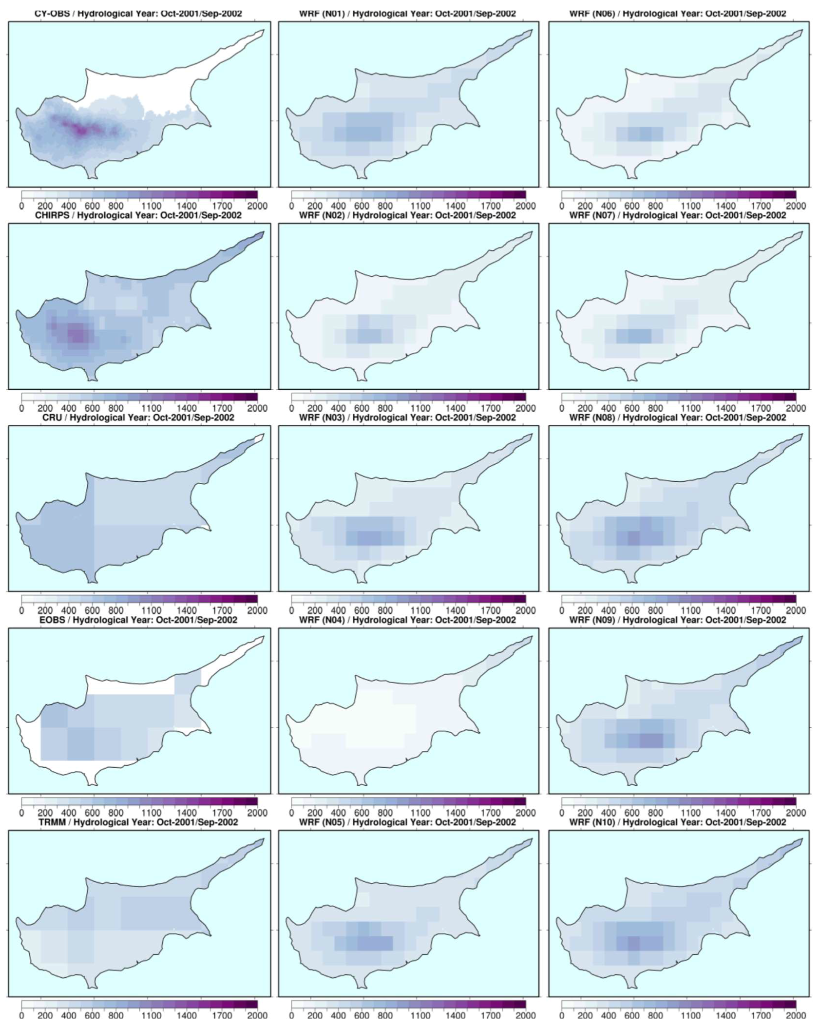
3.5. The Case of Cyprus

A more regionalized comparison based on high-quality and high-resolution data for the island of Cyprus is presented in this section. The left panels of Figure 11 refer to five observation-based datasets and the precipitation total of the hydrological year 2001–2002. It was assumed that the most accurate representation of rainfall was provided by the local CY-OBS dataset, which is an optimized spatial interpolation of 145 daily rain gauges [35]. Interestingly, only the 5-km CHIRPS dataset could approximately capture the precipitation gradients over Cyprus. Precipitation was influenced by the presence of the Troodos Mountains, located towards the central/southwest part of the island. Due to orographic effects, rainfall maxima of up to 1400 mm/year were found at the higher-elevation regions for the particular year. On the other hand, minimum annual values of the range of 300 mm/year were found in the central plain and eastern parts of Cyprus as a result of the “rain shadow” effect, considering that most cyclonic systems approach the region from the west. All other datasets (CRU, E-OBS, and TRMM), which were of much coarser horizontal resolution, strongly underestimated precipitation, and they also misrepresented the spatial distribution throughout the island. This is also the case for the ERA-I reanalyses, which were used as driving data for the WRF simulations (not shown).

The WRF model simulations for Cyprus (presented only over land points) are depicted in the middle and right panels of Figure 11. All simulations, except WRF-04, could capture the annual rainfall peaks over the Troodos Mountains. Nevertheless, there was some disagreement in the simulated precipitation amounts. For this local-scale comparison, the most accurate representation of rainfall was found for the no-nudge (WRF-01) and the three spectral-nudging simulations (WRF-08–WRF-10), which did not include humidity as a nudging variable. As discussed above, this can be attributed to the fact that the ERA-I driving data underestimated moisture in the atmosphere over the easternmost part of the Mediterranean. The TCPW maps of Figure 3 support this argument. Over Cyprus, the ERA-I monthly mean TCPW was higher than the NVAP-M satellite data, because in the ERA-I simulations, Cyprus was not resolved as land and was considered a sea grid point. However, over the surrounding Mediterranean Sea and the adjacent land to the south and east, ERA-I tended to underestimate TCPW during most months of the rainy season, which resulted in reduced precipitation locally for the strongly nudged simulations. We underscore the importance of investigating the quality and accuracy of boundary conditions (reanalysis or global model simulations) before applying any downscaling or nudging methods. In a previous study for the same region, WRF showed the potential for improved simulation of precipitation by convection-permitting simulations at higher horizontal resolution [23]. Nevertheless, at least for the moment, application of such configurations for long climate runs is not realistic considering the computational resources and data storage involved.

3.6. Computational Cost

The application of nudging techniques implies additional computational cost. When it comes to long-term forecast or future climate simulations of decadal scales, this additional cost should be considered during the design of such downscaling experiments. Our default no-nudging simulation of 13 months (1 year plus 1 month of spin-up) on 120 CPU processors of the Cy-Tera High Performance Facilities of The Cyprus Institute (http://web.cytera.cyi.ac.cy/) required about 22 h to be completed. The grid nudging options (WRF-02–WRF-05) added an additional 15% to this time. Simulations WRF-06 and WRF-07, where nudging was not applied every 6 h, were less comprehensive, as they only introduced an additional cost of about +8%. We found that the costliest option in WRF was with spectral nudging. It added an additional computational load of 50–60%. Therefore, this option might not be optimal for long runs, although it improved several aspects of mean and extreme precipitation, particularly for the wet regimes of the region of interest. These estimations are valid only for the current WRF configuration in terms of horizontal/vertical resolution and parameterization schemes used. We note that some additional cost, regarding the preparation of the nudging files from the WRF prior to the simulations, was not included in these estimations. Regarding other modeling systems, Alexandru et al. [3] suggested that simulation time in their Canadian RCM experiments was extended by no more than 5% when spectral nudging was applied. Therefore, they concluded that computational resources should not be the main consideration regarding the use of nudging in a specific project.

4. Discussion and Conclusions

We investigated the sensitivity of various hydroclimatic variables to different interior nudging options applied in the WRF model for the EMME region. In general, the reference WRF physics configuration spatially reproduced precipitation patterns over the study region. Nevertheless, the model tended to underestimate rainfall over relatively dry regions (between −30% and −50% of the annual totals), while on the other hand, it had a positive bias (+30%) over the wet and very wet regimes. Nudging had a significant effect on the WRF simulations. Both grid and spectral nudging resulted in drying, which was most pronounced for grid nudging. In particular, nudging reduced the overestimation of rainfall over wet regions because the ERA-I atmospheric column was locally found to be drier compared to observations. However, this enhanced the underestimation of rainfall in drier regions. Similar to mean precipitation, nudging towards ERA-I affected several rainfall characteristics through improvements of most precipitation indices in wet regimes and worsening in dry regions. An exception was the simple precipitation intensity index, for which no improvement was achieved. In agreement with the relevant literature, nudging of specific humidity within the PBL made the simulations even drier, hence too dry, whereas spectral nudging with PBL still yielded acceptable results.

For many cases, such as for the annual totals over wet regimes, the spectral nudging of WRF was found to outperform non-nudging and grid nudging, introducing, however, a significant load in terms of computational cost. The additional cost of grid nudging was much smaller, indicating greater potential for use in long-term climate simulations. The better performance of spectral nudging can probably be attributed to the more accurate representation of synoptic meteorological conditions that generate precipitation, since geopotential height was also nudged for certain atmospheric disturbances. Moreover, the ERA-I errors in the estimation of the atmospheric column water vapor were not propagated in the regional simulations, since this variable was not nudged when the spectral nudging option was activated.

Since some nudging options were found to substantially improve the WRF simulations for particular locations, especially for the length of wet/dry spells (CWD and CDD indices), mean, and extreme rainfall (RR1, RX5D, and R20 indices) in wet environments, the application of statistically based bias correction methods in such cases could eventually be limited or omitted. This is of great importance for the use of atmospheric model output as input for impact studies (e.g., hydrological, agro-ecological, vector borne disease spreading, etc.), since the latter ones are very sensitive to absolute thresholds of concurrent temperature and precipitation in daily or subdaily time scales. The concurrency in the values of meteorological variables can be suppressed when bias correction is independently applied for temperature and precipitation.

Considering all results, after ensuring that the global forcing data (e.g., reanalyses) are of high quality over the specific region of interest, we recommend that a weak grid nudging can improve several aspects of rainfall, reduce some biases, and add value to regional climate simulations without adding a significant computational load. Similar conclusions were presented in previous studies [8,16]. These studies highlighted that the application of interior nudging in regional climate simulations increased the skill of RCMs to reproduce mean climatic conditions and also extremes.

Further work should be conducted regarding the effect of nudging towards global climate models for past and future projections. Another aspect not investigated in this study is the effect of nudging when multiple nesting domains are used. Nevertheless, for the region of interest and for further downscaling, this type of 12-km output can be considered as better LBCs compared to the original ERA-I data. This can be particularly relevant for similar WRF studies and contributions to the CORDEX initiative. Interior nudging could potentially add value for large domains such as the MENA-CORDEX or CORDEX-AFRICA. The further increase of horizontal resolution is expected to improve modeled precipitation through the more realistic representation of orography and the explicit treatment of convective processes [23,40,41]. Finally, although nudging can be considered as a “tuning” method and does not directly improve the physics of the models, it can still be a very efficient tool for impact and adaptation studies, especially when systematic model biases are corrected. However, the further development and improvement of weather/climate models in terms of representation of physical processes should remain a priority.

References

1. Lucas-Picher, P.; Cattiaux, J.; Bougie, A.; Laprise, R. How does large-scale nudging in a regional climate model contribute to improving the simulation of weather regimes and seasonal extremes over North America? Clim. Dyn. 2016, 46, 929–948. [Google Scholar] [CrossRef]
2. Liu, P.; Tsimpidi, A.P.; Hu, Y.; Stone, B.; Russell, A.G.; Nenes, A. Differences between downscaling with spectral and grid nudging using WRF. Atmos. Chem. Phys. 2012, 12, 3601–3610. [Google Scholar] [CrossRef] [Green Version]
3. Alexandru, A.; de Elia, R.; Laprise, R.; Separovic, L.; Biner, S. Sensitivity study of regional climate model simulations to Large-Scale nudging parameters. Mon. Weather Rev. 2009, 137, 1666–1686. [Google Scholar] [CrossRef]
4. Spero, T.L.; Otte, M.J.; Bowden, J.H.; Nolte, C.G. Improving the representation of clouds, radiation, and precipitation using spectral nudging in the weather research and forecasting model. J. Geophys. Res. Atmos. 2014, 119, 11682–11694. [Google Scholar] [CrossRef]
5. Stauffer, D.R.; Seaman, N.L. Use of Four-Dimensional data assimilation in a Limited-Area mesoscale model. Part I: Experiments with Synoptic-Scale data. Mon. Weather Rev. 1990, 118, 1250–1277. [Google Scholar] [CrossRef]
6. Von Storch, H.; Langenberg, H.; Feser, F. A spectral nudging technique for dynamical downscaling purposes. Mon. Weather Rev. 2000, 128, 3664–3673. [Google Scholar] [CrossRef]
7. Omrani, H.; Drobinski, P.; Dubos, T. Optimal nudging strategies in regional climate modelling: Investigation in a Big-Brother experiment over the European and Mediterranean regions. Clim. Dyn. 2013, 41, 2451–2470. [Google Scholar] [CrossRef]
8. Lo, J.C.-F.; Yang, Z.-L.; Pielke, R.A., Sr. Assessment of three dynamical climate downscaling methods using the Weather Research and Forecasting (WRF) model. J. Geophys. Res. Atmos. 2008, 113, D09112. [Google Scholar] [CrossRef]
9. García-Díez, M.; Fernández, J.; Fita, L.; Yagüe, C. Seasonal dependence of WRF model biases and sensitivity to PBL schemes over Europe. Q. J. R. Meteorol. Soc. 2013, 139, 501–514. [Google Scholar] [CrossRef]
10. Arritt, R.W.; Rummukainen, M. Challenges in Regional-Scale climate modeling. Bull. Am. Meteorol. Soc. 2011, 92, 365–368. [Google Scholar] [CrossRef]
11. Bowden, J.H.; Otte, T.L.; Nolte, C.G.; Otte, M.J. Examining interior grid nudging techniques using Two-Way nesting in the WRF model for regional climate modeling. J. Clim. 2012, 25, 2805–2823. [Google Scholar] [CrossRef]
12. Miguez-Macho, G.; Stenchikov, G.L.; Robock, A. Spectral nudging to eliminate the effects of domain position and geometry in regional climate model simulations. J. Geophys. Res. Atmos. 2004, 109. [Google Scholar] [CrossRef] [Green Version]
13. Castro, C.L.; Pielke, R.A.; Leoncini, G. Dynamical downscaling: Assessment of value retained and added using the regional atmospheric modeling system (RAMS). J. Geophys. Res. 2005, 110. [Google Scholar] [CrossRef]
14. Deng, A.; Stauffer, D.R. On improving 4-km mesoscale model simulations. J. Appl. Meteorol. Climatol. 2006, 45, 361–381. [Google Scholar] [CrossRef]
15. Salathé, E.P.; Steed, R.; Mass, C.F.; Zahn, P.H. A High-Resolution climate model for the U.S. pacific northwest: Mesoscale feedbacks and local responses to climate change. J. Clim. 2008, 21, 5708–5726. [Google Scholar] [CrossRef]
16. Otte, T.L.; Nolte, C.G.; Otte, M.J.; Bowden, J.H. Does nudging squelch the extremes in regional climate modeling? J. Clim. 2012, 25, 7046–7066. [Google Scholar] [CrossRef]
17. Bullock, O.R.; Alapaty, K.; Herwehe, J.A.; Mallard, M.S.; Otte, T.L.; Gilliam, R.C.; Nolte, C.G. An Observation-Based investigation of nudging in WRF for downscaling surface climate information to 12-km grid spacing. J. Appl. Meteorol. Climatol. 2013, 53, 20–33. [Google Scholar] [CrossRef]
18. Lelieveld, J.; Proestos, Y.; Hadjinicolaou, P.; Tanarhte, M.; Tyrlis, E.; Zittis, G. Strongly increasing heat extremes in the Middle East and North Africa (MENA) in the 21st century. Clim. Chang. 2016, 137, 245–260. [Google Scholar] [CrossRef] [Green Version]
19. Zittis, G. Observed rainfall trends and precipitation uncertainty in the vicinity of the Mediterranean, Middle East and North Africa. Theor. Appl. Climatol. 2018, 134, 1207–1230. [Google Scholar] [CrossRef]
20. Skamarock, W.C.; Klemp, J.B.; Dudhia, J.; Gill, D.O.; Barker, D.M.; Duda, M.G.; Huang, X.-Y.; Wang, W.; Powers, J.G. A Description of the Advanced Research WRF Version 3; NCAR Technical Note, NCAR/TN-475+STR; National Center for Atmospheric Research: Boulder, CO, USA, 2008. [Google Scholar]
21. Simmons, A.; Uppala, S.; Dee, D.; Kobayashi, S. ERA-interim: New ECMWF reanalysis products from 1989 onwards. ECMWF Newsl. 2007, 110, 26–35. [Google Scholar] [CrossRef]
22. Zittis, G.; Hadjinicolaou, P.; Lelieveld, J. Comparison of WRF model physics parameterizations over the MENA-CORDEX domain. Am. J. Clim. Chang. 2014, 3, 490–511. [Google Scholar] [CrossRef]
23. Zittis, G.; Bruggeman, A.; Camera, C.; Hadjinicolaou, P.; Lelieveld, J. The added value of convection permitting simulations of extreme precipitation events over the eastern Mediterranean. Atmos. Res. 2017, 191, 20–33. [Google Scholar] [CrossRef]
24. Zittis, G.; Hadjinicolaou, P. The effect of radiation parameterization schemes on surface temperature in regional climate simulations over the MENA-CORDEX domain. Int. J. Climatol. 2017, 37, 3847–3862. [Google Scholar] [CrossRef]
25. Janjić, Z.I. The Step-Mountain eta coordinate model: Further developments of the convection, viscous sublayer, and turbulence closure schemes. Mon. Weather Rev. 1994, 122, 927–945. [Google Scholar] [CrossRef]
26. National Oceanic and Atmospheric Administration (NOAA). Changes to the NCEP Meso Eta Analysis and Forecast System: Increase in Resolution, New Cloud Microphysics, Modified Precipitation Assimilation, Modified 3DVAR Analysis. Available online: http://etamodel.cptec.inpe.br/documentation/ (accessed on 29 November 2018).
27. Iacono, M.J.; Delamere, J.S.; Mlawer, E.J.; Shephard, M.W.; Clough, S.A.; Collins, W.D. Radiative forcing by long-lived greenhouse gases: Calculations with the AER radiative transfer models. J. Geophys. Res. Atmos. 2008, 113. [Google Scholar] [CrossRef] [Green Version]
28. Tewari, M.; Chen, F.; Wang, W.; Dudhia, J.; LeMone, M.A.; Mitchell, K.; Ek, M.; Gayno, G.; Wegiel, J.; Cuenca, R.H. Implementation and verification of the unified NOAH land surface model in the WRF model. In Proceedings of the 20th Conference on Weather Analysis and Forecasting/16th Conference on Numerical Weather Prediction, Seattle, WA, USA, 12–16 January 2004. [Google Scholar]
29. Maraun, D.; Widmann, M.; Gutiérrez, J.M.; Kotlarski, S.; Chandler, R.E.; Hertig, E.; Wibig, J.; Huth, R.; Wilcke, R.A.I. VALUE: A framework to validate downscaling approaches for climate change studies. Earths Future 2015, 3, 1–14. [Google Scholar] [CrossRef] [Green Version]
30. Vonder Haar, T.H.; Bytheway, J.L.; Forsythe, J.M. Weather and climate analyses using improved global water vapor observations. Geophys. Res. Lett. 2012, 39. [Google Scholar] [CrossRef] [Green Version]
31. Harris, I.; Jones, P.D.; Osborn, T.J.; Lister, D.H. Updated high-resolution grids of monthly climatic observations—The CRU TS3.10 dataset. Int. J. Climatol. 2014, 34, 623–642. [Google Scholar] [CrossRef] [Green Version]
32. Funk, C.; Peterson, P.; Landsfeld, M.; Pedreros, D.; Verdin, J.; Shukla, S.; Husak, G.; Rowland, J.; Harrison, L.; Hoell, A.; et al. The climate hazards infrared precipitation with stations—A new environmental record for monitoring extremes. Sci. Data 2015, 2, 150066. [Google Scholar] [CrossRef] [PubMed]
33. Haylock, M.R.; Hofstra, N.; Klein Tank, A.M.G.; Klok, E.J.; Jones, P.D.; New, M. A European daily high-resolution gridded dataset of surface temperature and precipitation. J. Geophys. Res. Atmos. 2008, 113, D20119. [Google Scholar] [CrossRef]
34. Huffman, G.J.; Adler, R.F.; Bolvin, D.T.; Gu, G.; Nelkin, E.J.; Bowman, K.P.; Hong, Y.; Stocker, E.F.; Wolff, D.B. The TRMM Multi-Satellite Precipitation Analysis: Quasi-Global, Multi-Year, Combined-Sensor Precipitation Estimates at Fine Scale. J. Hydrometeorol. 2007, 8, 38–55. [Google Scholar] [CrossRef]
35. Camera, C.; Bruggeman, A.; Hadjinicolaou, P.; Pashiardis, S.; Lange, M.A. Evaluation of interpolation techniques for the creation of gridded daily precipitation (1 × 1 km2); Cyprus, 1980–2010. J. Geophys. Res. Atmos. 2014, 119, 693–712. [Google Scholar] [CrossRef]
36. Spearman, C. The proof and measurement of correlation between two things. Am. J. Psychol. 1904, 15, 72–101. [Google Scholar] [CrossRef]
37. Willmott, C.J.; Matsuura, K. Advantages of the mean absolute error (MAE) over the root mean square error (RMSE) in assessing average model performance. Clim. Res. 2005, 30, 79–82. [Google Scholar] [CrossRef] [Green Version]
38. Willmott, C.J. On the validation of models. Phys. Geogr. 1981, 2, 184–194. [Google Scholar] [CrossRef]
39. Legates, D.R.; McCabe, G.J. Evaluating the use of “goodness-of-fit” measures in hydrologic and hydroclimatic model validation. Water Resour. Res. 1999, 35, 233–241. [Google Scholar] [CrossRef]
40. Meredith, E.P.; Maraun, D.; Semenov, V.A.; Park, W. Evidence for added value of convection-permitting models for studying changes in extreme precipitation. J. Geophys. Res. Atmos. 2015, 120, 12500–12513. [Google Scholar] [CrossRef] [Green Version]
41. Prein, A.F.; Langhans, W.; Fosser, G.; Ferrone, A.; Ban, N.; Goergen, K.; Keller, M.; Tölle, M.; Gutjahr, O.; Feser, F.; et al. A review on regional convection-permitting climate modeling: Demonstrations, prospects, and challenges. Rev. Geophys. 2015, 53, 323–361. [Google Scholar] [CrossRef] [PubMed] [Green Version]
Figure 1. Land–sea mask and elevation in meters above/below sea level for the 12-km simulation domain over the Eastern Mediterranean Basin (left panel) and division in rainfall classes for the 2001–2002 hydrologic year (Class 1: 0–100 mm/yr, Class 2: 100–500 mm/yr, Class 3: 500–1000 mm/yr, Class 4: greater than 1000 mm/yr), as defined in Section 2.4 (right panel). The locations of six stations used for comparison are also indicated.
Atmosphere 09 00470 g001
Figure 2. Precipitation sum (mm/annum) of the hydrological year October 2001–September 2002 for the ensemble mean of gridded observations (top left), the reference no-nudge (top right), the default analysis nudging (bottom left), and the default spectral nudging simulations (bottom right).
Atmosphere 09 00470 g002
Figure 3. Mean total column precipitable water (TCPW), in mm, for the period December 2001–October 2002 derived from the ERA-Interim (ERA-I) reanalysis (left panel) and NASA’s Water Vapor Project (NVAP-M) observations (tight panel).
Atmosphere 09 00470 g003
Figure 4. Maximum number of consecutive dry days per year for the period October 2001–September 2002 for the ensemble mean of gridded observations (top left), the reference no-nudge (top right), the default analysis nudging (bottom left), and the default spectral nudging simulations (bottom right).
Atmosphere 09 00470 g004
Figure 5. Maximum number of consecutive wet days per year for the period October 2001–September 2002 for the ensemble mean of gridded observations (top left), the reference no-nudge (top right), the default analysis nudging (bottom left), and the default spectral nudging simulations (bottom right).
Atmosphere 09 00470 g005
Figure 6. Count of rainy days for the period October 2001–September 2002 for the ensemble mean of gridded observations (top left), the reference no-nudge (top right), the default analysis nudging (bottom left), and the default spectral nudging simulations (bottom right).
Atmosphere 09 00470 g006
Figure 7. Count of days with precipitation larger than 20 mm for the ensemble mean of gridded observations (top left), the reference no-nudge (top right), the default analysis nudging (bottom left), and the default spectral nudging simulations (bottom right).
Atmosphere 09 00470 g007
Figure 8. Simple precipitation intensity index (in mm per rainy day) for the ensemble mean of gridded observations (top left), the reference no-nudge (top right), the default analysis nudging (bottom left), and the default spectral nudging simulations (bottom right).
Atmosphere 09 00470 g008
Figure 9. Highest five-day precipitation amount (in mm) for the period October 2001–September 2002 for the ensemble mean of gridded observations (top left), the reference no-nudge (top right), the default analysis nudging (bottom left), and the default spectral nudging simulations (bottom right).
Atmosphere 09 00470 g009
Figure 10. Monthly precipitation comparison between station measurements (purple diamonds), gridded observational datasets (brown curve and dots), and WRF simulations (colored curves) for six station locations. The vertical brown segments indicate the range of the gridded observations.
Atmosphere 09 00470 g010
Figure 11. Precipitation sum (mm/yr) over Cyprus for the hydrological year October 2001–September 2002 for five observational datasets (left panels) and simulations WRF-01–WRF-10 (middle and right panels).
Atmosphere 09 00470 g011