Improving PM2.5 Forecasting and Emission Estimation Based on the Bayesian Optimization Method and the Coupled FLEXPART-WRF Model


 ,
,
Abstract
1. Introduction
2. Methodology
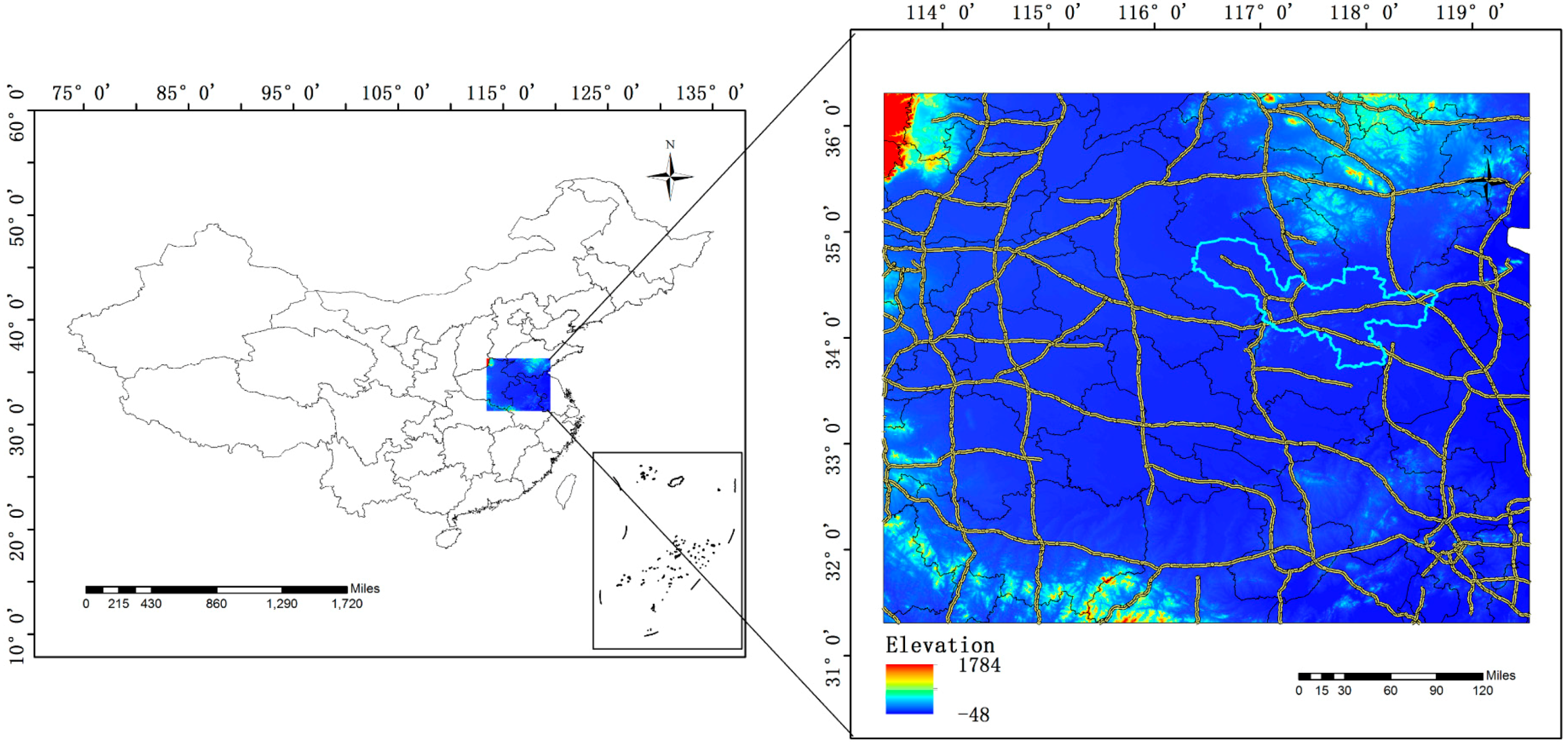
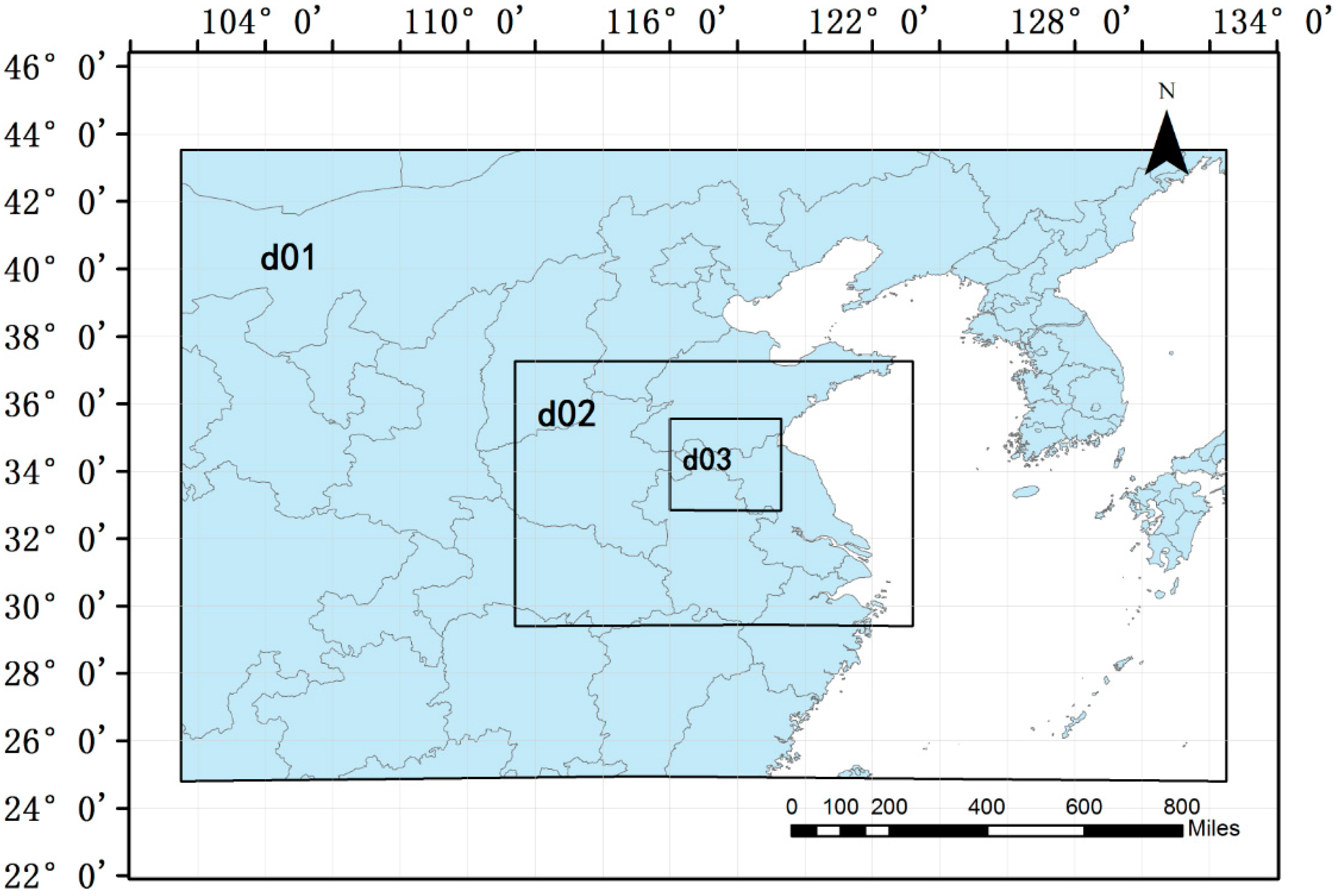
2.1. Study Area
2.2. Data Used
2.2.1. Meteorological Data
2.2.2. A Priori PM2.5 Emission Inventory
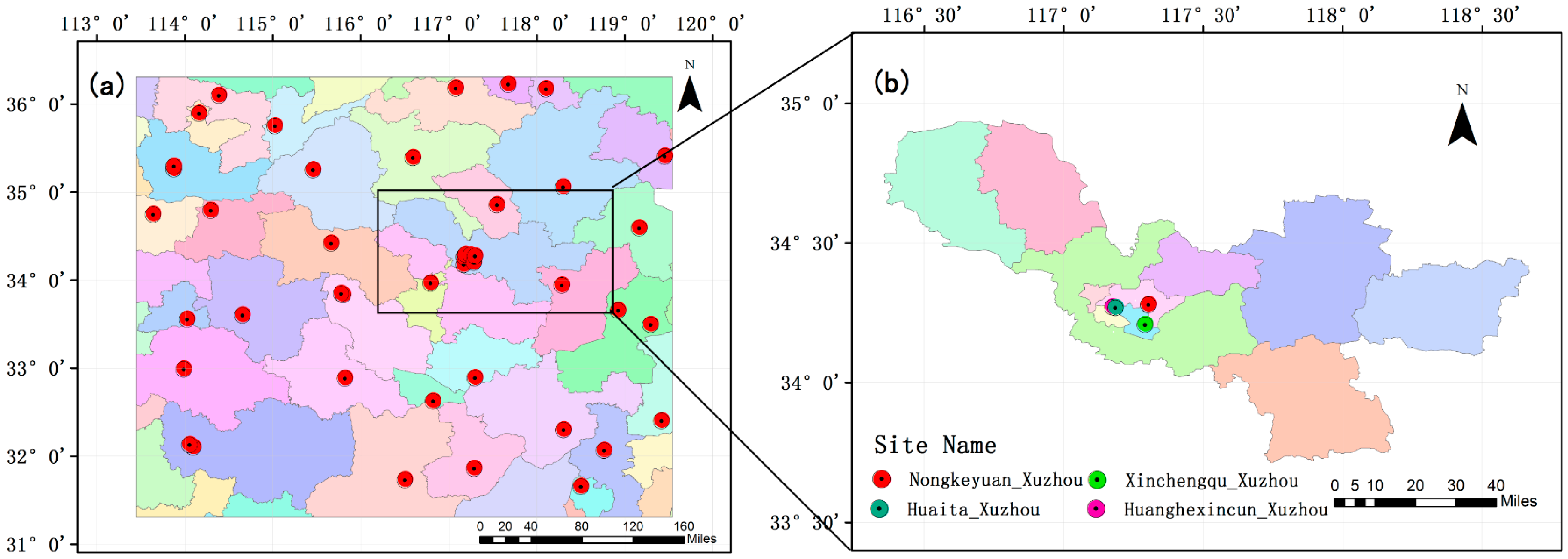
2.2.3. Observations
- Daily constant value check. If MIN(PM2.5) = MAX(PM2.5) for a 24-h period, then the entire day is eliminated.
- Outliers check. Data over 500 µg/m3 are rejected.
- Single spike. If the difference in PM2.5 concentration between the present hour () and both the previous hour () and the following hour () is greater than 50 , the data for the present hour () are rejected.
- Averaged spike. If the mean concentration over three consecutive hours () is greater than the data in the previous hour () and the following hour () by more than 80 , the data for hours () are rejected.
2.3. Model Descriptions
2.4. Inversion Method
2.4.1. Generating the Source–Receptor Relationship
2.4.2. Construction Cost Function and Calculation
2.4.3. Optimization According to the A Posteriori Inventory for Forecasting PM2.5
2.5. Verification Statistics
3. Results and Discussion
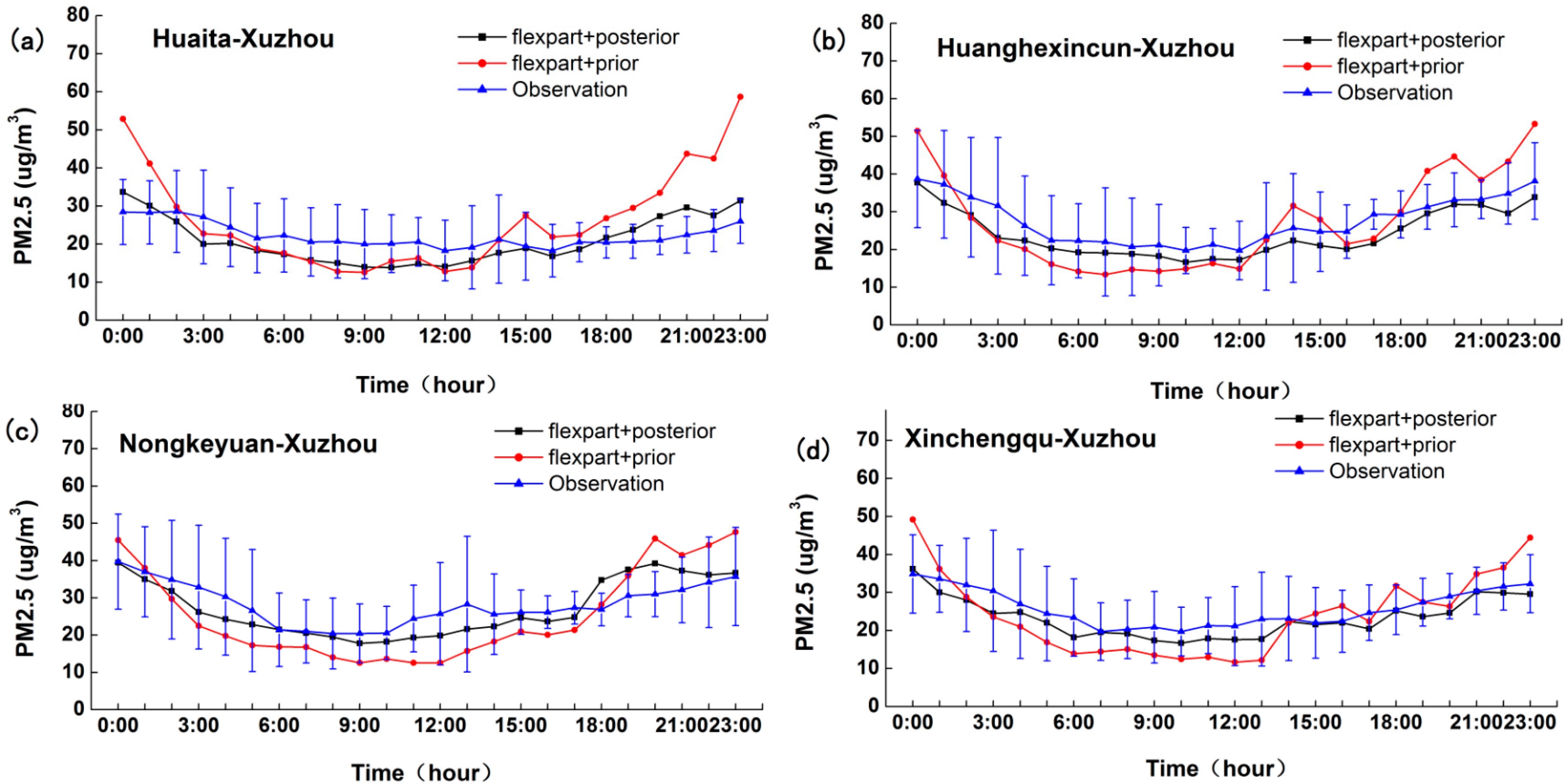
3.1. Evaluation of the Site Optimizations
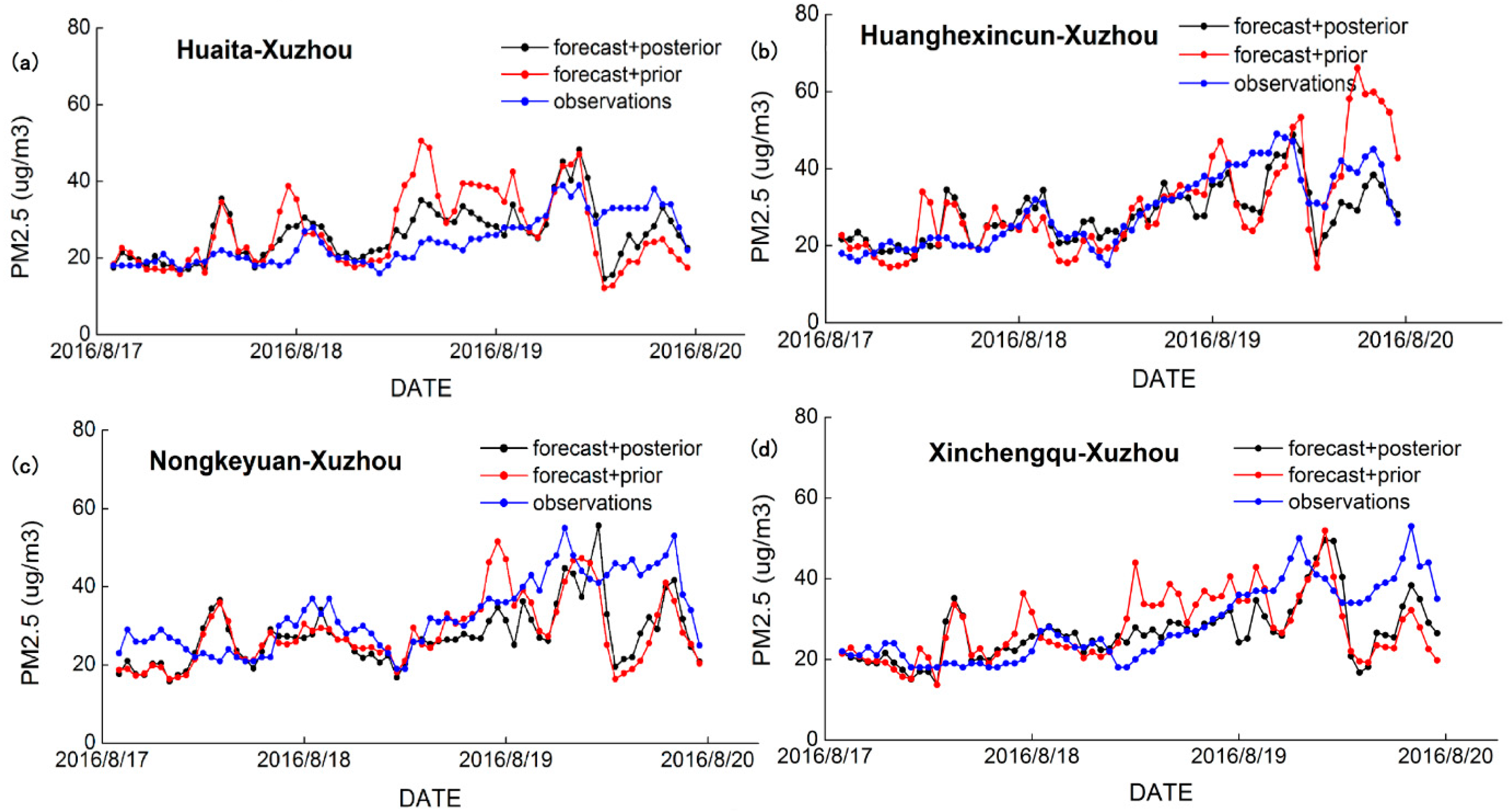
3.2. Evaluation of the Site Forecasts
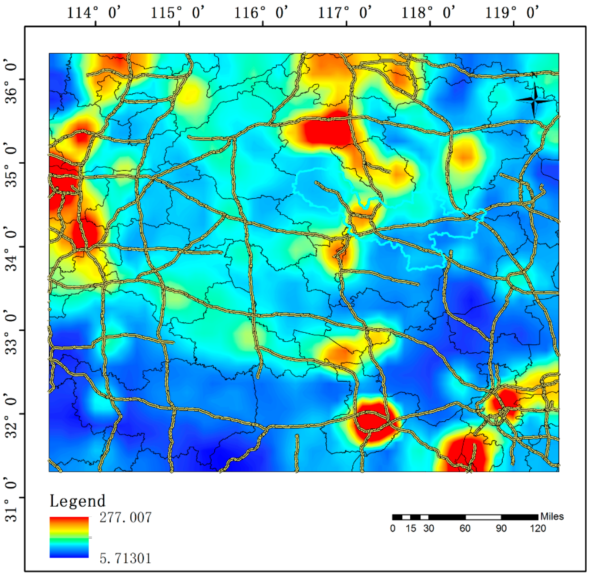
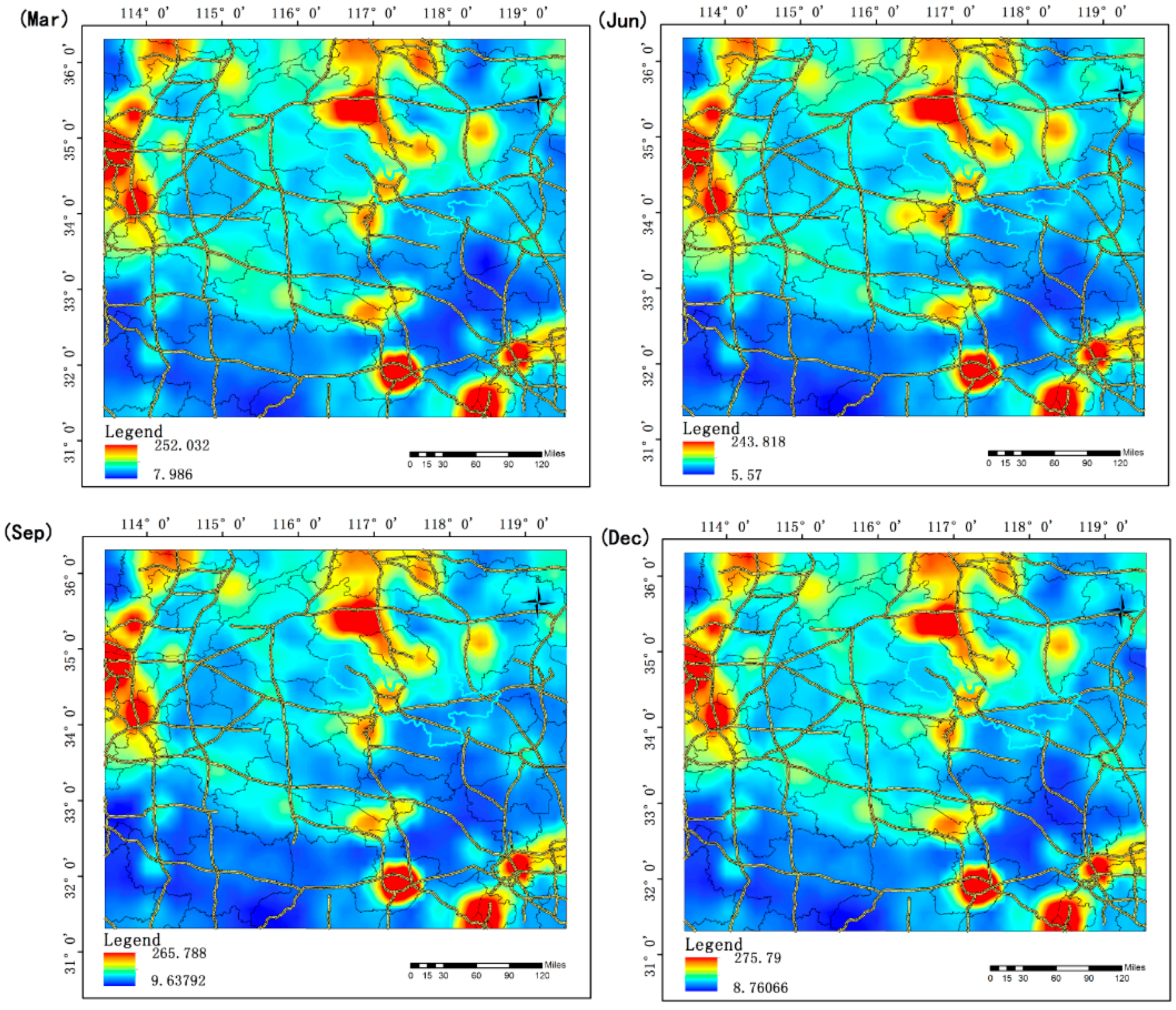
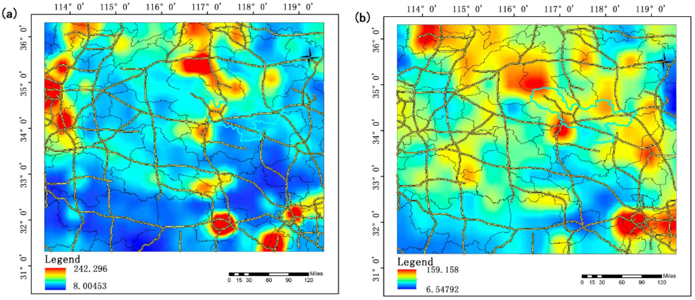
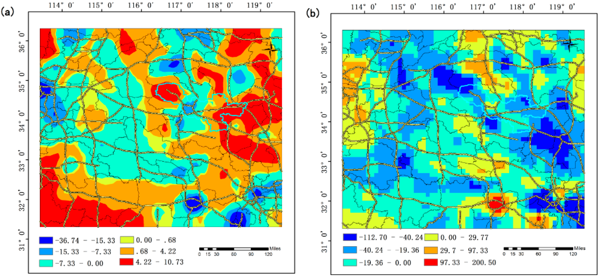
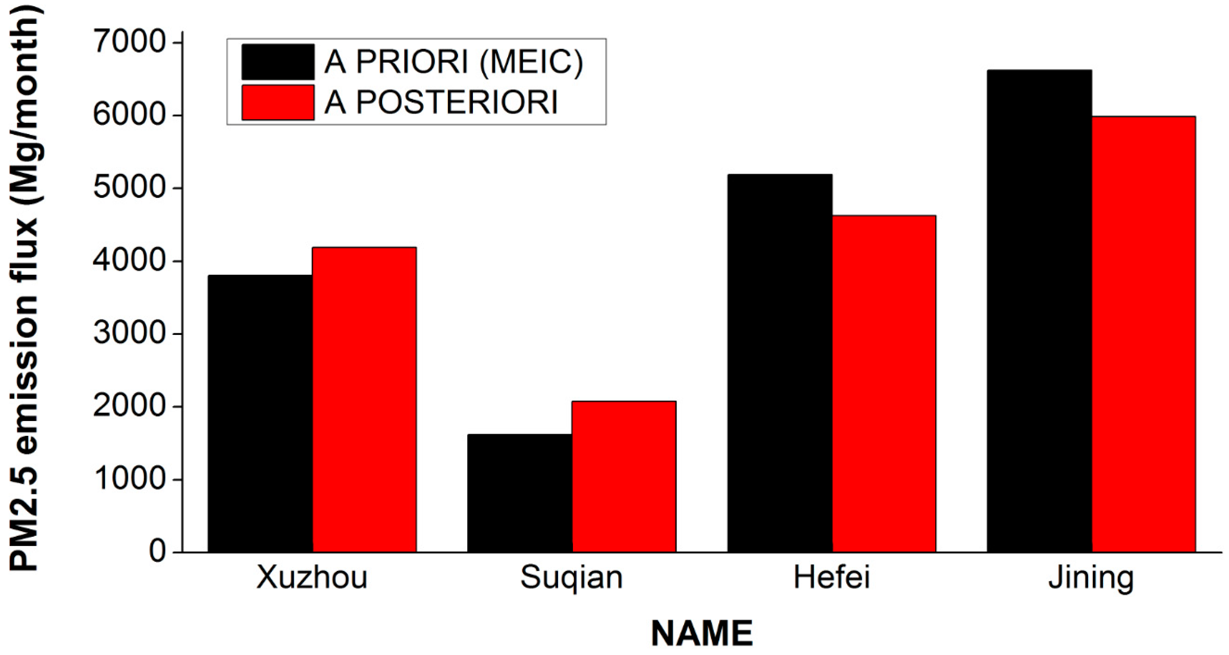
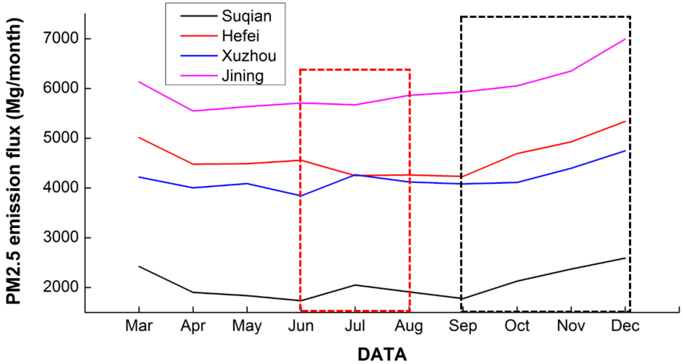
3.3. Analysis of the Emission Inventory
4. Conclusions
Author Contributions
Funding
Acknowledgments
Conflicts of Interest
References
- Zhao, X.; Shi, H.; Yu, H.; Yang, P. Inversion of Nighttime PM2.5 Mass Concentration in Beijing Based on the VIIRS Day-Night Band. Atmosphere 2016, 7, 136. [Google Scholar] [CrossRef]
- Yang, F.M.; Ma, Y.L.; He, K.B. A brief introduction to PM2.5 and related research. World Environ. 2000, 2000, 32–34. [Google Scholar]
- Zhang, Q.; Quan, J.; Tie, X.; Li, X.; Liu, Q.; Gao, Y.; Zhao, D. Effects of meteorology and secondary particle formation on visibility during heavy haze events in Beijing, China. Sci. Total Environ. 2015, 502, 578–584. [Google Scholar] [CrossRef] [PubMed]
- Yang, Y.; Liu, X.; Qu, Y.; Wang, J.; An, J.; Zhang, Y.; Zhang, F. Formation mechanism of continuous extreme haze episodes in the megacity Beijing, China, in January 2013. Atmos. Res. 2015, 155, 192–203. [Google Scholar] [CrossRef]
- Bei, N.; Xiao, B.; Meng, N.; Feng, T. Critical role of meteorological conditions in a persistent haze episode in the Guanzhong basin, China. Sci. Total Environ. 2016, 550, 273–284. [Google Scholar] [CrossRef] [PubMed]
- Cuvelier, C.; Thunis, P.; Vautard, R.; Amann, M.; Bessagnet, B.; Bedogni, M.; Berkowicz, R.; Brandt, J.; Brocheton, F.; Builtjes, P.; et al. CityDelta: A model intercomparison study to explore the impact of emission reductions in European cities in 2010. Atmos. Environ. 2007, 41, 189–207. [Google Scholar] [CrossRef]
- EPA. Guidelines for Developing an Air Quality Forecasting Program; Environmental Protection Agency Report, EPA-456/R-03-002; Environmental Protection Agency: Washington, DC, USA, 2003.
- Dong, M.; Yang, D.; Kuang, Y.; He, D.; Erdal, S.; Kenski, D. PM2.5, concentration prediction using hidden semi-Markov model-based times series data mining. Expert Syst. Appl. 2009, 36, 9046–9055. [Google Scholar] [CrossRef]
- Baklanov, A. Overview of the European project FUMAPEX. Atmos. Chem. Phys. Discuss. 2005, 5, 2005–2015. [Google Scholar] [CrossRef]
- Fay, B.; Userer, L.N. Evaluation of high-resolution forecasts with the non-hydrostaticnumerical weather prediction model Lokalmodell for urban air pollutionepisodes in Helsinki, Oslo and Valencia. Atmos. Chem. Phys. 2006, 6, 2107–2128. [Google Scholar] [CrossRef]
- Palau, J.L.; Pérezlanda, G.; Diéguez, J.J.; Monter, C.; Millán, M.M. The importance of meteorological scales to forecast air pollution scenarios on coastal complex terrain. Atmos. Chem. Phys. 2005, 5, 2771–2785. [Google Scholar] [CrossRef]
- Schroeder, A.J.; Stauffer, D.R.; Seaman, N.L.; Deng, A.; Gibbs, A.M.; Hunter, G.K.; Young, G.S. An Automated High-Resolution, Rapidly Relocatable Meteorological Nowcasting and Prediction System. Mon. Weather Rev. 2006, 134, 1237–1265. [Google Scholar] [CrossRef]
- Finardi, S.; Maria, R.D.; D’Allura, A.; Cascone, C.; Calori, G.; Lollobrigida, F. A deterministic air quality forecasting system for Torino urban area, Italy. Environ. Model. Softw. 2008, 23, 344–355. [Google Scholar] [CrossRef]
- Baklanov, A.; Mestayer, P.G.; Clappier, A.; Zilitinkevich, S.; Joffre, S.; Mahura, A.; Nielsen, N.W. Towards improving the simulation of meteorological fields in urban areas through updated/advanced surface fluxes description. Atmos. Chem. Phys. 2008, 8, 523–543. [Google Scholar] [CrossRef]
- Borrego, C.; Schatzmann, M.; Galmarini, S. Quality Assurance of Air Pollution Models. In Air Quality in Cities; Springer: Berlin/Heidelberg, Germany, 2003; pp. 155–183. [Google Scholar]
- Borrego, C.; Monteiro, A.; Ferreira, J.; Miranda, A.I.; Costa, A.M.; Carvalho, A.C.; Lopes, M. Procedures for estimation of modelling uncertainty in air quality assessment. Environ. Int. 2008, 34, 613–620. [Google Scholar] [CrossRef] [PubMed]
- Chang, J.C.; Hanna, S.R. Air quality model performance evaluation. Meteorol. Atmos. Phys. 2004, 87, 167–196. [Google Scholar] [CrossRef]
- Mckeen, S.; Wilczak, J.; Grell, G.; Djalalova, I.; Peckham, S.; Hsie, E.-Y.; Gong, W.; Bouchet, V.; Menard, S.; Moffet, R.; et al. Assessment of an ensemble of seven real-time ozone forecasts over eastern North America during the summer of 2004. J. Geophys. Res. 2005, 110, 3003–3013. [Google Scholar] [CrossRef]
- Pagowski, M.; Grell, G.A.; Devenyi, D.; Peckham, S.E.; McKeen, S.A.; Gong, W.; Monache, L.D.; McHenry, J.N.; McQueen, J.; Lee, P. Application of dynamic linear regression to improve the skill of ensemble-based deterministic ozone forecasts. Atmos. Environ. 2006, 40, 3240–3250. [Google Scholar] [CrossRef]
- Djalalova, I.; Wilczak, J.; Mckeen, S.; Grell, G.; Peckham, S.; Pagowski, M.; DelleMonache, L.; McQueen, J.; Tang, Y.; Lee, P.; et al. Ensemble and bias-correction techniques for air quality model forecasts of surface O3, and PM2.5, during the TEXAQS-II experiment of 2006. Atmos. Environ. 2010, 44, 455–467. [Google Scholar] [CrossRef]
- Sicardi, V.; Ortiz, J.; Rincón, A.; Jorba Casellas, O.; Pay Pérez, M.T.; Gassó Domingo, S.; Baldasano Recio, J.M. Ground-level ozone concentration over Spain: An application of Kalman Filter post-processing to reduce model uncertainties. Geosci. Model Dev. Discuss. 2011, 4, 343–384. [Google Scholar] [CrossRef]
- Abderrahim, H.; Chellali, M.R.; Hamou, A. Forecasting PM10, in Algiers: Efficacy of multilayer perceptron networks. Environ. Sci. Pollut. Res. Int. 2016, 23, 1634–1641. [Google Scholar] [CrossRef] [PubMed]
- Biancofiore, F.; Busilacchio, M.; Verdecchia, M.; Tomassetti, B.; Aruffo, E.; Bianco, S.; Di Tommaso, S.; Colangeli, C.; Rosatelli, G.; Di Carlo, P. Recursive neural network model for analysis and forecast of PM10 and PM2.5. Atmos. Pollut. Res. 2017, 8, 652–659. [Google Scholar] [CrossRef]
- Monache, L.D.; Nipen, T.; Deng, X.; Zhou, Y.; Stull, R. Ozone ensemble forecasts: 2. A Kalman filter predictor bias correction. J. Geophys. Res. Atmos. 2006, 111. [Google Scholar] [CrossRef]
- Kang, D.; Mathur, R.; Rao, S.T.; Yu, S. Bias adjustment techniques for improving ozone air quality forecasts. J. Geophys. Res. Atmos. 2008, 113. [Google Scholar] [CrossRef]
- Zhang, Q.; Streets, D.G.; Carmichael, G.R.; He, K.B.; Huo, H.; Kannari, A.; Klimont, Z.; Park, I.S.; Reddy, S.; Fu, J.S.; et al. Asian emissions in 2006 for the NASA INTEX-B mission. Atmos. Chem. Phys. 2009, 9, 5131–5153. [Google Scholar] [CrossRef]
- Li, Q.; Jiang, J.; Wang, S.; Rumchev, K.; Mead-Hunter, R.; Morawska, L.; Hao, J. Impacts of household coal and biomass combustion on indoor and ambient air quality in China: Current status and implication. Sci. Total Environ. 2017, 576, 347–361. [Google Scholar] [CrossRef] [PubMed]
- Brioude, J.; Arnold, D.; Stohl, A.; Cassiani, M.; Morton, D.; Seibert, P.; Angevine, W.; Evan, S.; Dingwell, A.; Fast, J.D.; et al. The Lagrangian particle dispersion model FLEXPART-WRF version 3.0. Geosci. Model Dev. Discuss. 2013, 6, 1889–1904. [Google Scholar] [CrossRef]
- Djalalova, I.; Monache, L.D.; Wilczak, J. PM2.5, analog forecast and Kalman filter post-processing for the Community Multiscale Air Quality (CMAQ) model. Atmos. Environ. 2015, 119, 431–442. [Google Scholar] [CrossRef]
- Stohl, A.; Hittenberger, M.; Wotawa, G. Validation of the Lagrangian particle dispersion model FLEXPART against largescale tracer experiment data. Atmos. Environ. 1998, 32, 4245–4264. [Google Scholar] [CrossRef]
- Fast, J.D.; Easter, R.C. A Lagrangian particle dispersion model compatible with WRF. In Proceedings of the 7th Annual WRF User’s Workshop, Boulder, CO, USA, 19–22 June 2006; pp. 19–22. [Google Scholar]
- Angevine, W.M.; Brioude, J.; McKeen, S.; Holloway, J.S.; Lerner, B.M.; Goldstein, A.H.; Guha, A.; Andrews, A.; Nowak, J.B.; Evan, S.; et al. Pollutant transport among California regions. J. Geophys. Res. Atmos. 2013, 118, 6750–6763. [Google Scholar] [CrossRef]
- Madala, S.; Satyanarayana, A.N.V.; Srinivas, C.V.; Kumar, M. Mesoscale atmospheric flowfield simulations for air quality modeling over complex terrain region of Ranchi in eastern India using WRF. Atmos. Environ. 2015, 107, 315–328. [Google Scholar] [CrossRef]
- Cécé, R.; Bernard, D.; Brioude, J.; Zahibo, N. Microscale anthropogenic pollution modelling in a small tropical island during weak trade winds: Lagrangian particle dispersion simulations using real nested LES meteorological fields. Atmos. Environ. 2016, 139, 98–112. [Google Scholar] [CrossRef]
- Srinivas, C.V.; Rakesh, P.T.; Prasad, K.H.; Venkatesan, R.; Baskaran, R.; Venkatraman, B. Assessment of atmospheric dispersion and radiological impact from the Fukushima accident in a 40 km range using a simulation approach. Air Qual. Atmos. Health 2014, 7, 209–227. [Google Scholar] [CrossRef]
- Gentner, D.R.; Ford, T.B.; Guha, A.; Boulanger, K.; Brioude, J.; Angevine, W.M.; de Gouw, J.A.; Warneke, C.; Gilman, J.B.; Ryerson, T.B.; et al. Emissions of organic carbon and methane from petroleum and dairy operations in California’s San Joaquin Valley. Atmos. Chem. Phys. 2014, 14, 4955–4978. [Google Scholar] [CrossRef]
- Marelle, L.; Raut, J.C.; Thomas, J.L.; Law, K.S.; Quennehen, B.; Ancellet, G.; Pelon, G.; Schwarzenboeck, A.; Fast, J.D. Transport of anthropogenic and biomass burning aerosols from Europe to the Arctic during spring 2008. Atmos. Chem. Phys. 2015, 15, 3831–3850. [Google Scholar] [CrossRef]
- Li, W.J.; Chen, S.R.; Xu, Y.S.; Guo, X.C.; Sun, Y.L.; Yang, X.Y.; Wang, Z.F.; Zhao, X.D.; Chen, J.M.; Wang, W.X. Mixing state and sources of submicron regional background aerosols in the northern Qinghai-Tibet Plateau and the influence of biomass burning. Atmos. Chem. Phys. 2015, 15, 13365–13376. [Google Scholar] [CrossRef]
- Pan, X.L.; Kanaya, Y.; Wang, Z.F.; Tang, X.; Takigawa, M.; Pakpong, P.; Taketani, F.; Akimoto, H. Using Bayesian optimization method and FLEXPART tracer model to evaluate CO emission in East China in springtime. Environ. Sci. Pollut. Res. Int. 2014, 21, 3873–3879. [Google Scholar] [CrossRef] [PubMed]
- Stohl, A.; Seibert, P.; Arduini, J.; Eckhardt, S.; Fraser, P.; Greally, B.R.; Maione, M.; O’Doherty, S.; Prinn, R.G.; Reimann, S.; et al. A new analytical inversion method for determining regional and global emissions of greenhouse gases: Sensitivity studies and application to halocarbons. Atmos. Chem. Phys. 2009, 69, 1026–1027. [Google Scholar] [CrossRef]
- Willmott, C.J.; Ackleson, S.G.; Davis, R.E.; Feddema, J.J.; Klink, K.M.; Legates, D.R.; O’Donnell, J.; Rowe, C.M. Statistics for the evaluation and comparison of models. J. Geophys. Res. Oceans 1985, 90, 8995–9005. [Google Scholar] [CrossRef]
- Willmott, C.J.; Matsuura, K. Advantages of the Mean Absolute Error (MAE) over the Root Mean Square Error (RMSE) in Assessing Average Model Performance. Clim. Res. 2005, 30, 79–82. [Google Scholar] [CrossRef]
- Lyu, B.; Zhang, Y.; Hu, Y. Improving PM2.5 Air Quality Model Forecasts in China Using a Bias-Correction Framework. Atmosphere 2017, 8, 147. [Google Scholar] [CrossRef]
- Borrego, C.; Monteiro, A.; Pay, M.T.; Ribeiro, I.; Miranda, A.I.; Basart, S.; Baldasano, J.M. How bias-correction can improve air quality forecasts over Portugal. Atmos. Environ. 2011, 45, 6629–6641. [Google Scholar] [CrossRef]
- Wang, H.J.; Chen, H.P. Understanding the recent trend of haze pollution in eastern China: Roles of climate change. Atmos. Chem. Phys. 2016, 16, 1–18. [Google Scholar] [CrossRef]


| A Priori | A Posteriori | |||||
|---|---|---|---|---|---|---|
| Name | R | RMSE | IOA | R | RMSE | IOA |
| Huaita | 0.638 | 11.716 | 0.445 | 0.719 | 4.575 | 0.738 |
| Huanghexincun | 0.905 | 7.371 | 0.837 | 0.957 | 4.018 | 0.901 |
| Nongkeyuan | 0.825 | 8.566 | 0.752 | 0.826 | 4.393 | 0.879 |
| Xinchengqu | 0.864 | 6.937 | 0.781 | 0.928 | 3.171 | 0.901 |
| A Priori | A Posteriori | |||||
|---|---|---|---|---|---|---|
| Site | R | RMSE | IOA | R | RMSE | IOA |
| Huaita | 0.288 | 10.188 | 0.535 | 0.593 | 6.277 | 0.762 |
| Huanghexincun | 0.687 | 9.208 | 0.804 | 0.771 | 6.157 | 0.852 |
| Nongkeyuan | 0.479 | 10.126 | 0.674 | 0.591 | 9.381 | 0.709 |
| Xinchengqu | 0.382 | 9.698 | 0.641 | 0.601 | 7.814 | 0.755 |
| Name | A Posteriori (Mg/Month) | A Priori (Mg/Month) | Difference (%) * |
|---|---|---|---|
| Xuzhou | 4188.26 | 3803.5 | 10.12 |
| Suqian | 2073.54 | 1622.04 | 27.84 |
| Hefei | 4623.47 | 5184.88 | −10.83 |
| Jining | 5987.45 | 6621.77 | −9.58 |
© 2018 by the authors. Licensee MDPI, Basel, Switzerland. This article is an open access article distributed under the terms and conditions of the Creative Commons Attribution (CC BY) license (http://creativecommons.org/licenses/by/4.0/).
Share and Cite
Guo, L.; Chen, B.; Zhang, H.; Xu, G.; Lu, L.; Lin, X.; Kong, Y.; Wang, F.; Li, Y. Improving PM2.5 Forecasting and Emission Estimation Based on the Bayesian Optimization Method and the Coupled FLEXPART-WRF Model. Atmosphere 2018, 9, 428. https://doi.org/10.3390/atmos9110428
Guo L, Chen B, Zhang H, Xu G, Lu L, Lin X, Kong Y, Wang F, Li Y. Improving PM2.5 Forecasting and Emission Estimation Based on the Bayesian Optimization Method and the Coupled FLEXPART-WRF Model. Atmosphere. 2018; 9(11):428. https://doi.org/10.3390/atmos9110428
Chicago/Turabian StyleGuo, Lifeng, Baozhang Chen, Huifang Zhang, Guang Xu, Lijiang Lu, Xiaofeng Lin, Yawen Kong, Fei Wang, and Yanpeng Li. 2018. "Improving PM2.5 Forecasting and Emission Estimation Based on the Bayesian Optimization Method and the Coupled FLEXPART-WRF Model" Atmosphere 9, no. 11: 428. https://doi.org/10.3390/atmos9110428
APA StyleGuo, L., Chen, B., Zhang, H., Xu, G., Lu, L., Lin, X., Kong, Y., Wang, F., & Li, Y. (2018). Improving PM2.5 Forecasting and Emission Estimation Based on the Bayesian Optimization Method and the Coupled FLEXPART-WRF Model. Atmosphere, 9(11), 428. https://doi.org/10.3390/atmos9110428