Source Apportionment and Data Assimilation in Urban Air Quality Modelling for NO₂: The Lyon Case Study

Abstract

Developing effective strategies for reducing the atmospheric pollutant concentrations below regulatory threshold levels requires identifying the main origins/sources of air pollution. This can be achieved by implementing so called source apportionment methods in atmospheric dispersion models. This study presents the results of a source apportionment module implemented in the SIRANE urban air-quality model. This module uses the tagged species approach and includes two methods, named SA-NO and SA-NOX, in order to evaluate the sources’ contributions to the ${\mathrm{NO}}_2$ concentrations in air. We also present results of a data assimilation method, named SALS, that uses the source apportionment estimates to improve the accuracy of the SIRANE model results. The source apportionment module and the assimilation method have been tested on a real case study (the urban agglomeration of Lyon, France, for the year 2008) focusing on the ${\mathrm{NO}}_2$ emissions and concentrations. Results of the source apportionment with the SA-NO and SA-NOX models are similar. Both models show that traffic is the main cause of ${\mathrm{NO}}_2$ air pollution in the studied area. Results of the SALS data assimilation method highlights its ability in improving the predictions of an urban atmospheric models.

1. Introduction

Obtaining information about the intensity of the pollutant sources is essential in order to determine the main causes of air pollution and to define the relevant actions for its reduction. The assessment of the intensity of the pollutant sources can rely on different criteria, namely on the estimate of the contribution of (i) different typology of sources (e.g., traffic, industry, agriculture or residential-tertiary emissions) [1,2,3,4,5], (ii) sources located in different geographical areas (e.g., emissions from different regions of Europe) [3,6,7,8], and (iii) emissions occurring at different times. The methods adopted to estimate the contribution of different sources are usually referred to as source apportionment methods, and can be classified in three main approaches.

The first is based on the analysis of the chemical composition of the pollutant. This method is essentially applied to particulate matter (PM), which is composed from a variety of chemical elements, some of which are specific to some sources [9,10,11]. For example, the black carbon reveals the emission by combustion processes [11], whereas the dehydroabietic acid is characteristic of natural sources, as coniferae [9,12].

The second is based on the so called receptor models [13,14]. These are statistical approaches, based on mass conservation principles [14], requiring as input data the concentrations measured at the monitoring stations. These models are generally classified into two different categories, known as Chemical Mass Balance (CMB) models [15,16,17,18,19] and multivariate models [17,19,20,21,22,23,24]. The receptor models are mainly used to evaluate sources of PM pollution [14,17,24,25], but can in principle also be used for other species [26,27].

The third method is based on the use of atmospheric dispersion models. These estimate the concentration field of a pollutant by solving, analytically or numerically, the advection-diffusion equation:

$${\displaystyle \frac{\partial c}{\partial t}}+\mathbf{u}\nabla c=\nabla (D_t\nabla c)+S,$$

(1)

where c is the (time) averaged pollutant concentration, $\mathbf{u}$ is the (time) averaged wind velocity, $D_t$ is the turbulent diffusivity and S represents the source terms (emissions, losses, chemical reactions). Without chemical reactions (i.e., $S=0$), Equation (1) is linear for the concentration. Therefore, sources’ contributions can be assessed by separately addressing emissions from each source. This approach is no longer valid when considering reactive pollutants because chemical reactions induce nonlinear effects. As pointed out by Koo et al. [28], this nonlinearity precludes an exact reconstruction of the sources’ contributions, which can therefore be evaluated in several different ways.

One of the simplest methods to evaluate the source effect with an atmospheric dispersion model is the so called brute force method (BFM) [3,28,29]. This is carried out in two steps. The first step consists of performing a reference simulation including all sources. The second step consists of carrying out simulations excluding some of these sources (or a typology of sources). The difference between the results of the two simulations quantifies the contribution of the sources that have been removed. Nevertheless, this method is computationally expensive because the second step has to be carried out for each source typology considered. A suitable approach to reduce the computational costs is to perform a single simulation with tagged species [1,4,5,8,28,30,31,32,33,34,35]. Tagging the emitted species allows them to be tracked and their origin to be identified: emissions of two sources ${\mathrm{S}}_{\mathrm{R}}$ and ${\mathrm{S}}_{\mathrm{B}}$, emitting the tagged species ${\mathrm{CO}}^{\mathrm{R}}$ and ${\mathrm{CO}}^{\mathrm{B}}$, provide concentration fields of ${\mathrm{CO}}^{\mathrm{R}}$ and ${\mathrm{CO}}^{\mathrm{B}}$, which corresponds to the ${\mathrm{S}}_{\mathrm{R}}$ and ${\mathrm{S}}_{\mathrm{B}}$ contributions, respectively.

Atmospheric dispersion models have been frequently used to evaluate the sources’ contributions to PM concentrations [1,5,7,8,28,35]. Studies have also been carried out to estimate the sources’ contributions to ozone [8,32,33,34], CO [36,37,38,39] and SO₂ [2,40] concentrations. All of these studies were performed with mesoscale atmospheric dispersion models. In this study, we aim instead at implementing a source apportionment module in an urban dispersion model, simulating pollutant transport at the local scale (a few tens of kilometers).

Results provided by source apportionment methods are here subsequently coupled with a data assimilation method. In the literature, any modelling approach coupling a model and field measurements in order to improve the accuracy of the prediction of a generic physical system is usually referred to as data assimilation [41,42,43,44,45]. Data assimilation methods are used since several decades in atmospheric sciences [46,47,48,49,50]. More recently, they have also been applied in air quality studies [51,52,53,54,55], mainly adopting chemical transport models [51,52,53,54,55,56,57,58,59,60,61,62,63,64,65,66,67], and more rarely with urban dispersion models [68]. Here, we present the results of a data assimilation method named Source Apportionment Least Square (SALS), developed for the SIRANE urban air quality model [69,70].

In what follows, we first present the SIRANE model and the chemical scheme implemented in it (Section 2.1 and Section 2.2). Secondly, we introduce the principles of the source apportionment modules and the data assimilation technique adopted (Section 2.3). Finally, we show the results of a real case study (Section 3), the urban Lyon agglomeration, for the year 2008.

2. Methods

2.1. The SIRANE Model

SIRANE is an operational model to simulate the atmospheric pollutants’ dispersion at the urban scale. It is based on the street network concept [69,71] and adopts parametric laws to model the main flow and dispersion processes within an urban area: advection along the street axes, turbulent transfer across the street-atmosphere interfaces, and exchanges at the street intersections. The presence of a roughness sub-layer just above the urban canopy (above roof level) is neglected and the flow is modelled as a boundary layer over a rough surface. There, the pollutants dispersion is modelled by a Gaussian plume, whose standard deviations are parametrised according to the Monin–Obukhov similarity theory. As customary for local scale dispersion models, SIRANE adopts a quasi-steady approach to deal with the unsteadiness of meteorological conditions and pollutant emissions, with an hourly time step. The input data are the urban geometry, the meteorological data, the locations and the modulations of the emissions (represented as point, line, and surface sources) and the hourly evolution of the background concentration, i.e., the concentration due to sources placed outside the domain. More details on the SIRANE model can be found in Soulhac et al. [69] and Soulhac et al. [72].

2.2. Modelling Chemical Reactions

The only chemical reactions taken into account in the SIRANE model concern the ${\mathrm{NO}}_2-\mathrm{NO}-{\mathrm{O}}_3$ cycle. In steady state conditions, i.e., at the photo-stationary equilibrium, this is usually represented by the following set of reactions [73]:

$$\{\begin{array}{}\mathrm{(2a)}& {\mathrm{NO}}_2+\mathrm{h}\nu \stackrel{k_1}{\to }\mathrm{NO}+{\mathrm{O}}^{•},\hfill \mathrm{(2b)}& {\mathrm{O}}^{•}+{\mathrm{O}}^2+\mathrm{M}\stackrel{k_2}{\to }{\mathrm{O}}^3+\mathrm{M},\hfill \mathrm{(2c)}& \mathrm{NO}+{\mathrm{O}}^3\stackrel{k_3}{\to }{\mathrm{NO}}_2+{\mathrm{O}}^2,\hfill \end{array}$$

where $k_1$, $k_2$, and $k_3$ are the kinetic constants of reaction and M is a third body species, e.g., O₂ and N₂. Note that the cycle (2) is in reality perturbed by other reactions, as [74]:

$$\{\begin{array}{}\mathrm{(3a)}& {\mathrm{RO}}_2+\mathrm{NO}\to {\mathrm{NO}}_2+\mathrm{RO},\hfill \mathrm{(3a)}& {\mathrm{HO}}_2+\mathrm{NO}\to {\mathrm{NO}}_2+\mathrm{OH},\hfill \end{array}$$

where the RO₂ radical is due to VOC oxidation, occurring over different times scale (larger than those of Equation (2)), depending on VOC chemical lifetime (typically a few hours). Nitroxen oxide concentrations can also be affected by losses due to reactions involving the hydroxyl radical OH, and leading to the production of nitric acid:

$$\begin{array}{c}\hfill \mathrm{OH}+{\mathrm{NO}}_2+\mathrm{M}\to {\mathrm{HNO}}_3+\mathrm{M}.\end{array}$$

(4)

For typical OH concentration in the urban atmosphere (6 × 10⁶ molec cm⁻³), the NO_x chemical lifetime is approximately 4 h, i.e., similar to the time scales of advection across a large urban agglomeration.

As is customary in dispersion models at the local scale [75], reactions (3) and (4) are neglected, and the modelling of chemical transformation of nitrogen oxide relies on Equation (2) only. Since the radical O^• is very reactive, the characteristic time of ozone production (2b) is much smaller than that of the two other reactions, so that the photo-stationary equilibrium (2) can be further simplified as:

$$\left[\begin{array}{c}\hfill {\mathrm{NO}}_2\end{array}\right]={\displaystyle \frac{k_3}{k_1}}\left[\begin{array}{c}\hfill {\mathrm{O}}_3\end{array}\right]\left[\begin{array}{c}\hfill \mathrm{NO}\end{array}\right],$$

(5)

where $\left[\begin{array}{c}\hfill \mathrm{NO}\end{array}\right]$, $\left[\begin{array}{c}\hfill {\mathrm{NO}}_2\end{array}\right]$ and $\left[\begin{array}{c}\hfill {\mathrm{O}}_3\end{array}\right]$ represent the NO, N₂, and O₃ molar concentrations, respectively. To estimate the NO, N₂, and O₃ concentrations, it is then necessary to determine $k_1$ and $k_3$ (for each hourly time step), which can be conveniently modelled as [73,76]:

$$\left\{\begin{array}{c}{k}_1={\displaystyle \frac{1}{60}}\left(0.5699-{\left[9.056e^{-3}(90-\chi )\right]}^{2.546}\right)\left(1-0.75{\left[{\displaystyle \frac{\mathrm{Cld}}{8}}\right]}^{3.4}\right)\left[{\mathrm{s}}^{-1}\right],\hfill \\ k_3=1.325e^{6}exp\left(-{\displaystyle \frac{1430}{T}}\right)\left[{\mathrm{m}}^3{\mathrm{mole}}^{-1}{\mathrm{s}}^{-1}\right],\hfill \end{array}\right.$$

(6)

where $\chi$ is the solar elevation, Cld is the cloud cover, and T is the temperature.

As already mentioned, Equation (2) represents an over-simplification of the chemical processes occurring in the urban atmosphere. Nevertheless, validation studies [70,72] show good agreement between SIRANE results, obtained adopting this simplified chemical scheme, and on-site measurements.

2.3. Source Apportionment Module

When activating the source apportionment module in the SIRANE model, the sources emit both classical species (e.g., NO and tagged species (e.g., ${\mathrm{NO}}^g$ for the source g). In simulating their dispersion in the atmosphere, as a first step, these are both treated as inert species. The role of chemical reactions is then taken into account in a second step of the simulation. The concentration of the species s is denoted as $c_s^d$ at the end of the dispersion phase and as $c_s$ after the chemical reactions phase. Similarly, the concentration of the species s tagged from the source g is denoted $c_{s,g}^d$, after the dispersion phase, and $c_{s,g}$, at the end of the chemical reactions.

2.3.1. Inert Pollutant Species

Tagged species emitted by each source are treated as different species (e.g., NO^traffic and NO^industrial). In this way, we avoid performing G separate simulations to evaluate the contribution of G sources (or group of sources) for N species, performing instead a single simulation taking into account $G\times N$ species, reducing the computational costs.

2.3.2. Reactive Pollutant Species

The assessment of the sources’ contributions for the reactive species is carried out in two steps. The first step consists of determining the sources’ contributions after their emission and their atmospheric dispersion, as happens for inert species. The second step consists of evaluating the sources’ contributions once the chemical reactions took place. The source module apportionment integrates two models, named SA-NO and SA-NOX. In both, it is assumed that molecules of a same species have the same probability of reacting, independently of their origin [1]. Both take into account the chemical reactions included in Equation (2c) only, but in a different way. In the SA-NO model, we assume that the photo-stationary equilibrium has not been reached, so that the chemical reactions (2c) occurs from the left to the right only. In the SA-NOX model, we assume instead that the photo-stationary equilibrium has already been reached, and that (2c) can be expressed in the form of a dynamical equilibrium:

$$\mathrm{NO}+{\mathrm{O}}_3\rightleftharpoons {\mathrm{NO}}_2+{\mathrm{O}}_2.$$

(7)

Model SA-NO

The mass concentration of the specie s (NO, NO₂ or O₃) after the chemical reactions can be expressed as:

$$c_s=c_s^d+\delta c_s,$$

(8)

where $\delta c_s$ is the variation induced by the chemical reactions. The contribution of a source g for the species s after the chemical reactions is then:

$$c_{s,g}=c_{s,g}^d+\delta c_{s,g},$$

(9)

where $\delta c_{s,g}$ is the contribution of the source g to the concentration variation of the species s due to chemical reactions. The objective of the SA-NO method is to determine $\delta c_{s,g}$. Since ${\mathrm{NO}}_x$ emissions are predominantly NO emissions [77], we assume that the ratio $\left[c_{\mathrm{NO}}^d\right]/\left[c_{{\mathrm{NO}}_2}^d\right]$ after the dispersion modelling phase (before modelling chemical reactions) is higher than the ratio $\left[c_{\mathrm{NO}}\right]/\left[c_{{\mathrm{NO}}_2}\right]$ at the photo-stationary equilibrium (after the chemical reactions), whose achievement requires NO molecules to be consumed and NO₂ molecules to be produced. Since the probability that a NO molecule is involved in a chemical reaction is independent of its origin, the relative sources’ contributions to the NO concentration variation is equal to their relative contribution to the NO concentration at the end of the dispersion phase:

$$\frac{c_{\mathrm{NO},g}^d}{c_{\mathrm{NO}}^d}=\frac{\delta c_{\mathrm{NO},g}}{\delta c_{\mathrm{NO}}}.$$

(10)

The variation of O₃ and NO₂ molar concentration induced by (2c) is directly related to the variation of NO moles. The relative sources’ contributions to O₃ and NO₂ concentration variation is then equal to their relative contribution to NO concentration at the end of the dispersion phase:

$$\frac{c_{\mathrm{NO},g}^d}{c_{\mathrm{NO}}^d}=\frac{\delta c_{{\mathrm{NO}}_2,g}}{\delta c_{{\mathrm{NO}}_2}}=\frac{\delta c_{{\mathrm{O}}_3,g}}{\delta c_{{\mathrm{O}}_3}}=\frac{\delta c_{s,g}}{\delta c_s}.$$

(11)

Thus, the SA-NO method evaluates the contribution of each source g as:

$$c_{s,g}=c_{s,g}^d+\delta c_s{\displaystyle \frac{c_{\mathrm{NO},g}^d}{c_{\mathrm{NO}}^d}}.$$

(12)

Note that, with the SA-NO method, the sources’ contributions may be negative, namely when the concentration computed after chemical reaction ($c_s$) is lower than that before ($c_s^d$). In addition, (12) indicates that a source contributes to NO concentrations only if it emits NO. This constitutes an evident shortcoming of the SA-NO method since, according to the NO₂-NO-O₃ cycle (2), NO concentrations can be enhanced also by contributing to NO₂ and O₃ concentration.

Model SA-NOX

Based on the fact that the relative sources’ contributions to NO_x concentration (NO + NO₂) are the same before and after the chemical reactions, we can write:

$${\displaystyle \frac{\left[c_{\mathrm{NO},g}^d\right]+\left[c_{{\mathrm{NO}}_2,g}^d\right]}{\left[c_{\mathrm{NO}}^d\right]+\left[c_{{\mathrm{NO}}_2}^d\right]}}={\displaystyle \frac{\left[c_{\mathrm{NO},g}\right]+\left[c_{{\mathrm{NO}}_2,g}\right]}{\left[c_{\mathrm{NO}}\right]+\left[c_{{\mathrm{NO}}_2}\right]}}.$$

(13)

By further assuming that the relative sources’ contributions to NO and NO₂ concentrations are the same as their relative contribution to NO_x concentration, we have that:

$${\displaystyle \frac{c_{\mathrm{NO},g}}{c_{\mathrm{NO}}}}={\displaystyle \frac{c_{{\mathrm{NO}}_2,g}}{c_{{\mathrm{NO}}_2}}}={\displaystyle \frac{\left[c_{\mathrm{NO},g}\right]+\left[c_{{\mathrm{NO}}_2,g}\right]}{\left[c_{\mathrm{NO}}\right]+\left[c_{{\mathrm{NO}}_2}\right]}}.$$

(14)

The SA-NOX method then evaluates the sources’ contributions to NO and NO₂ concentration by estimating their contribution to the nitrogen atoms of these molecules:

$$c_{s,g}=c_s{\displaystyle \frac{\left[c_{\mathrm{NO},g}^d\right]+\left[c_{{\mathrm{NO}}_2,g}^d\right]}{\left[c_{\mathrm{NO}}^d\right]+\left[c_{{\mathrm{NO}}_2}^d\right]}}.$$

(15)

Differently from the SA-NO model, (15) guarantees the contribution of all sources to be positive. Note also that, differently from the SA-NO method, a source can contribute to NO concentrations also by emitting NO₂ (or eventually O₃).

2.4. Data Assimilation Using Source Apportionment Results

The source apportionment results provide useful information that can be used to improve the performances of the dispersion model by means of the data assimilation techniques. Here, we present a data assimilation method called a Source Apportionment Least Square method (SALS). This method consists of modulating, in an optimal way, the sources’ contributions estimated with a source apportionment method.

We represent the simulated ground level concentration field $c(x,y)$, over n grid points and at a given time t, as a vector ${\mathbf{c}}_{\mathit{t}}$ of size n. This vector, called background, is then expressed as the sum of different vectors ${\mathbf{c}}_{\mathit{g},\mathit{t}}$, each of them representing the modelled contribution to ${\mathbf{c}}_{\mathit{t}}$ due to the different g sources:

$${\mathbf{c}}_{\mathit{t}}=\sum _g^G{\mathbf{c}}_{\mathit{g},\mathit{t}},$$

(16)

where G is the number of the different sources (or groups of sources). The aim of the SALS method is to obtain estimates of the ${\mathbf{c}}_{\mathit{t}}$ as close as possible to their corresponding measured value. More precisely, the objective is estimating a vector, named analysis and referred to as ${\widehat{\mathbf{c}}}_{\mathit{t}}$, defined as a linear combination of the sources’ contributions:

$${\widehat{\mathbf{c}}}_{\mathit{t}}=\sum _g^G{\alpha }_{g,t}{\mathbf{c}}_{\mathit{g},\mathit{t}},$$

(17)

where ${\alpha }_{g,t}$ is the (time dependent) modulation coefficient, related to the sources g at the time t. The analysis ${\widehat{\mathbf{c}}}_{\mathit{t}}$ is evaluated by computing ${\alpha }_{g,t}$ coefficients minimizing the cost function J (representing the quadratic error):

$$J({\alpha }_{1,t},{\alpha }_{2,t},\dots ,{\alpha }_{G,t})={\displaystyle \frac{1}{m_t}}{\left({\mathbf{y}}_{\mathit{t}}-\sum _g^G{\alpha }_{g,t}{\mathbf{H}}_{\mathit{t}}{\mathbf{c}}_{\mathit{g},\mathit{t}}\right)}^{\mathrm{T}}\left({\mathbf{y}}_{\mathit{t}}-\sum _g^G{\alpha }_{g,t}{\mathbf{H}}_{\mathit{t}}{\mathbf{c}}_{\mathit{g},\mathit{t}}\right),$$

(18)

where ${\mathbf{y}}_{\mathit{t}}$ is a vector containing the $m_t$ measurement (at the time step t). The matrix ${\mathbf{H}}_{\mathit{t}}$, called observation operator, is a matrix of size $m_t\times n$ filled of 0 and 1. When applied to the background vector ${\mathbf{c}}_{\mathit{g},\mathit{t}}$, it provides a vector of size $m_t$ containing the modelled concentrations at the same location of the measured ones (and at a given time t). The coefficients ${\alpha }_{g,t}$, considered as uniform over the whole domain (for each time step and each source contribution), are therefore determined by solving the following system:

$$\left(\begin{array}{ccc}{\left({\mathbf{H}}_{\mathit{t}}{\mathbf{c}}_{1,\mathit{t}}\right)}^{\mathrm{T}}\left({\mathbf{H}}_{\mathit{t}}{\mathbf{c}}_{1,\mathit{t}}\right)& \dots & {\left({\mathbf{H}}_{\mathit{t}}{\mathbf{c}}_{1,\mathit{t}}\right)}^{\mathrm{T}}\left({\mathbf{H}}_{\mathit{t}}{\mathbf{c}}_{\mathit{G},\mathit{t}}\right)\\ ⋮& \ddots & ⋮\\ {\left({\mathbf{H}}_{\mathit{t}}{\mathbf{c}}_{\mathit{G},\mathit{t}}\right)}^{\mathrm{T}}\left({\mathbf{H}}_{\mathit{t}}{\mathbf{c}}_{1,\mathit{t}}\right)& \dots & {\left({\mathbf{H}}_{\mathit{t}}{\mathbf{c}}_{\mathit{G},\mathit{t}}\right)}^{\mathrm{T}}\left({\mathbf{H}}_{\mathit{t}}{\mathbf{c}}_{\mathit{G},\mathit{t}}\right)\end{array}\right)\left(\begin{array}{c}{\alpha }_{1,t}\\ ⋮\\ {\alpha }_{G,t}\end{array}\right)=\left(\begin{array}{c}{\left({\mathbf{y}}_t\right)}^{\mathrm{T}}\left({\mathbf{H}}_{\mathit{t}}{\mathbf{c}}_{1,\mathit{t}}\right)\\ ⋮\\ {\left({\mathbf{y}}_t\right)}^{\mathrm{T}}\left({\mathbf{H}}_{\mathit{t}}{\mathbf{c}}_{\mathit{G},\mathit{t}}\right)\end{array}\right).$$

(19)

The resolution of the system (19), that can be typically obtained by solving a least square problem, is here carried out with the method of Lawson and Hanson [78], which guarantees the coefficients ${\alpha }_{g,t}$ to be positive. The SALS method can be applied only when $m_t\ge G$, i.e., when the measurements number $m_t$ is higher than the number of sources G. The choice of the sources (number and/or type) is a key element in the SALS method. Sources can be grouped based on their corresponding activity sectors (transport, industry, residential-tertiary, agriculture) or on their geographical localisation. Note that, for inert species (or low-reactive species), the application of the SALS method, i.e., the modulation of the sources’ contributions, can be interpreted as a method to correct the intensity of the emissions.

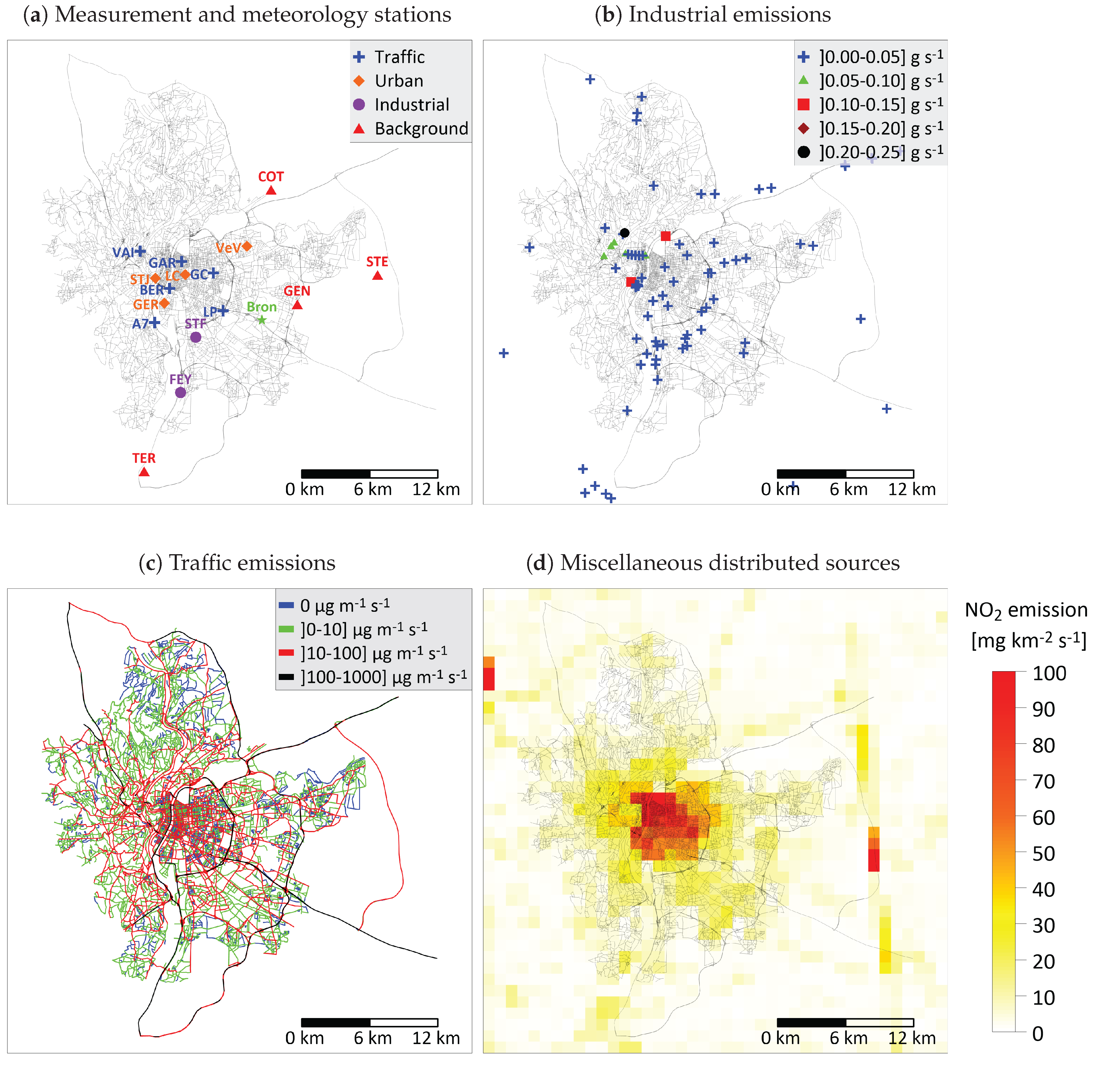
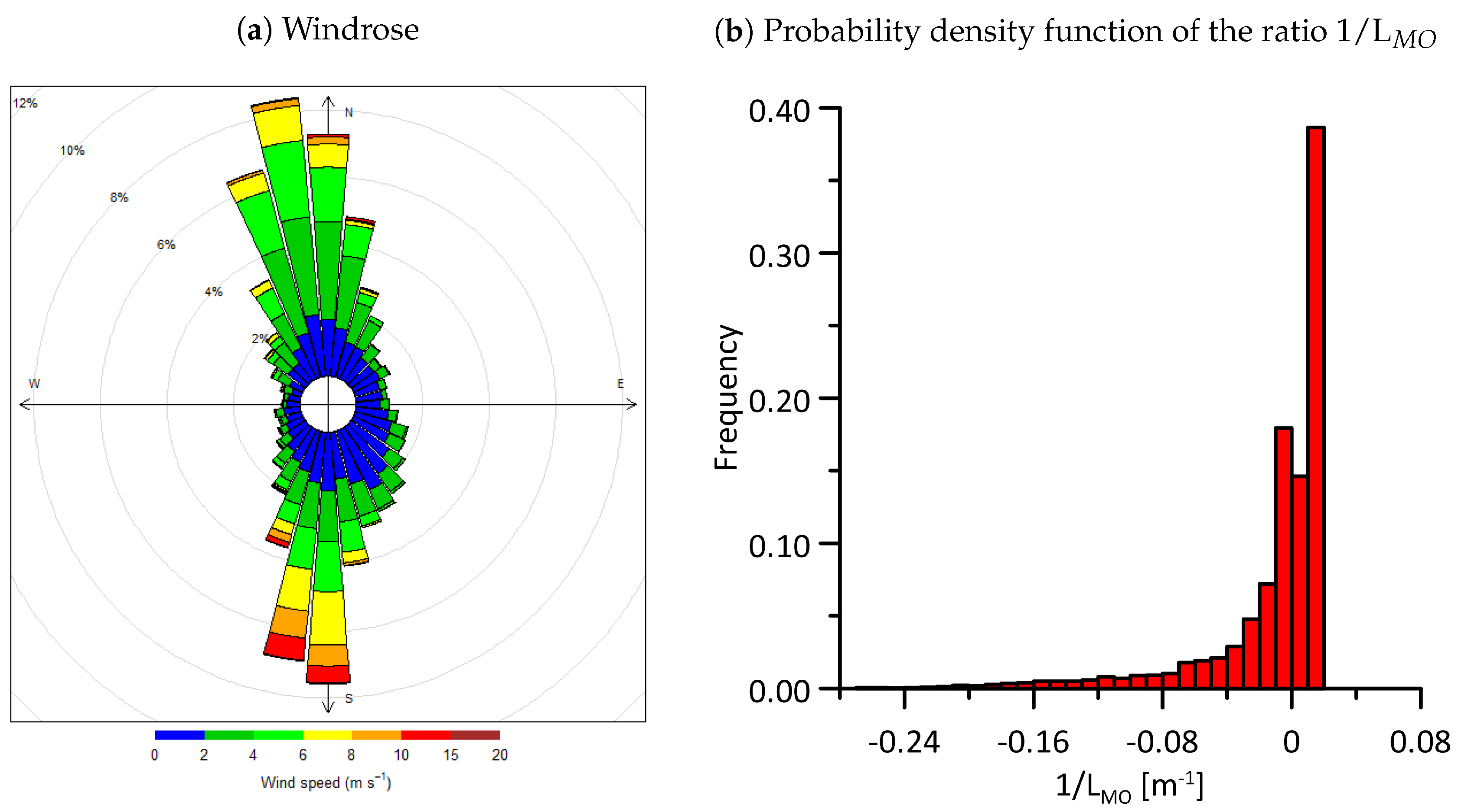
3. Case Study—The Lyon Urban Agglomeration

We present an application of the source apportionment module (with the SA-NO and the SA-NOX models) to evaluate the source contribution to NO₂ concentration on the Lyon urban agglomeration (approximately 1.4 million people) , for the year 2008. The case study is the same as that used for an extensive analysis of the performances of the SIRANE model, recently presented by Soulhac et al. [72].

We consider the contributions by three typologies of pollutant sources, namely (i) traffic, (ii) industrial sources, and (iii) miscellaneous distributed sources (all other sources not included in the two previous categories, mainly domestic heating), as well as that due to the background concentration (Figure 1a), i.e., related to all sources that are placed outside the studied domain.

Simulations were run over a 36 km × 40 km domain, with a spatial resolution of 10 m. The traffic and industrial emissions are represented by 21833 line sources and 83 point sources, respectively. Miscellaneous distributed sources are represented by surface emissions with a 1 km × 1 km resolution. The annual averaged emissions are represented in Figure 1. Most of the point sources do not exceed $0.05$ g s⁻¹ (Figure 1b), and the largest emissions are related to chimneys of road tunnels. The traffic emissions are higher in the city centre and along the main roads (Figure 1c). Miscellaneous distributed emissions are higher on the centre of the agglomeration (Figure 1d).

In the simulation, the background concentrations of the different species are assumed to be equal to those measured at the Saint-Exupéry (STE) station, located at about 20 km from the Lyon city center (see Figure 1a).

The meteorological wind field was reconstructed with an hourly time-step and according to the Monin-Obuhkov similarity theory, from data registered at the Météo-France station in Bron (Figure 1a). The dominant wind direction is North–South, with wind speeds that rarely exceed 6 m s⁻¹ (Figure 2a). The stability conditions computed by the meteorological pre-processor are presented in (Figure 2b), where we plot the inverse of the Monin–Obukhov length (L${}_{\mathrm{MO}}$). The distribution of the ratio 1/L${}_{\mathrm{MO}}$ suggests an equal repartition between stable (L${}_{\mathrm{MO}}$ > 0) and unstable (L${}_{\mathrm{MO}}$ < 0) atmospheric conditions. The high frequency of the condition 1/L${}_{\mathrm{MO}}$ in the range 0.01–0.02 is due to the fact that we have imposed a minimum value for L${}_{\mathrm{MO}}$. The purpose of this is to avoid stability conditions (here estimated by means of cloud cover measurements) that rarely occur over an urban area, due to the heat anthropogenic fluxes and the wind shear induced by the presence of the urban canopy. Further details on the input data and the model set-up can be found in Soulhac et al. [72].

Time-series of NO₂ concentration used to evaluate the SALS data assimilation method were collected in different measurement sites over the whole year 2008 by Atmo Auvergne Rhône-Alpes (AURA), the local authority for air quality. These include hourly measurements provided by 16 permanent measurement stations, which have been classified by Atmo AURA into four different categories: suburban stations (Côtière de l’Ain, Genas, Saint-Exupéry and Ternay) placed on high-intensity traffic roads (Berthelot, Grandclément, Lyon périphérique, Mulatière and Vaise), stations close to industrial sites (Feyzin and Saint-Fons) and stations within the urban agglomeration and away from high-intensity traffic roads (Gerland, Lyon centre, Saint-Just and Vaulx-en-Velin). For all these stations, missing hourly data do not exceed 3% over the whole year 2008.

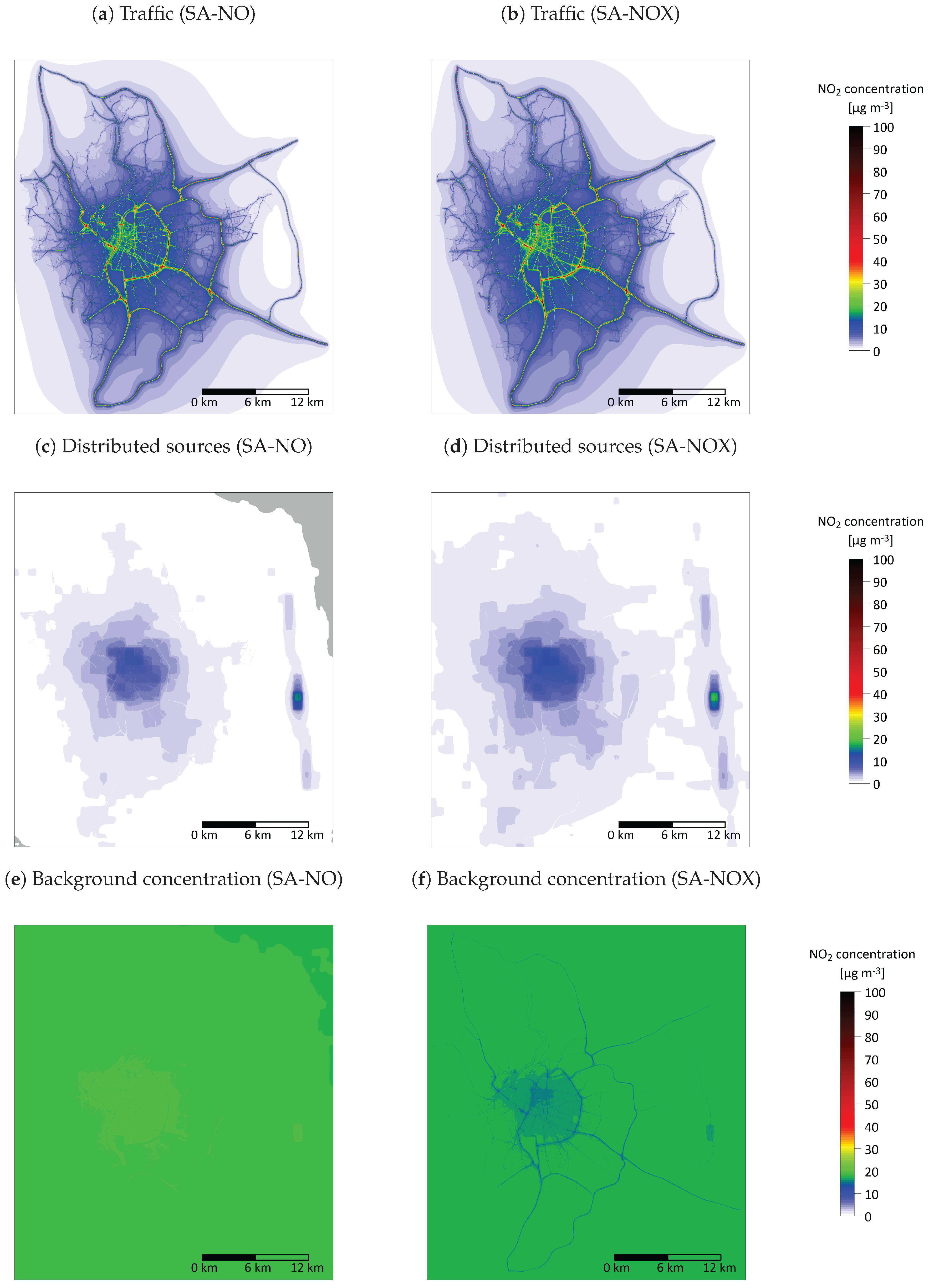
3.1. Source Apportionment Results

3.1.1. Comparison of the Results Obtained with the SA-NO and SA-NOX Models

The contribution of traffic, miscellaneous distributed sources, industry and background concentration to NO₂ annual mean concentration estimated by the SA-NO and SA-NOX models are shown in Figure 3 and Figure 4. A relevant difference between the two models is related to the negative contributions of the miscellaneous distributed sources estimated by the SA-NO model (Figure 3). According to the SA-NO model formulation (12), these negative contributions indicate that NO₂ concentrations are higher after the first step of the simulation (i.e., before the occurrence of chemical reactions) and that the miscellaneous distributed sources contribute to a consumption of NO₂ molecules larger than its initial (before chemical reactions) contribution. Similar considerations hold for industrial sources (not shown in Figure 3). The contribution of traffic and the miscellaneous distributed sources’ contributions are slightly higher when estimated with with the SA-NOX model (on average these are larger of approximately $0.59$ $\mathsf{\mu }$g m⁻³ and $0.49$ $\mathsf{\mu }$g m⁻³ for the miscellaneous distributed sources and the traffic, respectively). At the measurement stations’ locations, the mean difference is slightly larger than over the whole agglomeration and is equal to $1.90$ $\mathsf{\mu }$g m⁻³ for the miscellaneous distributed sources, and to $2.01$ $\mathsf{\mu }$g m⁻³ for traffic. On the other hand, the contribution of the background concentration is slightly higher when estimated with the SA-NO model. On average, these exceed those estimated by means of the SA-NOX model by $1.07$ $\mathsf{\mu }$g m⁻³, when considering the whole agglomeration, and by $3.96$ $\mathsf{\mu }$g m⁻³, when considering the measurement stations only.

In summary, we observe a clear tendency of the SA-NO model in overestimating background contribution (with respect to the SA-NOX model), and therefore in underestimating the relative contribution of all other sources. This is due to the fact that, for the background concentration, the relative NO₂ contribution (to the total NO₂ concentration) is inevitably higher than the relative NO_x contribution (to the total NO_x concentration). This enhanced NO₂ contribution of the background concentration is emphasised in the formulation of the SA-NO model, notably by the first term, the r.h.s of Equation (12).

Despite these slight differences, results obtained with the SA-NO and SA-NOX models are very similar. In what follows, we will however exploit only the results of the SA-NOX model, since it guarantees the contribution of all pollutant sources to be positive.

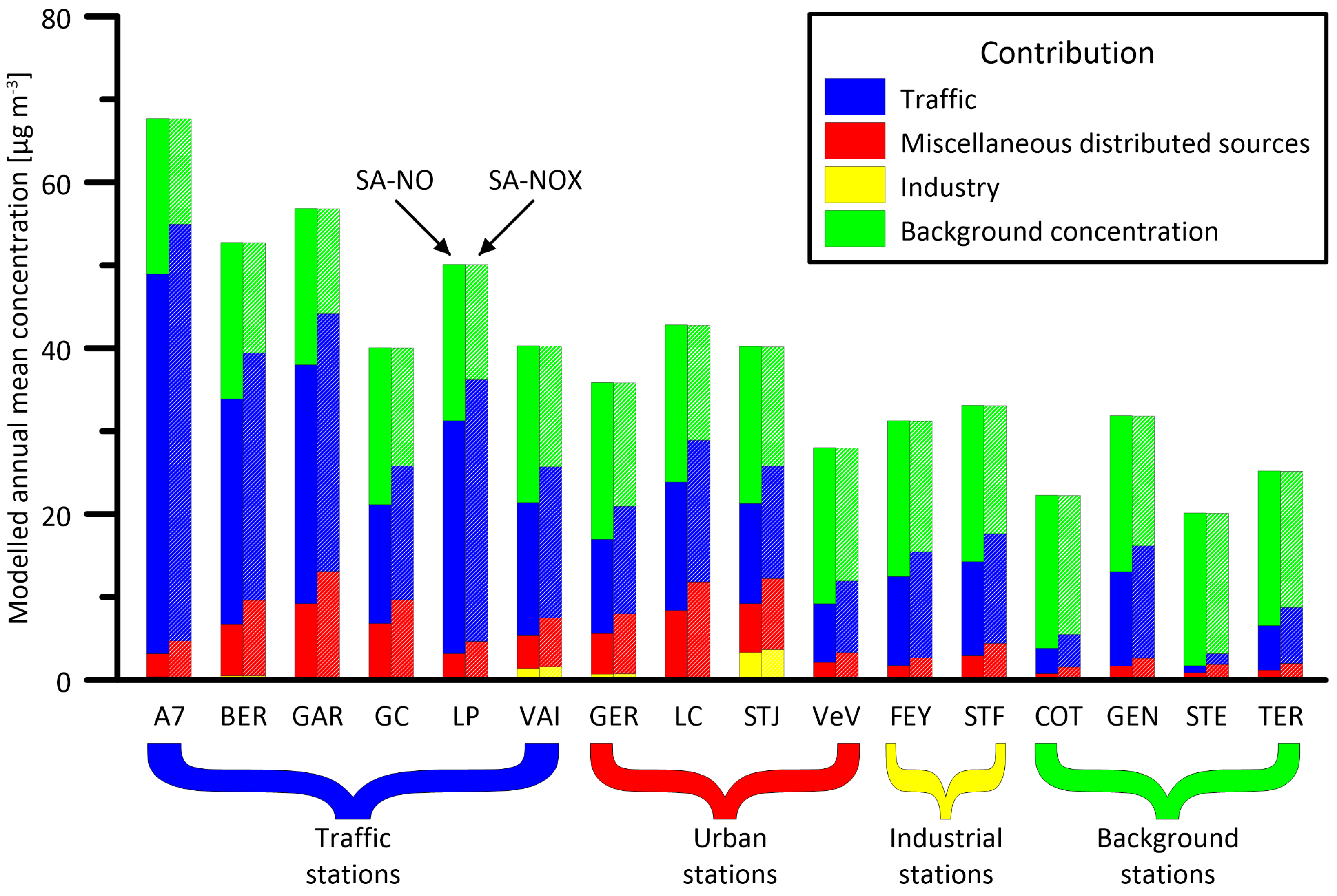
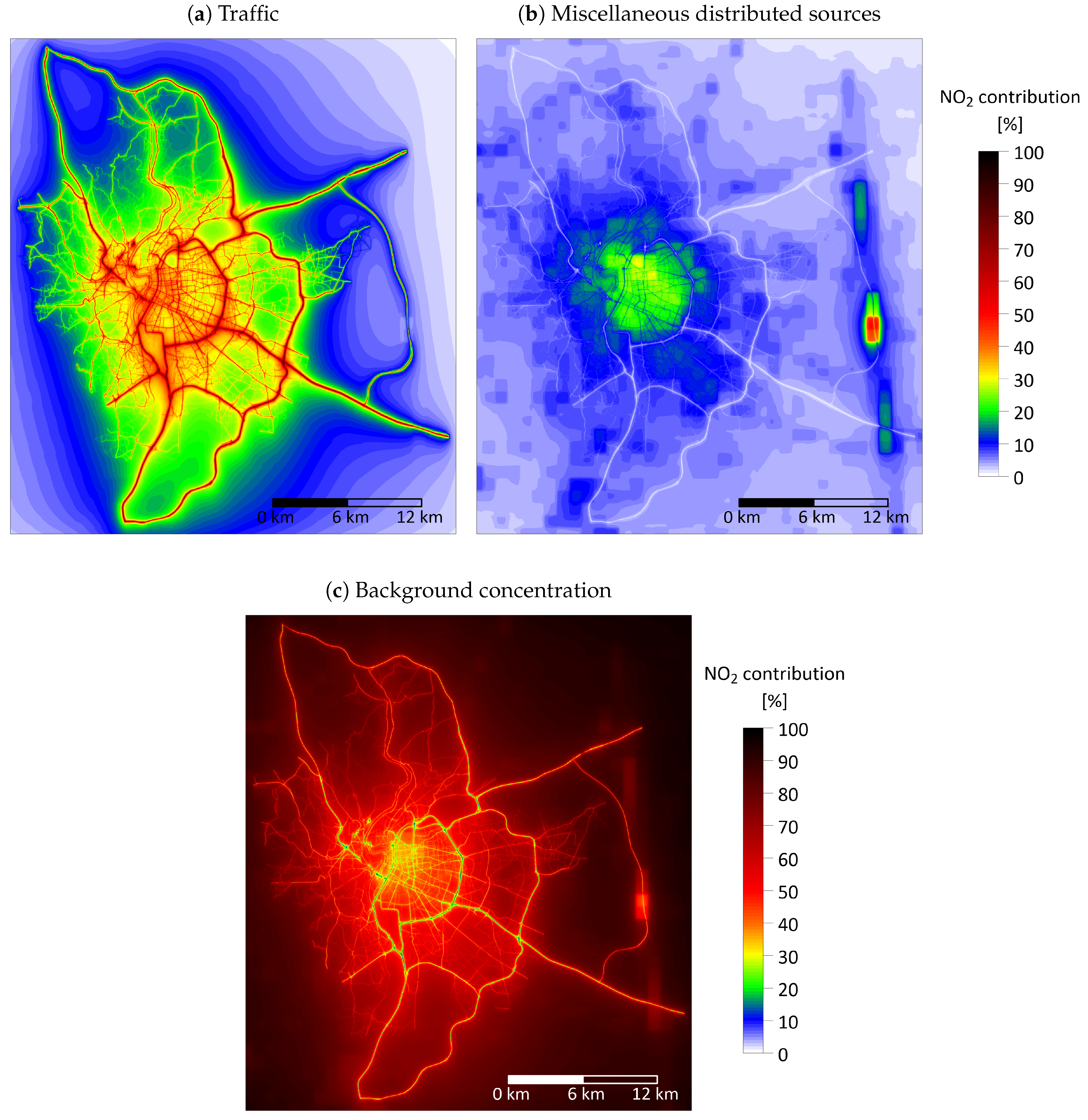
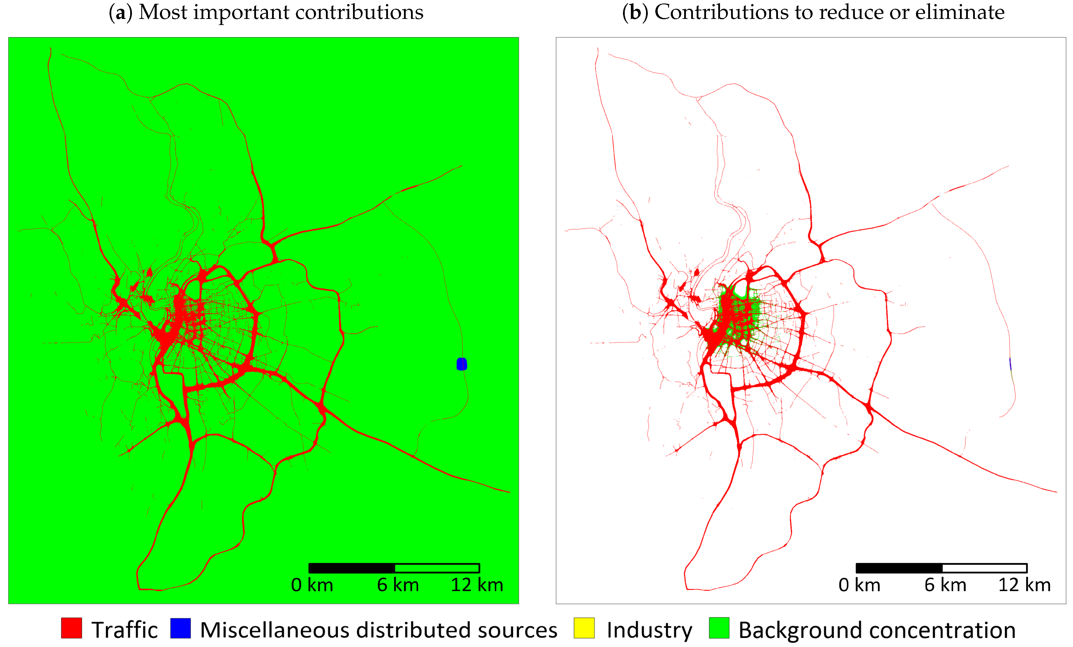
3.1.2. Estimates of Sources’ Contributions

Results show that the industrial sources’ contributions to NO₂ mean concentration are very low over the Lyon agglomeration. Those of the miscellaneous distributed sources are generally larger in the city centre (on average $6.42$ $\mathsf{\mu }$g m⁻³) (Figure 3). Results also show that the traffic contributions are on average higher close to the roads and in the centre of the agglomeration (Figure 3), where NO₂ traffic-induced concentrations can exceed the annual average concentration threshold set by the European Directive 2008/50/EC (40$\mathsf{\mu }$g m⁻³). Conversely, the background concentration contribution is at its lowest in the city centre and close to the main roads (on average $17.43$ $\mathsf{\mu }$g m⁻³).

The spatial variability of the relative contributions (on percentage) is different (Figure 5). The relative contribution of background concentration (on the total concentration) is globally larger than 50%, except close to some main roads (Figure 5c and Figure 6a). As expected, the traffic contribution is instead higher close to the roads, where its relative contribution exceeds 50% (Figure 5a and Figure 6a). For the miscellaneous distributed sources, the relative contribution is generally higher in the centre of the agglomeration, with some hot spot in the suburbs (Figure 5b). The industrial contribution is spatially homogeneous and relatively low (not shown in Figure 5).

The results of the source apportionment methods allow us to evaluate the contribution to the concentration registered at the monitoring station. We can therefore evaluate ex-post the pertinence of the classification of the monitoring stations adopted by the local air quality authority Atmo AURA. This classification is fully adapted for traffic-type and background-type stations, at which traffic and background contributions, respectively, both exceed 50% (Figure 4). Note also that the industrial, traffic, and miscellaneous distributed sources’ contributions are very low for the Saint-Exupéry station, which is therefore representative for the background concentration values.

A main objective of this kind of analysis is to identify sources having the main impacts on air quality and determine to what extent their emissions have to be reduced in order to attain given concentration threshold. As an example, we show in Figure 6b the contribution(s) to be reduced to lower concentrations below regulatory threshold values. These are determined by successively removing the different contributions, from the largest to the lowest, until reaching a concentration below the threshold value. The analysis suggests that the priority is to reduce the traffic emissions and, to a lesser extent, the emissions from sources placed outside the Lyon urban area (i.e., outside the domain taken into account this simulation), responsible for the background pollution.

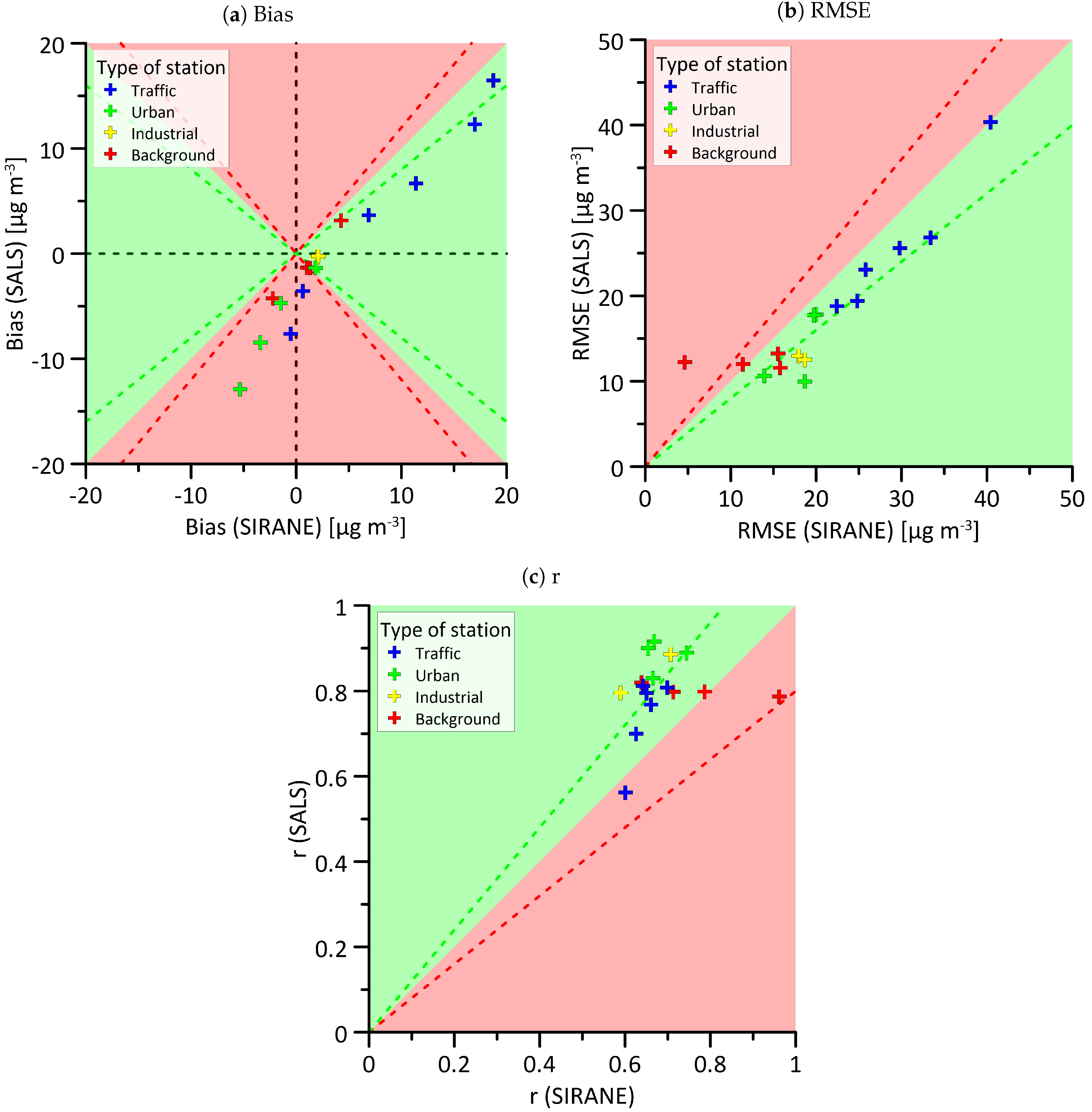
3.2. Data Assimilation Results

The SALS method is here applied using three groups of sources: (1) traffic emissions, (2) miscellaneous distributed sources and (3) background concentration and industrial sources.

To evaluate the performances of the method, we compare its results to those provided by the reference simulation (without data assimilation), using the leave-one-out cross-validation approach (LOOCV). This consists of estimating the concentration at one station (at each time step) using all available measured concentrations, except for that associated to that particular station. This procedure is repeated for each of the monitoring stations. The final estimates are compared to the measured concentrations. To evaluate the quality of the model results, we use six statistical indices: the bias, the fractional bias, the root mean square error (RMSE), the normalized mean square error (NMSE), the correlation coefficient (r) and the factor 2 (FAC2) [79]. The definition of these statistical indices are described in

Table 1. Statistical indices and quality criteria used to evaluate results quality ($c_m$ is the measured concentration and $c_p$ is the predicted concentration).

	Bias	RMSE	r
Definition	$\overline{c_m-c_p}$	${\displaystyle \frac{\overline{{\left(c_m-c_p\right)}^2}}{\overline{c_m}\overline{c_p}}}$	${\displaystyle \frac{\overline{\left(c_m-\overline{c_m}\right)\left(c_p-\overline{c_p}\right)}}{\sqrt{\overline{{\left(c_m-\overline{c_m}\right)}^2}\overline{{\left(c_p-\overline{c_p}\right)}^2}}}}$
Criteria	$\left|\mathrm{Bias}\right|\le 0.33\overline{c_m}$	$\mathrm{RMSE}\le \overline{c_m}$	$\mathrm{r}\ge 0.60$
	FB	NMSE	FAC2
Definition	${\displaystyle \frac{2\left(\overline{c_m}-\overline{c_p}\right)}{\overline{c_m}+\overline{c_p}}}$	${\displaystyle \frac{\overline{{\left(c_m-c_p\right)}^2}}{\overline{c_m}\overline{c_p}}}$	Fraction of data that satisfy $0.5\le c_m/c_p\le 2$
Criteria	$\left|\mathrm{FB}\right|\le 0.67$	$\mathrm{NMSE}\le 6$	$\mathrm{FAC}2\ge 0.30$

, where $c_m$ is the measured concentration and $c_p$ is the predicted concentration.

The statistical performances associated to the SALS method are given in

Table 2. Statistical performances of the SALS method ($\overline{c_m}$: mean measured concentration, $\overline{c_p}$: mean modelled concentration). Red values are those that do not respect the quality criteria.

Type	Station	$\overline{{\mathit{c}}_{\mathit{m}}}$	$\overline{{\mathit{c}}_{\mathit{p}}}$	Bias	FB	RMSE	NMSE	r	FAC2
		($\mathsf{\mu }$g m${}^{-3}$)	($\mathsf{\mu }$g m${}^{-3}$)	($\mathsf{\mu }$g m${}^{-3}$)		($\mathsf{\mu }$g m${}^{-3}$)
Traffic	A7	79.05	72.39	6.66	0.09	40.33	0.28	0.56	0.79
	BER	52.50	60.14	$-7.64$	$-0.14$	18.77	0.11	0.81	0.92
	GAR	74.06	61.78	12.28	0.18	26.80	0.16	0.81	0.95
	GC	47.06	43.41	3.65	0.08	19.39	0.18	0.79	0.90
	LP	50.67	54.26	$-3.59$	$-0.07$	23.04	0.19	0.70	0.87
	VAI	59.10	42.63	16.47	0.32	25.60	0.26	0.77	0.82
Urban	GER	38.08	39.47	$-1.39$	$-0.04$	9.95	0.07	0.91	0.96
	LC	37.95	50.87	−12.92	$-0.29$	17.82	0.16	0.90	0.87
	STJ	36.78	45.27	$-8.48$	$-0.21$	17.88	0.19	0.83	0.89
	VeV	26.67	31.39	$-4.72$	$-0.16$	10.61	0.13	0.89	0.82
Industrial	FEY	33.84	34.23	$-0.39$	$-0.01$	12.94	0.14	0.80	0.89
	STF	35.35	35.59	$-0.24$	$-0.01$	12.50	0.12	0.88	0.93
Background	COT	23.26	24.59	$-1.33$	$-0.06$	11.98	0.25	0.80	0.73
	GEN	33.36	34.73	$-1.37$	$-0.04$	13.22	0.15	0.80	0.86
	STE	17.78	22.04	$-4.26$	$-0.21$	12.21	0.38	0.79	0.64
	TER	29.41	26.27	3.14	0.11	11.57	0.17	0.82	0.83

. For all stations, statistical performances are good, except for the stations named A7 south Lyon (A7) and Lyon center (LC) (see Figure 1a), at which the correlation coefficient (or the bias) does not satisfy the quality criteria.

The bias, the RMSE and the correlation coefficients (r) of the SALS method are compared with those of the reference simulation in Figure 7. The bias of the SALS method is better than that associated to the reference simulation for half of the stations. Moreover, the absolute value of the least satisfactory bias is similar, with and without data assimilation. The RMSE values of the SALS method are generally better than those related to the reference simulation. However, the worst RMSE is of the same order of magnitude, with and without data assimilation. Similarly, the correlation coefficients associated with the SALS method are better than those related to the reference SIRANE simulation for most of the stations. Note, however, that the worst correlation coefficient does not vary significantly, with and without the application of the SALS method. Note that the bias, evaluated both before and after data assimilation, is generally negative for urban and background stations, therefore revealing a tendency of the model in overpredicting concentrations. This overprediction can be, at least partially, explained by the fact that SIRANE neglects the role of NO₂ losses induced by the reactions induced by the hydroxyl radical OH (Equation (4)).

4. Conclusions

A source apportionment module, using the tagged species approach, has been developed for the SIRANE model in order to estimate the contribution to air pollution of different typologies of pollutant sources. This module includes two methods, named SA-NO and SA-NOX, to evaluate the sources’ contributions to NO₂ concentrations. This module has been applied to evaluate the traffic, miscellaneous distributed sources including residential-tertiary sector, industrial sources and background concentration contribution to NO₂ concentration on the Lyon agglomeration in 2008. Overall, the NO₂ contributions evaluated with the SA-NO and SA-NOX models are similar. The contribution of the industrial sources to the NO₂ annual mean concentrations on the Lyon agglomeration is negligible compared to the other emissions’ sectors.The traffic emissions are instead the most important contributors. Their reduction is therefore essential to attain the threshold values set by the European regulations on air quality. The evaluation of the sources’ contributions allows also for an improvement of the urban air quality simulations’ results by means of the data assimilation method called Source Apportionment Least Square (SALS). Results highlight usefulness of the source apportionment method as a tool for the assessment of emissions reduction strategies at the local urban scale.

References

1. Wagstrom, K.M.; Pandis, S.N.; Yarwood, G.; Wilson, G.M.; Morris, R.E. Development and application of a computationally efficient particulate matter apportionment algorithm in a three-dimensional chemical transport model. Atmos. Environ. 2008, 42, 5650–5659. [Google Scholar] [CrossRef]
2. Yim, S.H.; Fung, J.C.; Lau, A.K. Use of high-resolution MM5/CALMET/CALPUFF system: SO2 apportionment to air quality in Hong Kong. Atmos. Environ. 2010, 44, 4850–4858. [Google Scholar] [CrossRef]
3. Cho, S.; Morris, R.; McEachern, P.; Shah, T.; Johnson, J.; Nopmongcol, U. Emission sources sensitivity study for ground-level ozone and PM2.5 due to oil sands development using air quality modelling system: Part II—Source apportionment modelling. Atmos. Environ. 2012, 55, 542–556. [Google Scholar] [CrossRef]
4. Grewe, V.; Dahlmann, K.; Matthes, S.; Steinbrecht, W. Attributing ozone to NOx emissions: Implications for climate mitigation measures. Atmos. Environ. 2012, 59, 102–107. [Google Scholar] [CrossRef] [Green Version]
5. Kwok, R.; Napelenok, S.; Baker, K. Implementation and evaluation of PM2.5 source contribution analysis in a photochemical model. Atmos. Environ. 2013, 80, 398–407. [Google Scholar] [CrossRef]
6. Ying, Q.; Kleeman, M.J. Source contributions to the regional distribution of secondary particulate matter in California. Atmos. Environ. 2006, 40, 736–752. [Google Scholar] [CrossRef]
7. Yarwood, G.; Morris, R.E.; Wilson, G.M. Particulate matter source apportionment technology (PSAT) in the CAMx photochemical grid model. In Air Pollution Modeling and Its Application XVII; Springer: Boston, MA, USA, 2007; pp. 478–492. [Google Scholar]
8. Wang, Z.S.; Chien, C.J.; Tonnesen, G.S. Development of a tagged species source apportionment algorithm to characterize three-dimensional transport and transformation of precursors and secondary pollutants. J. Geophys. Res. Atmos. 2009, 114. [Google Scholar] [CrossRef]
9. Pio, C.A.; Alves, C.A.; Duarte, A.C. Identification, abundance and origin of atmospheric organic particulate matter in a Portuguese rural area. Atmos. Environ. 2001, 35, 1365–1375. [Google Scholar] [CrossRef]
10. Querol, X.; Alastuey, A.; Rodríguez, S.; Plana, F.; Ruiz, C.R.; Cots, N.; Massagué, G.; Puig, O. PM10 and PM2.5 source apportionment in the Barcelona Metropolitan area, Catalonia, Spain. Atmos. Environ. 2001, 35, 6407–6419. [Google Scholar] [CrossRef]
11. Putaud, J.P.; Raes, F.; Van Dingenen, R.; Brüggemann, E.; Facchini, M.C.; Decesari, S.; Fuzzi, S.; Gehrig, R.; Hüglin, C.; Laj, P.; et al. A European aerosol phenomenology—2: Chemical characteristics of particulate matter at kerbside, urban, rural and background sites in Europe. Atmos. Environ. 2004, 38, 2579–2595. [Google Scholar] [CrossRef]
12. Gijzen, M.; Lewinsohn, E.; Savage, T.J.; Croteau, R.B. Conifer monoterpenes: Biochemistry and bark beetle chemical ecology. ACS Symp. Ser. 1993, 525, 8–22. [Google Scholar]
13. Watson, J.G. Overview of receptor model principles. J. Air Pollut. Control Assoc. 1984, 34, 619–623. [Google Scholar] [CrossRef]
14. Viana, M.; Kuhlbusch, T.; Querol, X.; Alastuey, A.; Harrison, R.; Hopke, P.; Winiwarter, W.; Vallius, M.; Szidat, S.; Prévôt, A.; et al. Source apportionment of particulate matter in Europe: A review of methods and results. J. Aerosol Sci. 2008, 39, 827–849. [Google Scholar] [CrossRef]
15. Held, T.; Ying, Q.; Kleeman, M.J.; Schauer, J.J.; Fraser, M.P. A comparison of the UCD/CIT air quality model and the CMB source–receptor model for primary airborne particulate matter. Atmos. Environ. 2005, 39, 2281–2297. [Google Scholar] [CrossRef]
16. Subramanian, R.; Donahue, N.M.; Bernardo-Bricker, A.; Rogge, W.F.; Robinson, A.L. Contribution of motor vehicle emissions to organic carbon and fine particle mass in Pittsburgh, Pennsylvania: Effects of varying source profiles and seasonal trends in ambient marker concentrations. Atmos. Environ. 2006, 40, 8002–8019. [Google Scholar] [CrossRef]
17. Rizzo, M.J.; Scheff, P.A. Fine particulate source apportionment using data from the USEPA speciation trends network in Chicago, Illinois: Comparison of two source apportionment models. Atmos. Environ. 2007, 41, 6276–6288. [Google Scholar] [CrossRef]
18. Subramanian, R.; Donahue, N.M.; Bernardo-Bricker, A.; Rogge, W.F.; Robinson, A.L. Insights into the primary–secondary and regional–local contributions to organic aerosol and PM2.5 mass in Pittsburgh, Pennsylvania. Atmos. Environ. 2007, 41, 7414–7433. [Google Scholar] [CrossRef]
19. Duvall, R.M.; Norris, G.A.; Burke, J.M.; Olson, D.A.; Vedantham, R.; Williams, R. Determining spatial variability in PM2.5 source impacts across Detroit, MI. Atmos. Environ. 2012, 47, 491–498. [Google Scholar] [CrossRef]
20. Guo, H.; Wang, T.; Louie, P. Source apportionment of ambient non-methane hydrocarbons in Hong Kong: Application of a principal component analysis/absolute principal component scores (PCA/APCS) receptor model. Environ. Pollut. 2004, 129, 489–498. [Google Scholar] [CrossRef] [PubMed]
21. Almeida, S.M.; Pio, C.A.; Freitas, M.C.; Reis, M.A.; Trancoso, M.A. Approaching PM2.5 and PM2.5–10 source apportionment by mass balance analysis, principal component analysis and particle size distribution. Sci. Total Environ. 2006, 368, 663–674. [Google Scholar] [CrossRef] [PubMed]
22. Song, Y.; Xie, S.; Zhang, Y.; Zeng, L.; Salmon, L.G.; Zheng, M. Source apportionment of PM2.5 in Beijing using principal component analysis/absolute principal component scores and UNMIX. Sci. Total Environ. 2006, 372, 278–286. [Google Scholar] [CrossRef] [PubMed]
23. Shi, G.L.; Li, X.; Feng, Y.C.; Wang, Y.Q.; Wu, J.H.; Li, J.; Zhu, T. Combined source apportionment, using positive matrix factorization–chemical mass balance and principal component analysis/multiple linear regression–chemical mass balance models. Atmos. Environ. 2009, 43, 2929–2937. [Google Scholar] [CrossRef]
24. Escrig, A.; Monfort, E.; Celades, I.; Querol, X.; Amato, F.; Minguillón, M.C.; Hopke, P.K. Application of Optimally Scaled Target Factor Analysis for Assessing Source Contribution of Ambient PM10. J. Air Waste Manag. Assoc. 2009, 59, 1296–1307. [Google Scholar] [CrossRef] [PubMed]
25. Minguillón, M.C.; Schembari, A.; Triguero-Mas, M.; de Nazelle, A.; Dadvand, P.; Figueras, F.; Salvado, J.A.; Grimalt, J.O.; Nieuwenhuijsen, M.; Querol, X. Source apportionment of indoor, outdoor and personal PM2.5 exposure of pregnant women in Barcelona, Spain. Atmos. Environ. 2012, 59, 426–436. [Google Scholar] [CrossRef]
26. Alier, M.; Felipe-Sotelo, M.; Hernàndez, I.; Tauler, R. Variation patterns of nitric oxide in Catalonia during the period from 2001 to 2006 using multivariate data analysis methods. Anal. Chim. Acta 2009, 642, 77–88. [Google Scholar] [CrossRef] [PubMed]
27. Alier, M.; Felipe, M.; Hernández, I.; Tauler, R. Trilinearity and component interaction constraints in the multivariate curve resolution investigation of NO and O3 pollution in Barcelona. Anal. Bioanal. Chem. 2011, 399, 2015–2029. [Google Scholar] [CrossRef] [PubMed]
28. Koo, B.; Wilson, G.M.; Morris, R.E.; Dunker, A.M.; Yarwood, G. Comparison of source apportionment and sensitivity analysis in a particulate matter air quality model. Environ. Sci. Technol. 2009, 43, 6669–6675. [Google Scholar] [CrossRef] [PubMed]
29. Hendriks, C.; Kranenburg, R.; Kuenen, J.; van Gijlswijk, R.; Kruit, R.W.; Segers, A.; van der Gon, H.D.; Schaap, M. The origin of ambient particulate matter concentrations in the Netherlands. Atmos. Environ. 2013, 69, 289–303. [Google Scholar] [CrossRef]
30. Grewe, V. A diagnostic for ozone contributions of various NOx emissions in multi-decadal chemistry-climate model simulations. Atmos. Chem. Phys. 2004, 4, 729–736. [Google Scholar] [CrossRef]
31. Held, T.; Ying, Q.; Kaduwela, A.; Kleeman, M. Modeling particulate matter in the San Joaquin Valley with a source-oriented externally mixed three-dimensional photochemical grid model. Atmos. Environ. 2004, 38, 3689–3711. [Google Scholar] [CrossRef]
32. Grewe, V.; Tsati, E.; Hoor, P. On the attribution of contributions of atmospheric trace gases to emissions in atmospheric model applications. Geosci. Model Dev. 2010, 3, 487. [Google Scholar] [CrossRef] [Green Version]
33. Butler, T.; Lawrence, M.; Taraborrelli, D.; Lelieveld, J. Multi-day ozone production potential of volatile organic compounds calculated with a tagging approach. Atmos. Environ. 2011, 45, 4082–4090. [Google Scholar] [CrossRef]
34. Emmons, L.; Hess, P.; Lamarque, J.F.; Pfister, G. Tagged ozone mechanism for MOZART-4, CAM-chem and other chemical transport models. Geosci. Model Dev. 2012, 5, 1531. [Google Scholar] [CrossRef]
35. Kranenburg, R.; Segers, A.; Hendriks, C.; Schaap, M. Source apportionment using LOTOS-EUROS: Module description and evaluation. Geosci. Model Dev. 2013, 6, 721–733. [Google Scholar] [CrossRef]
36. Granier, C.; Mueller, J.; Pétron, G.; Brasseur, G. A three-dimensional study of the global CO budget. Chemosphere-Glob. Chang. Sci. 1999, 1, 255–261. [Google Scholar] [CrossRef]
37. Granier, C.; Pétron, G.; Müller, J.F.; Brasseur, G. The impact of natural and anthropogenic hydrocarbons on the tropospheric budget of carbon monoxide. Atmos. Environ. 2000, 34, 5255–5270. [Google Scholar] [CrossRef]
38. Lamarque, J.F.; Hess, P. Model analysis of the temporal and geographical origin of the CO distribution during the TOPSE campaign. J. Geophys. Res. Atmos. 2003, 108. [Google Scholar] [CrossRef]
39. Pfister, G.; Petron, G.; Emmons, L.; Gille, J.; Edwards, D.; Lamarque, J.F.; Attie, J.L.; Granier, C.; Novelli, P. Evaluation of CO simulations and the analysis of the CO budget for Europe. J. Geophys. Res. Atmos. 2004, 109. [Google Scholar] [CrossRef]
40. Huang, Q.; Cheng, S.; Perozzi, R.E.; Perozzi, E.F. Use of a MM5–CAMx–PSAT modeling system to study SO2 source apportionment in the Beijing Metropolitan Region. Environ. Model. Assess. 2012, 17, 527–538. [Google Scholar] [CrossRef]
41. Talagrand, O. Assimilation of observations, an introduction. J. Meteorol. Soc. Jpn. 1997, 75, 191–209. [Google Scholar] [CrossRef]
42. Rabier, F. Assimilation variationnelle de données météorologiques en présence d’instabilité barocline. La Météorologie 1993, 8, 57–72. [Google Scholar] [CrossRef]
43. Kalnay, E. Atmospheric Modeling, Data Assimilation and Predictability; Cambridge University Press: Cambridge, UK, 2003. [Google Scholar]
44. Swinbank, R.; Shutyaev, V.; Lahoz, W.A. Data Assimilation for the Earth System; Springer Science & Business Media: Berlin, Germany, 2003. [Google Scholar]
45. Denby, B.; Horálek, J.; Walker, S.E.; Eben, K.; Fiala, J. Interpolation and assimilation methods for European scale air quality assessment and mapping. In Part I: Review and Recommendations; European Topic Centre on Air and Climate Change (ETC/ACC): Copenhagen, Denmark, 2005; Volume 7. [Google Scholar]
46. Morel, P.; Talagrand, O. Dynamic approach to meteorological data assimilation. Tellus 1974, 26, 334–344. [Google Scholar] [CrossRef]
47. McPherson, R.D. Progress, problems, and prospects in meteorological data assimilation. Bull. Am. Meteorol. Soc. 1975, 56, 1154–1166. [Google Scholar] [CrossRef]
48. Miyakoda, K.; Umscheid, L.; Lee, D.; Sirutis, J.; Lusen, R.; Pratte, F. The near-real-time, global, four-dimensional analysis experiment during the GATE period, Part I. J. Atmos. Sci. 1976, 33, 561–591. [Google Scholar] [CrossRef]
49. Miyakoda, K.; Strickler, R.; Chludzinski, J. Initialization with the data assimilation method. Tellus 1978, 30, 32–54. [Google Scholar] [CrossRef]
50. McPherson, R.; Bergman, K.; Kistler, R.; Rasch, G.; Gordon, D. The NMC operational global data assimilation system. Mon. Weather Rev. 1979, 107, 1445–1461. [Google Scholar] [CrossRef]
51. Elbern, H.; Schmidt, H.; Ebel, A. Variational data assimilation for tropospheric chemistry modeling. J. Geophys. Res. Atmos. 1997, 102, 15967–15985. [Google Scholar] [CrossRef]
52. Elbern, H.; Schmidt, H. A four-dimensional variational chemistry data assimilation scheme for Eulerian chemistry transport modeling. J. Geophys. Res. Atmos. 1999, 104, 18583–18598. [Google Scholar] [CrossRef]
53. Elbern, H.; Schmidt, H.; Talagrand, O.; Ebel, A. 4D-variational data assimilation with an adjoint air quality model for emission analysis. Environ. Model. Softw. 2000, 15, 539–548. [Google Scholar] [CrossRef]
54. Segers, A.J.; Heemink, A.W.; Verlaan, M.; van Loon, M. A modified rrsqrt-filter for assimilating data in atmospheric chemistry models. Environ. Model. Softw. 2000, 15, 663–671. [Google Scholar] [CrossRef]
55. Van Loon, M.; Builtjes, P.J.H.; Segers, A.J. Data assimilation of ozone in the atmospheric transport chemistry model LOTOS. Environ. Model. Softw. 2000, 15, 603–609. [Google Scholar] [CrossRef]
56. Brown, D.; Comrie, A. Spatial modeling of winter temperature and precipitation in Arizona and New Mexico, USA. Clim. Res. 2002, 22, 115–128. [Google Scholar] [CrossRef]
57. Hooyberghs, J.; Mensink, C.; Dumont, G.; Fierens, F. Spatial interpolation of ambient ozone concentrations from sparse monitoring points in Belgium. J. Environ. Monit. 2006, 8, 1129–1135. [Google Scholar] [CrossRef] [PubMed]
58. ETC/ACC. Spatial Mapping of Air Quality for European Scale Assessment; ETC/ACC: Copenhagen, Denmark, 2007. [Google Scholar]
59. Lü, C.; Tian, H. Spatial and temporal patterns of nitrogen deposition in China: Synthesis of observational data. J. Geophys. Res. D Atmos. 2007, 112. [Google Scholar] [CrossRef]
60. Denby, B.; Schaap, M.; Segers, A.; Builtjes, P.; Horálek, J. Comparison of two data assimilation methods for assessing PM10 exceedances on the European scale. Atmos. Environ. 2008, 42, 7122–7134. [Google Scholar] [CrossRef]
61. EEA. Spatial Assessment of PM10 and Ozone Concentrations in Europe (2005); European Environment Agency (EEA): Copenhagen, Denmark, 2009. [Google Scholar]
62. Joseph, J.; Sharif, H.O.; Sunil, T.; Alamgir, H. Application of validation data for assessing spatial interpolation methods for 8-h ozone or other sparsely monitored constituents. Environ. Pollut. 2013, 178, 411–418. [Google Scholar] [CrossRef] [PubMed]
63. Blanchard, C.L.; Tanenbaum, S.; Hidy, G.M. Spatial and temporal variability of air pollution in Birmingham, Alabama. Atmos. Environ. 2014, 89, 382–391. [Google Scholar] [CrossRef]
64. Candiani, G.; Carnevale, C.; Pisoni, E.; Volta, M. Assimilation of Chemical Ground Measurements in Air Quality Modeling. In Large-Scale Scientific Computing; Lirkov, I., Margenov, S., Waśniewski, J., Eds.; Springer: Berlin/Heidelberg, Germany, 2010; pp. 157–164. [Google Scholar]
65. Wang, X.; Mallet, V.; Berroir, J.P.; Herlin, I. Assimilation of OMI NO2 retrievals into a regional chemistry-transport model for improving air quality forecasts over Europe. Atmos. Environ. 2011, 45, 485–492. [Google Scholar] [CrossRef]
66. Kumar, U.; De Ridder, K.; Lefebvre, W.; Janssen, S. Data assimilation of surface air pollutants (O3 and NO2) in the regional-scale air quality model AURORA. Atmos. Environ. 2012, 60, 99–108. [Google Scholar] [CrossRef]
67. Candiani, G.; Carnevale, C.; Finzi, G.; Pisoni, E.; Volta, M. A comparison of reanalysis techniques: Applying optimal interpolation and Ensemble Kalman Filtering to improve air quality monitoring at mesoscale. Sci. Total Environ. 2013, 458–460, 7–14. [Google Scholar] [CrossRef] [PubMed]
68. Tilloy, A.; Mallet, V.; Poulet, D.; Pesin, C.; Brocheton, F. BLUE-based NO2 data assimilation at urban scale. J. Geophys. Res. Atmos. 2013, 118, 2031–2040. [Google Scholar] [CrossRef] [Green Version]
69. Soulhac, L.; Salizzoni, P.; Cierco, F.X.; Perkins, R. The model SIRANE for atmospheric urban pollutant dispersion; part I, presentation of the model. Atmos. Environ. 2011, 45, 7379–7395. [Google Scholar] [CrossRef]
70. Soulhac, L.; Salizzoni, P.; Mejean, P.; Didier, D.; Rios, I. The model SIRANE for atmospheric urban pollutant dispersion; PART II, validation of the model on a real case study. Atmos. Environ. 2012, 49, 320–337. [Google Scholar] [CrossRef]
71. Soulhac, L. ModéLisation de la Dispersion Atmosphérique à L’intérieur de la Canopée Urbaine. Ph.D. Thesis, Ecole centrale de Lyon, Ecully, France, 2000. [Google Scholar]
72. Soulhac, L.; Nguyen, C.V.; Volta, P.; Salizzoni, P. The model SIRANE for atmospheric urban pollutant dispersion. PART III: Validation against NO2 yearly concentration measurements in a large urban agglomeration. Atmos. Environ. 2017, 167, 377–388. [Google Scholar] [CrossRef]
73. Seinfeld, J.H. Atmospheric Chemistry and Physics of Air Pollution, 1st ed.; Wiley-Interscience: New York, NY, USA, 1986. [Google Scholar]
74. Bloss, W. Atmospheric chemical processes of importance in cities. Issues Environ. Sci. Technol. 2009, 28, 42. [Google Scholar]
75. Zhong, J.; Cai, X.M.; Bloss, W.J. Modelling the dispersion and transport of reactive pollutants in a deep urban street canyon: Using large-eddy simulation. Environ. Pollut. 2015, 200, 42–52. [Google Scholar] [CrossRef] [PubMed]
76. Kasten, F.; Czeplak, G. Solar and terrestrial radiation dependent on the amount and type of cloud. Sol. Energy 1980, 24, 177–189. [Google Scholar] [CrossRef]
77. Vardoulakis, S.; Fisher, B.E.; Pericleous, K.; Gonzalez-Flesca, N. Modelling air quality in street canyons: A review. Atmos. Environ. 2003, 37, 155–182. [Google Scholar] [CrossRef]
78. Lawson, C.L.; Hanson, R. Linear least squares with linear inequality constraints. Chap 1974, 23, 158–173. [Google Scholar]
79. Hanna, S.; Chang, J. Acceptance criteria for urban dispersion model evaluation. Meteorol. Atmos. Phys. 2012, 116, 133–146. [Google Scholar] [CrossRef]
Figure 1. Localisation of the measurements and meteorology (Bron) stations (a); annual mean emissions of industries (b); traffic (c); and distributed miscellaneous sources (mainly domestic heating) (d).
Atmosphere 09 00008 g001
Figure 2. Annual statistics of data collected at the Bron meteorological station in 2008: (a) Windrose and (b) probability density function of the ratio 1/L MO .
Atmosphere 09 00008 g002
Figure 3. Traffic, miscellaneous distributed sources, background contribution ( μ g m−3) to the NO 2 annual mean concentration on the Lyon agglomeration in 2008 estimated with the SA-NO model (a,c,e) and SA-NOX (b,d,f) models (grey areas correspond to negative contributions).
Atmosphere 09 00008 g003
Figure 4. Traffic, miscellaneous distributed sources, industry, and background contribution ( μ g m−3) to the NO 2 annual mean concentration at the measurement station located in the Lyon agglomeration in 2008 estimated with the SA-NO (left bars) and the SA-NOX (right-handed bars) models.
Atmosphere 09 00008 g004
Figure 5. (a) Traffic, (b) miscellaneous distributed sources, and (c) background relative contribution [%] to the NO 2 annual mean concentration on the Lyon agglomeration in 2008 estimated with the SA-NOX model.
Atmosphere 09 00008 g005
Figure 6. Map of (a) the most important NO 2 contributor on the Lyon urban area in 2008 and (b) the NO 2 contributions to reduce or eliminate in order to achieve air quality European standard in 2008 (the concentration is (already) below the threshold value in area in white).
Atmosphere 09 00008 g006
Figure 7. (a) Bias, (b) RMSE, and (c) correlation coefficients before and after data assimilation (the green zone indicates results improved after data assimilation and the red region indicates results worsened after data assimilation. Green (red) dot line indicates improvement (worsening) of 20% after data assimilation).
Atmosphere 09 00008 g007