Abstract
Previous researchers calculated air change rate per hour (ACH) in the urban canopy layers (UCL) by integrating the normal component of air mean velocity (convection) and fluctuation velocity (turbulent diffusions) across UCL boundaries. However they are usually greater than the actual ACH induced by flow rates flushing UCL and never returning again. As a novelty, this paper aims to verify the exponential concentration decay history occurring in UCL models and applies the concentration decay method to assess the actual UCL ACH and predict the urban age of air at various points. Computational fluid dynamic (CFD) simulations with the standard k-ε models are successfully validated by wind tunnel data. The typical street-scale UCL models are studied under neutral atmospheric conditions. Larger urban size attains smaller ACH. For square overall urban form (Lx = Ly = 390 m), the parallel wind (θ = 0°) attains greater ACH than non-parallel wind (θ = 15°, 30°, 45°), but it experiences smaller ACH than the rectangular urban form (Lx = 570 m, Ly = 270 m) under most wind directions (θ = 30° to 90°). Open space increases ACH more effectively under oblique wind (θ = 15°, 30°, 45°) than parallel wind. Although further investigations are still required, this paper provides an effective approach to quantify the actual ACH in urban-like geometries.
1. Introduction
The increase in number of vehicles in cities and the ongoing urbanization worldwide are causing more concerns about urban air pollution. The urban canopy layer (UCL) is defined as the outdoor air volume below the rooftops of buildings [1]. Raising UCL ventilation capacity by the surrounding atmosphere with relatively clean air has been regarded as one effective approach to diluting environmental pollutants [2,3,4,5,6,7,8] and improving the urban thermal environment in the hot summer [9,10] as well as reducing human exposure to outdoor pollutants [11,12,13].
UCL ventilation is strongly correlated to urban morphologies. For two-dimensional street canyons [14,15,16,17,18,19], street aspect ratio (building height/street width, H/W) is the first key parameter to affect the flow regimes and UCL ventilation. Four flow regimes have been classified depending on different aspect ratios (H/W) [14,15,16], i.e., the isolated roughness flow regime (IRF, in which the aspect ratio is less than 0.1 to 0.125), the wake interference flow regime (WIF, with an aspect ratio of 0.1 to 0.67), the skimming flow regime (SF, with an aspect ratio of 0.67 to 1.67), and the multi-vortex regime in two-dimensional deep street canyons with two or more vortices as H/W > 1.67. For three-dimensional UCL geometries, the plan area index λp and frontal area index λf [4,5,6,9,10] are regarded as the key urban parameters to influence the flow and pollutant dispersion in urban areas. In addition, the other factors including overall urban form and ambient wind directions [2,3,6,7,8,9], building height variations [5,20,21,22,23,24,25], thermal buoyancy force for weak-wind atmospheric conditions [10,18,26,27,28,29,30], etc. also play significant roles in the flow and pollutant dispersion in UCL models.
In recent years, various ventilation indices have been applied for UCL ventilation assessment, such as pollutant retention time and purging flow rate [2,7,23], age of air and ventilation efficiency [3,4,5,6,7,23], in-canopy velocity and exchange velocity [22,25], net escape velocity [31], etc. Similar to indoor ventilation [32,33,34,35,36], the key point of applying these ventilation indices is based on the UCL ventilation processes as below: The surrounding external air is relatively clean and can be transported into urban areas to aid pollutant dilution with physical processes of horizontal dilution, vertical transport, recirculation of contaminants, and turbulent diffusion. In this sense, the tracer gas technique originated from indoor ventilation sciences has been used to predict outdoor ventilation by analyzing the final steady-state pollutant concentrations or the transient concentration decay history, which illustrates the processes of pollutant dilution and ventilation. For example, the concept of purging flow rate (PFR) was adopted to assess the net flow rate of flushing the urban domain [2] or the entire urban canopy layer [23] induced by the convection and turbulent diffusion. Moreover, the urban age of air [3,4,5,6,7] represents how long the external air can reach a place after it enters the UCL space. Hang et al. [3] first adopted the homogeneous emission method into CFD simulations [32] to calculate the urban age of air for quantifying the characteristics of wind supplying external air into UCL space for pollutant dilution.
In particular, the air change rate per hour is one of the most widely used indoor ventilation concepts [32,33,34,35,36], calculated by ACH = 3600QT/Vol, where QT is the total volumetric flow rate and Vol is the room volume. Later it is adopted to quantify the volumetric air exchange rate of the entire UCL volume per hour, including two-dimensional street canyon ventilation assessment [37,38] and three-dimensional UCL ventilation modeling [39,40,41,42,43,44]. Previous researchers usually calculated outdoor ACH indexes based on the volumetric flow rate obtained by integrating the mean value of the component of the mean velocity normal to the UCL boundaries and the effective flow rate due to turbulence based on integrating half the standard deviation (rms-value) of the velocity fluctuations on street roofs [37,38,39,40,41,42,43,44]. Specially, vertical turbulent exchange across a street roof has been verified to significantly influence UCL ventilation and pollutant removal in urban-like geometries [37,38,39,40] because street roofs are open at the top with a large area. However, the mean velocity often exhibits recirculation and the velocity fluctuations across the UCL open roof are bidirectional and therefore air or pollutant can return to the given UCL space several times. Thus, these two ACH indexes do not represent the entire UCL air volume that is really exchanged ACH times in an hour by external air, i.e., they are not the actual air change rate per hour in UCL models calculated by the actual flow rate flushing or leaving this space and never returning again. There are efficiency problems in UCL ventilation assessment [3,5].
The purpose of this paper is to predict the actual or net air change rate per hour in UCL models and how it is related to urban morphologies and atmospheric conditions. The net or actual air change rate is defined as the exchange of air flushing the space and never returning to the UCL space again. It depends on several time scales, i.e., the overall turn over time (air volume (Vol) divided by the total volumetric flow rate (QT)), purging time for air moving from entrances to exits, time constant for local vortices and turbulent mixing. The concentration decay method has been widely used to predict the actual ACH and age of air in indoor environments in which the concentration temporal profile accords with the exponential decay law and the concentration decay history shows the pollutant dilution and ventilation processes in room ventilation [32,33,34,35,36,45,46]. However, to date, this method has not been introduced to quantify the actual or net ACH index and age of air in UCL models.
Therefore, as a novelty, this paper aims to verify whether the temporal decay profile of concentration in UCL models accords with the exponential decay law and explore the effectiveness of applying concentration decay method for outdoor ventilation assessment. As a start, the typical medium-dense urban canopy layers (H/W = 1, λf = λp = 0.25) are first studied. The effects of urban size, ambient wind directions, overall urban forms, and open space arrangements are evaluated under neutral atmospheric conditions.
2. Methodology
2.1. Turbulence Models for Urban Airflow Modeling
As outlined by the review papers, CFD simulations have been widely applied in urban flow/dispersion modeling outdoor in the last two decades [47,48,49]. Large eddy simulations (LES) are known to perform better in predicting turbulence than the Reynolds-Averaged Navier-Stokes (RANS) approaches. However, there are still some challenges involved with widely applying LES because of the strongly increased computational requirements, the development of advanced sub-grid scale models, and the difficulty in specifying appropriate time-dependent inlet and wall boundary conditions [16,17,20,26,38,39]. Therefore, in quantitative work one has to adopt time-averaged turbulence models (i.e., RANS approaches). Actually, in spite of their deficiencies in predicting turbulence, steady RANS models have become the most popular CFD approaches for urban flow modeling, and the standard k-ε model is one of the most widely adopted in the literature [2,3,5,6,7,9,10,11,21,22,23], with successful validation by wind tunnel measurements and good performance in predicting mean flows. This paper selects the standard k-ε model and the CFD validation case is conducted to evaluate the reliability of CFD methodologies by wind tunnel data.
2.2. Model Description in the CFD Validation Case
As shown in Figure 1a, Brown et al. [50] measured turbulent airflows in a seven-row and 11-column cubic building array with a parallel approaching wind. Building width (B), building height (H), and street width (W) are the same (B = H = W = 15 cm, H/W = 1, building packing densities λp = λf = 0.25, Lx = 13H, Ly = 21H). The scale ratio to full-scale models is 1:200. x, y, and z are the stream-wise, span-wise (lateral), and vertical directions. x/H = 0 represents the location of windward street opening. y/H = 0 is the vertical symmetric plane of the middle column. Point Vi represents the center point of the secondary street No. i. The measured vertical profiles of time-averaged (or mean) velocity components (stream-wise velocity , vertical velocity ), and turbulence kinetic energy at Points Vi are used to evaluate CFD simulations.
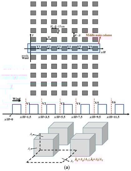
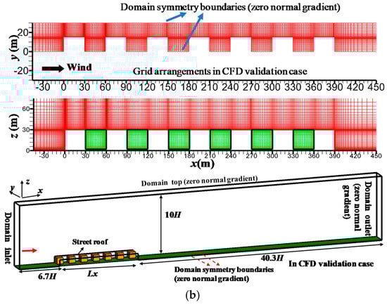
Figure 1.
(a) Model description of wind tunnel test; (b) setups in CFD validation case.
In the CFD validation case, the full-scale seven-row building array is numerically investigated (B = H = W = 30 m, λp = λf = 0.25, H/W = 1; see Figure 1b). According to the literature [23,51,52,53], the lateral urban boundaries hardly affect airflows in the middle column as the wind tunnel model is sufficiently wide in the lateral (y) direction (Ly = 21H). Thus, it is effective to only consider half of this middle column (shaded area in Figure 1a) to reduce the computational requirement. Figure 1b shows model geometry, grid arrangements, CFD domain, and boundary conditions. In particular, the distances of UCL boundaries to the domain inlet, domain outlet, and domain top are 6.7H, 40.3H, and 9.0H, respectively. Zero normal gradient condition is used at the domain top, domain outlet, and two lateral domain symmetry boundaries. At the domain inlet, the measured power-law profile of time-averaged (or mean) velocity U0(z) in the upstream free flow is adopted (see Equation (1a)) (Brown et al. [51]). Moreover, the vertical profiles of turbulent kinetic energy k(z) and its dissipation rate (ε) at the domain inlet are calculated by Equations (1b) and (1c) [23,51,52,53]:
where Uref (=3.0 ms−1) is the reference velocity at the building height (H = 30 m), is a constant (=0.09), u* is the friction velocity (=0.24 ms−1), and is von Karman’s constant (=0.41).
For this CFD validation case, hexahedral cells of 531,657 and the minimum cell sizes of 0.5 m (H/60) are used (the medium grid). Following the CFD guidelines [54,55], four hexahedral cells exist below the pedestrian level (z = 0 m to 2 m). The grid expansion ratio from wall surfaces to the surrounding is 1.15. With such grid arrangements, the normalized distance from wall surfaces y+ () ranges from 60 to 1000 at most regions of wall surfaces within UCL space.
No slip boundary condition with standard wall function [56] is used at wall surfaces. The practice guidelines for setting the upstream and downstream ground are followed to reproduce a horizontally homogeneous atmospheric boundary layer surrounding urban areas [46,57]: The roughness height kS and the roughness constant CS are correlated by the aerodynamic roughness length z0:
Note that the distance between the center point P of the ground adjacent cell and the ground surface is YP = 0.25 m. Fluent 6.3 does not allow kS to be larger than YP [57]. Thus, according to van Hooff and Blocken [46], a user-defined function is used to set the roughness constant CS = 4 because Fluent 6.3 does not allow it to be greater than 1. Then as CS = 4 and z0 = 0.1 m, kS = 0.245 m is smaller than YP = 0.25 m.
ANSYS FLUENT with the finite volume method is used to predict the steady isothermal urban airflows [56]. The SIMPLE scheme is adopted to couple the pressure to the velocity field. The first-order upwind scheme is not appropriate for all transported quantities since the spatial gradients of the quantities tend to become diffusive due to a large viscosity. Thus, as recommended by the literature [54,55], all transport equations are discretized by the second-order upwind scheme for better numerical accuracy. The under-relaxation factors for pressure term, momentum term, k, and ε terms are 0.3, 0.7, 0.5, and 0.5, respectively. The solutions do not stop until all residuals become constant. The fine grid with a minimum size of 0.2 m (H/150) is also adopted to perform a grid independence study. The above CFD settings on domain sizes, grid arrangements and boundary conditions fulfill the major requirements given by CFD guidelines [54,55]. In particular, steady CFD simulations are first carried out about 4000 iterations with the first-order upwind scheme, then continued with the second-order upwind scheme until all residuals became constant. The residuals reached the following minimum values or less: 10−4 for the continuity equation, 0.5 × 10⁻⁵ for the velocity components and k, 0.5 × 10⁻⁵ and 0.5 × 10⁻⁴ for pollutant concentration and ε. After solving the steady-state airflow field, the uniform initial concentration C(0) is defined in the entire urban canopy layer, then the unsteady concentration decay history is calculated and recorded for ventilation assessment as the solved flow field remains constant.
2.3. Model Description in All CFD Test Cases
As displayed in Table 1 and Figure 2a–d, two groups of medium-dense UCL models (H = B = W = 30 m, λp = λf = 0.25) are investigated in CFD simulations. The row and column numbers are referred to the numbers of buildings along the stream-wise direction (x, main streets) and span-wise direction (y, secondary streets). Wind directions are represented by the angles (θ = 0° to 90°) between the approaching wind and the main streets.

Table 1.
Test cases investigated ( = = 0.25, H/W = 1).
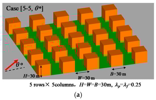
Figure 2.
(a) Model description and (b) computational domain of Case [5-5, 0°] (θ = 0°); (c) Computational domain in Case [5-5, θ] (θ =15°, 30°, 45°); (d) Model description of Case [5-5, θ, Oij]; (e) Definition of initial-state concentration field in the entire UCL space.
In Group I (Table 1 and Figure 2a), test cases without open space are named as Case [row number-column number, wind direction θ°]. For cases with a parallel approaching wind (θ = 0°, Figure 2b), three cases are included (i.e., Case [5-5, 0°], Case [7-7, 0°], Case [10-5, 0°]) with only half of computational domain simulated. The distances from UCL boundaries to the domain top, domain outlet, domain inlet, and the domain lateral boundary are 9H, 40.3H, 6.7H, and 10H, respectively. Zero normal gradient boundary condition is used at the domain outlet, domain top, and the lateral domain boundary. At the domain inlet, Equation (1) is used to provide the boundary condition.
For test cases with oblique wind (θ = 15°, 30°, 45°, 60°, 75°, 90°, Figure 2c), the full CFD domains are used. There are two domain inlets and two domain outlets. The distances from UCL boundaries to the domain top, domain outlets, domain inlets are 9H, 41H and 6.7H. At two domain inlets, the vertical profiles of time-averaged (or mean) velocity components in Equations (3a)–(3c) and turbulent quantities defined in Equations (1b) and (1c) are used to define boundary conditions:
At the domain outlets and domain top, the zero normal gradient boundaries are used.
In Group II (Table 1 and Figure 2d), for UCL models with five rows and five columns, open space arrangements are included. In total 24 test cases of Case [5-5, θ°, Oij] are investigated (θ = 0°, 15°, 30°, 45°). Here Oij represents only one building of position i-j (2-1, 2-2, 2-3, 2-4, 3-3, or 3-4) (see Figure 2d) is removed to attain an open space effect. Computational domain and boundary conditions are similar to Group I.
For all the test cases in Table 1, the grid arrangements are similar to the medium grid of the CFD validation case. The total number of hexahedral cells is from 531,657 to 3,360,096. The above CFD settings on domain sizes, grid arrangements, and boundary conditions fulfill the major requirements recommended by the best CFD guidelines.
2.4. ACH Indexes and Age of Air by Concentration Decay Method
2.4.1. Volumetric Flow Rates and the Corresponding ACH [23,37,38,39,40,41,42]
To analyze the flow field, the velocity components and wind speed are all normalized by the reference velocity in the upstream free flow at the same height, i.e., Equation (1a) at the domain inlet . For example, for velocity at z = 15 m = 0.5H, the velocity is normalized by dividing it by U0 (z = 15 m) = 2.685 ms−1.
To quantify the ventilation capacity, the mean volumetric flow rates are calculated by integrating the normal air velocity across all UCL boundaries (Equation (4a)); moreover, the effective flow rate through street roofs due to turbulent exchange is defined by integrating the fluctuation velocity across open street roofs (Equation (4b)) [23,37,38,39,40,41,42]:
where, in Equation (4a), is the velocity vector, consisting of three time-averaged (or mean) velocity components ( in x, y, z directions), and and A are the normal direction and area, respectively, of UCL boundaries. In Equation (4b), is the area of street roofs, is the fluctuation velocity based on the approximation of isotropic turbulence in all k-ε turbulent models where , , are the stream-wise, span-wise, vertical velocity fluctuations () and turbulent kinetic energy is .
It is worth noting that the values of +0.5 and −0.5 in Equation (4b) represent the fact that turbulent fluctuations induce the same upward and downward air fluxes across street roofs [23,37,38,39,40,41,42]. As pollution sources exist within UCL space, the literature confirmed that turbulent fluctuations across street roofs significantly contribute to pollutant removal since the upward pollutant flux through street roofs usually exceeds the downward pollutant flux because the pollutant concentration below street roofs is higher than that above them [21,31]. Due to the much greater total area of street roofs, the effective flow rates by turbulent exchange across street roofs are also important for the urban canopy layer ventilation compared to mean flows across UCL boundaries (Equation (4a)). Thus, this paper mainly adopts to assess the effect of turbulent fluctuations on UCL ventilation [23,37,38,39,40,41,42,43,44].
Due to the flow balance, the total outflow rate induced by mean flows across UCL boundaries (Qout) equals that entering UCL boundaries (Qin). They are named the total mean volumetric flow rates QT (see Equation (5)) [23,37,38,39,40,41,42,43,44], which is the sum of all volumetric rates through all street openings and street roofs:
Then ACH by QT and Qroof(turb) are used to quantify the volumetric air exchange rate per hour, as below [23,37,38,39,40,41,42,43,44]:
where Vol is the entire UCL volume, and Qroof(turb) is defined in Equation (4b).
ACHT = 3600QT/Vol
ACHturb = 3600Qroof(turb)/Vol,
2.4.2. Actual or Net ACH and Urban Age of Air by the Concentration Decay Method
In urban ventilation sciences, the flow rates across a control surface are usually defined and recorded by integrating the normal velocity through it. Generally the complicated circulating flow is generated in an urban area, hence there are fluid particles coming back into UCL space across UCL boundaries. Moreover turbulent fluctuations induce upward and downward fluxes across the open street roofs, representing a large amount of fluid particles leave and re-enter UCL space. Thus, similar to the indoor environment [35,36], fluid particles flowing across UCL boundaries can be divided into two groups, one is for air leaving UCL space for never returning again and the other for air returning or revisiting UCL space (it has been in the UCL space before). The first group is much more significant to UCL ventilation and pollutant dilution. Therefore, only a fraction of the flow rates defined in Equations (4a) and (4b) contributes to flushing UCL space by external air or diluting pollutants within it. Furthermore, the ACH indexes defined in Equation (6) do not represent the entire UCL air volume that is really exchanged ACH times in an hour by external air.
To attain and assess the actual and net ACH induced by mean flows (ACHT) and turbulent exchange (ACHturb) across UCL boundaries, the concentration decay method is introduced into CFD simulations of UCL ventilation modeling. Similarly with indoor ACH by concentration decay method [32,45,46], if the predicted temporal decay profile of spatial mean concentration in the entire UCL volume accords with the exponential decay law, this decay rate is correlated to air change rate per hour in UCL models.
After the steady-state flow field is solved, a uniform initial time-averaged concentration of tracer gas (CO, carbon monoxide) is defined in the entire UCL air volume at time of t = 0 s (C(0) = 1.225 × 10⁻⁷ kg/m3, see Figure 2e). Then the transient concentration decay process C(t) is numerically simulated and recorded while the flow field keeps steady.
The unsteady governing equation of time-averaged concentration C(t) is:
where is the time-averaged (or mean) velocity components (, , ), and Dm and Dt are the molecular and turbulent diffusivity of pollutants or tracer gas. Here , is the kinematic eddy viscosity and Sct is the turbulent Schmidt number (Sct = 0.7) [3,4,5,6,7,21,22,23].
The decay duration of all test cases is sufficiently long (400 s). The default time step is dt = 1 s. In the CFD validation case, time steps of dt = 0.5 s and 2 s are also tested. The second-order upwind scheme is used for Equation (7) with the under-relaxation factors of 1.0. For each time step, the residual of Equation (7) reaches a value below 10−10. For Equation (7), the inflow pollutant concentration at the domain inlet is set as zero and zero normal flux condition is used at all wall surfaces; moreover, zero normal gradient condition is applied at the domain top, domain outlet, and domain lateral boundaries.
The net and actual ACH index is calculated by the decay rate of spatial mean concentration in the entire UCL space (<C(t)>/C(0)) (Equation (8)) [32,33,34]:
where C(0) = 1.225 × 10⁻⁷ kg/m3 is a uniform initial concentration, Vol is the entire volume of UCL space, <C(t)> is the spatial mean concentration in the entire UCL space, and 3600 denotes one hour or 3600 s.
Moreover, the concentration decay method can be used to predict urban age of air (τp s) at a given point (see Equation (9)) [32,36]:
Obviously, the physical meanings of Equations (8) and (9) are that the larger decay rate (K) of <C(t)>/C(0) represents greater ACH and the pollutant dilution rate of the entire UCL volume; moreover, a larger K at a point denotes that it requires a shorter time for external air to reach this point (i.e., the age of air is smaller).
3. Results and Discussion
3.1. Evaluation of CFD Simulations Using Wind Tunnel Data
To validate CFD simulations, Figure 3 compares wind tunnel data and CFD results in the CFD validation case by using the fine and medium grid, including time-averaged stream-wise velocity and turbulent kinetic energy at Point V2 and Point V5. Compared to wind tunnel data, the standard k-ε model with present grid arrangements can provide results of mean flows in good agreement with wind tunnel data, but does a little worse at predicting and can only predict the shape of vertical profile well. Such findings are similar with the same CFD validation studies the literature [23,51,52,53]. In addition, CFD results with the fine grid are only slightly different from those with the present medium grid. Given the results from the validation tests, we conclude that the application of the standard k-ε model with present grid arrangement is acceptable for the purposes of our research. There are relatively large discrepancies of stream-wise velocity between the simulated and measured results at the higher area. The possible reason is the ratio of vertical grid size to the stream-wise grid size is relatively large at much higher levels above the building roofs (i.e., at the higher area). However, the simulation results below and near the building roofs are performed in good quality, which is more important for UCL ventilation assessment.
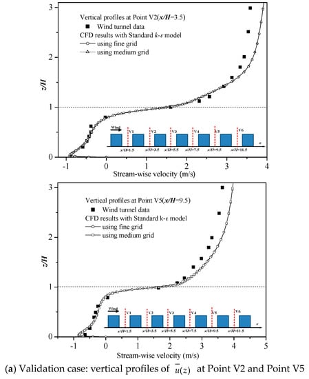
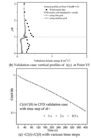
Figure 3.
CFD results and experimental data in the CFD validation case: (a,b) Vertical profiles of and at Point V2 and/or Point V5. (c) <C(t)>/C(0) with various time steps.
To further quantitatively evaluate the CFD models with the present grid arrangement and standard k-ε model, several statistical performance metrics are calculated, including the mean value, the standard deviation (named St dev. here), the fraction of predictions (here it is the CFD result) within a factor of two of observations (wind tunnel experiment data) named FAC2, the normalized mean error (NMSE), the fraction bias (FB), and the correlation coefficient (R). Results of at point V2 and V5 and at point V5 are shown in Table 2. According to the recommended reference criteria [52], for prediction, a good performing simulation model is supposed to meet the statistical metrics standards as below: FAC2 ≥ 0.5; NMSE ≤ 1.5; −0.3 ≤ FB ≤ 0.3. All the results satisfy the recommended criteria except the FB value of at point V5, which exceeds the upper limit, while its FAC2 just reaches the threshold. Furthermore, has a quite low R between wind tunnel data and CFD results. Results suggest a poorer quality of numerical prediction of than . As for , although it is overestimated as the FR is positive, the value of R is particularly high (0.93) at both V2 and V5, which implies a credible prediction of . Assessing models’ acceptance requires considering all relevant performance metrics rather than one specific index, so the CFD models are considered to have quite a satisfactory performance on the whole.
Table 2.
Statistical performance metrics in CFD validation case.
Finally, with this CFD setup, Figure 3c shows the effects of time steps on the decay history of spatial mean concentration (<C(t)>/C(0)). The decay rates for three time steps (dt = 0.5, 1, 2 s) are almost the same, confirming that the present time step (dt = 1 s) is good enough for ACH prediction.
3.2. Flow and Concentration Decay in an Example Case [5-5, 0°] (θ = 0°)
As an example to analyze the concentration decay history related to UCL ventilation, Figure 4 shows 3D streamline, normalized velocity (), normalized lateral velocity () in the plane of z = 0.05H, and normalized concentration (C(t)/C(0)) at a time of 10 s to 400 s in z = 0.5H in Case [5-5, 0°]. Here the velocity and lateral velocity are normalized by the freestream velocity at the same height of z = 0.05H (see Equation (1)), similar to the literature [17,18]. Then Figure 5 displays the concentration history (C(t)/C(0)) and the age of air (τp) at various points in z = 0.5H in Case [5-5, 0°]. In the main streets (Figure 4a), the flow is channeled toward downstream regions. In the secondary streets 3D vortices and helical flows exist in building wake regions. Across the lateral UCL boundary (at y = 135 m), there are lateral helical airflows leaving or re-entering UCL volume. Points with bigger concentration decay rates (K) experience better ventilation, a greater dilution rate, and smaller age of air (τp). Figure 4b and Figure 5a,b show that the ventilation in upstream regions is better than in downstream regions (Figure 5a), and that in the main streets it is better than in the secondary streets (Figure 5a); those (Point S1b–S4b) near the lateral UCL boundary are better than those (Point S1o–S4o) in urban center regions (Figure 5b). Figure 5b displays that K at Point S4b is near to Point S3b, and that at Point S4b near the UCL lateral boundaries it is much bigger than at Point S4o because there is a strong helical inflow across lateral boundaries, bringing in external air to help with pollutant dilution at Point S4b (Figure 4a). Similarly, in Figure 5c, the τp at Points M1b to M4b in the main streets is much smaller than Points S1a to S4a and Points S1o to S4o in the secondary streets. Moreover, air at Points S1b to S4b near lateral UCL boundaries is younger than Points S1o to S4o far from lateral UCL boundaries. More importantly, the τp at Points S4b, S4a, and S4o (89.5 to 249.4 s) verifies that the lateral inflow across UCL lateral boundaries significantly improves the ventilation at Point S4b.
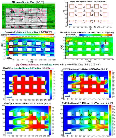
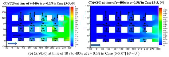
Figure 4.
In Case [5-5, 0°] (θ = 0°): (a) 3D streamline and normalized velocity in z = 0.05H; (b) C(t)/C(0) at time of 10 s to 400 s in plane of z = 0.5H.
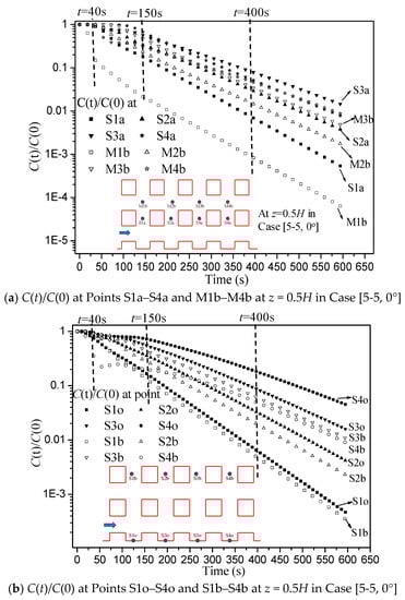
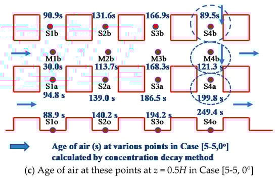
Figure 5.
C(t)/C(0) in Case [5-5, 0°]: (a) at Points S1a–S4a and M1b–M4b in z = 0.5H, (b) at Points S1o–S4o and S1b–S4b in z = 0.5H. (c) Age of air at these points.
There are qualitative differences between the decay curves in Figure 5a,b. Analyzing the behavior of the decay curves in Figure 5a, for example, after some time the decay rates at Points S1a and M1b are similar to each other. This is a manifestation that there is a coupling interaction between the two locations (more explanation can be found by comparing Figure 11.2 in [32]). However, in Figure 5b all curves exhibit different decay rates, which shows that is not feedback (no backflow against the wind direction) that connects the different locations (see also Chapter 11 in [32]).
3.3. Effect of Overall Urban Form and Ambient Wind Direction on UCL Ventilation
As an example, Figure 6 shows 3D streamline, normalized velocity, C(t)/C(0), and τp at various points in z = 0.5H in Case [5-5, 45°]. Here the velocity is normalized by the freestream velocity at the same height of z = 0.5H. Obviously wind brings clean air into an urban area downstream for pollutant dilution. There are recirculation regions with small wind speed (Figure 6a). Thus, the concentration decay rate (the age of air) is relatively small (large) in downstream regions and recirculation regions (Figure 6b,c).
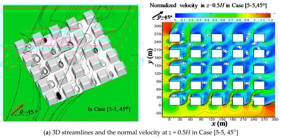
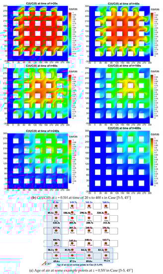
Figure 6.
In Case [5-5, 45°]: (a) 3D streamline and the normal velocity in z = 0.5H; (b) C(t)/C(0) in z = 0.5H at time of 20 s to 400 s; (c) age of air at some example points at z = 0.5H.
Then Figure 7a,b further displays the normalized velocity in Case [7-7, θ°] (square overall urban form) and Case [10-5, θ°] (rectangular overall urban form) with similar total UCL air volume. Obviously ambient wind directions significantly influence the flow pattern for both overall urban forms (Figure 7a,b). As θ = 0°, there are lateral flows across lateral UCL boundaries. With oblique winds, the flows enter UCL across two sides in upstream regions and leave across the other two toward downstream. The velocity is relatively small in recirculation regions and the presence of street crossings produces considerable momentum and scalar exchange between neighbor streets. In particular, Figure 7a confirms that, for square overall urban form, UCL models with θ = 45° experience more recirculation regions and quicker wind reduction than those with θ = 0°. It is consistent with the literature that building arrays with θ = 45° produce greater flow resistances and worse UCL ventilation performance than θ = 0° [2,7,23,58,59]. Such characteristics with θ = 45° produce adverse effects on its ventilation performance in contrast to θ = 0°.
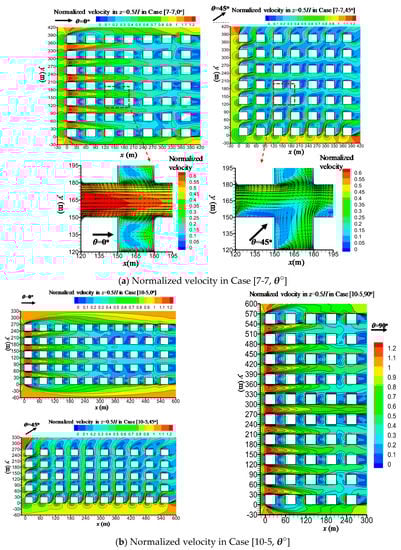
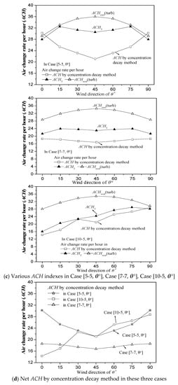
Figure 7.
Normalized velocity in (a) Case [7-7, θ°]; (b) case [10-5, θ°]; (c) Various ACH indexes in Case [5-5, θ°], Case [7-7, θ°], Case [10-5, θ°]; (d) Net ACH by concentration decay method in these three cases.
Then Figure 7c,d displays the net ACH by concentration decay method, ACHT and ACHturb in cases of Group I. Since Case [5-5, θ°] and Case [7-7, θ°] are of square overall urban form, the flows with θ = 0°, 15°, 30°, 45° are the same with those with θ = 90°, 75°, 60°, 45°. Obviously for Case [5-5, θ°] (Lx = Ly = 270 m) and Case [7-7, θ°] (Lx = Ly = 390 m), θ = 0° attains smaller ACHT and ACHturb but bigger net ACH than θ = 15°, 30°, 45°. Therefore, the parallel wind (θ = 0°) experiences the best overall UCL ventilation with the highest net ventilation efficiency. It can be explained that UCL models with non-parallel approaching wind (for example θ = 45° in Figure 7a) experience more recirculation regions and weaker wind due to the greater blockage induced by buildings, which can reduce the flow rates flushing through UCL space that never return or decrease the actual or net air change rate of the entire UCL space. Then for Case [10-5, θ°] with a rectangular overall urban form (Lx = 570 m, Ly = 270 m), as θ varies from 0° to 90°, ACHT rises from 16.1 h−1 to 29.0 h−1, ACHturb first increases from θ = 0° to θ = 45° then decreases to θ = 90°, and the net ACH rises from 14.3 h−1 to 28.7 h−1. Thus θ = 90° obtains the best overall UCL ventilation in Case [10-5, θ°], in which the approaching wind is parallel to the shorter urban size (Ly = 270 m). Finally, the net ACH by the concentration decay method are always much smaller than the sum of ACHturb and ACHT. This verifies that UCL ventilation efficiency is limited. As discussed in Section 2.4.2, the recirculation flows in UCL space and turbulent fluctuations across street roofs induce a significant fraction of fluid particles to return or revisit UCL space across UCL boundaries after they leave it. However, UCL ventilation mainly depends on the flow rates flushing UCL space and leaving it to never return. Thus only a fraction of ACHturb and ACHT contributes to UCL ventilation and the actual air change rate is limited due to the ventilation efficiency problems.
By comparing the net ACH in these three cases (Figure 7d), ACH in Case [5-5, θ°] (~21.1–30.2 h−1) are larger than those in Case [7-7, θ°] (~16.8–18.6 h−1) for all wind directions because Case [5-5, θ°] has smaller urban size and requires shorter time for the approaching wind to flow through and will be exchanged more times by the external air within one hour. Rectangular urban form (Case [10-5, θ°]) attains greater ACH (~21.1–28.7 h−1) than the square urban form (Case [7-7, θ°]~16.8–18.6 h−1) for most ambient wind directions except θ = 0° and 15° (~14.3 and 16.9 h−1). It can be explained by two example cases: for Case [10-5, 0°] there are 10 rows of buildings for the approaching wind to flush, much longer than Case [10-5, 90°], in which there are only five rows of buildings for wind to flow through.
3.4. Effect of Open Space Arrangements and Ambient Wind Direction
Open space arrangements have been regarded as one possible way to improve UCL ventilation. As shown in Table 1 (Group II), this subsection investigates 24 test cases with six kinds of open space arrangements under four wind directions (θ = 0°, 15°, 30°, 45°). Note that Oij represents the building of position i-j is removed for better ventilation. Figure 8a displays the 3D streamline in two example cases; Figure 8b further summarizes the net ACH by the concentration decay method in all 24 test cases.
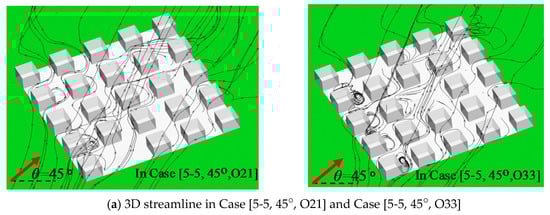
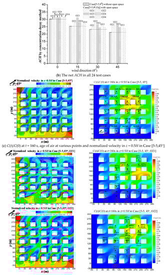
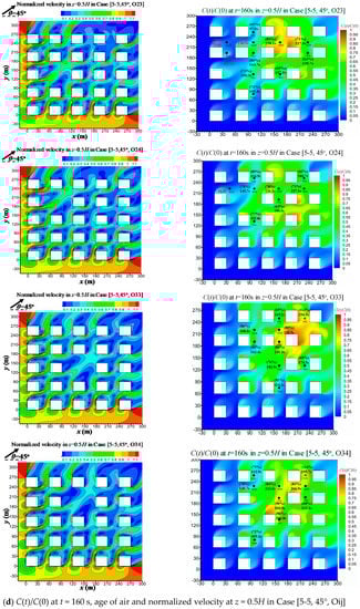
Figure 8.
(a) 3D streamline in Case [5-5, 45°, O21] and Case [5-5, 45°, O33]; (b) the net ACH in all 24 test cases. (c,d) C(t)/C(0) at t = 160 s, age of air at various points, and normalized velocity at z = 0.5H in Case [5-5, 45°] and Case [5-5, 45°, Oij].
Obviously, with oblique wind (θ = 15°, 30°, 45°) most open space arrangements improve UCL ventilation more than θ = 0° (see Figure 8b). The improvement of UCL ventilation is the best as θ = 45°. Thus θ = 45° is emphasized in the below analysis. Figure 8c,d shows C(t)/C(0) at t = 160 s, age of air (τp) at various points and normalized velocity in z = 0.5H in Case [5-5, 45°] and Case [5-5, 45°, Oij]. Because the open space arrangements act as a kind of ventilation corridor and reduce the total flow resistances induced by buildings, wind speed increases in regions near/surrounding open space and in its downstream regions; subsequently, the concentration decay processes speed up and the ventilation becomes better. The percentage data of τp in Figure 8d refer to the ratio between τp with open space (Case [5-5, 45°, Oij] in Figure 8d) and that without open space (Case [5-5, 45°] in Figure 8c). This percentage at some points can be from 12% to 65%, showing that τp significantly decreases in the regions near these points. Obviously, the effects of open space on flow pattern satisfy the variations of τp (Figure 8c,d) and overall ACH (Figure 8b).
4. Conclusions
As a novelty, this paper confirms the temporal decay profile of concentration in UCL models accords with the exponential decay law, and it is effective to introduce the concentration decay method into CFD simulations to predict the net air change rate (ACH) flushing UCL space and never returning. Street-scale (~100 m), medium-dense (λf = λp = 0.25, H/W = 1), urban-like geometries are studied under neutral atmospheric conditions. The standard k-ε model is first successfully evaluated by wind tunnel data. Then the flow pattern, the concentration decay rate and age of air (τp) at some points in UCL space, the net ACH are analyzed.
With a parallel approaching wind (θ = 0°), UCL models with larger urban sizes (Lx = Ly = 390 m) experience smaller ACH (~16.8–18.6 h−1) than smaller UCL models (Lx = Ly = 270 m, ACH~21.1–30.2 h−1). The urban age of air τp at points near upstream/lateral UCL boundaries is smaller (or the air is younger) than far from them. For the square overall urban form, the parallel wind attains greater net ACH than non-parallel wind (θ = 15°, 30°, 45°). For the rectangular overall urban form (Lx = 570 m, Ly = 270 m), ACH is greater than the square overall urban form (Lx = Ly = 390 m) under most wind directions (~21.1–28.7 h−1 as θ = 30° to 90°), and the ventilation is the best as the approaching wind is parallel to the shorter urban size (~28.7 h−1 as θ = 90°). With open space arrangements, the dilution capacity near/surrounding open space and in its downstream regions is enhanced; moreover, most open space arrangements are more effective at improving UCL ventilation under oblique wind directions (θ = 15°, 30°, 45°) than θ = 0°, and the best ventilation improvement by open space appears as θ = 45°.
Similar to the purging flow rate [2,23], ACH calculated by the concentration decay approach has been proven effective to evaluate the effects of urban morphologies on the overall UCL ventilation capacity induced by mean flows and turbulent diffusions, which seems to be a better ventilation index than ACH calculated by the volumetric flow rates integrating the normal mean velocity or fluctuation velocity across UCL boundaries. Turbulent diffusions across open street roofs have been proven to significantly contribute to UCL ventilation, but further investigations are still required to analyze the net ventilation efficiency by mean flows and turbulence.
Acknowledgments
This study was financially supported by the National Natural Science Foundation of China (grant No. 51478486) and the National Natural Science Foundation—Outstanding Youth Foundation (grant No. 41622502 ) as well as the Science and Technology Program of Guangzhou, China (grant No. 201607010066) and the Fundamental Research Funds for the Central Universities (No. 161gzd01).
Author Contributions
Qun Wang did the major CFD simulations. Yuanyuan Lin performed the CFD validation study. Mats Sandberg and Shi Yin contributed to the research discussion and writing the introduction. Jian Hang finished the manuscript and acts as the supervisor of the first author and corresponding author.
Conflicts of Interest
The authors declare no conflict of interest.
Nomenclature
| A | area of a surface (m2) |
| ACH | air change rate per hour by concentration decay method |
| ACHT | ACH calculated by QT for entire UCL volume |
| ACHturb | ACH calculated by Qroof(turb) for entire UCL volume |
| B, H, L, W | building width, building height, total length, street width |
| C, <C> | time-averaged pollutant concentration and its spatial mean value |
| , | turbulent eddy diffusivity of pollutant and momentum |
| λp | building area density (or plan area index) |
| λf | frontal area density (or frontal area index) |
| k, ε | turbulent kinetic energy and its dissipation rate |
| normal direction of street openings or canopy roofs | |
| Q | flow rate through street openings or street roofs |
| Qin, Qout | total inflow and outflow rate by mean flows across UCL boundaries |
| QT | total ventilation flow rate by mean flows |
| Qroof(turb) | effective flow rate across street roofs by turbulence |
| Sct | turbulent Schmidt number |
| fluctuation velocity on street roofs | |
| age of air (s) | |
| U0(z) | velocity profiles used at CFD domain inlet for ventilation cases |
| Uref | reference velocity at z = H at the domain inlet |
| , | velocity and coordinate components |
| velocity vector | |
| Vol | control volume |
| x, y, z | stream-wise, span-wise, vertical directions |
| , , | stream-wise, lateral, vertical velocity components |
| u′, v′, w′ | stream-wise, lateral, vertical velocity fluctuations |
References
- Oke, T.R. Boundary Layer Climates, 2nd ed.; Methuen Publishing: London, UK, 1987; p. 289. [Google Scholar]
- Bady, M.; Kato, S.; Huang, H. Towards the application of indoor ventilation efficiency indices to evaluate the air quality of urban areas. Build. Environ. 2008, 43, 1991–2004. [Google Scholar] [CrossRef]
- Hang, J.; Sandberg, M.; Li, Y.G. Age of air and air exchange efficiency in idealized city models. Build. Environ. 2009, 44, 1714–1723. [Google Scholar] [CrossRef]
- Buccolieri, R.; Sandberg, M.; Di Sabatino, S. City breathability and its link to pollutant concentration distribution within urban-like geometries. Atmos. Environ. 2010, 44, 1894–1903. [Google Scholar] [CrossRef]
- Hang, J.; Li, Y.G. Age of air and air exchange efficiency in high-rise urban areas. Atmos. Environ. 2011, 45, 5572–5585. [Google Scholar] [CrossRef]
- Ramponi, R.; Blocken, B.; Laura, B.; Janssen, W.D. CFD simulation of outdoor ventilation of generic urban configurations with different urban densities and equal and unequal street widths. Build. Environ. 2015, 92, 152–166. [Google Scholar] [CrossRef]
- Hang, J.; Luo, Z.W.; Sandberg, M.; Gong, J. Natural ventilation assessment in typical open and semi-open urban environments under various wind directions. Build. Environ. 2013, 70, 318–333. [Google Scholar] [CrossRef]
- Kim, J.J. Assessment of observation environment for surface wind in urban areas using a CFD model. Atmosphere 2015, 25, 449–459. (In Korean) [Google Scholar]
- Ashie, Y.; Kono, T. Urban-scale CFD analysis in support of a climate-sensitive design for the Tokyo Bay area. Int. J. Climatol. 2011, 31, 174–188. [Google Scholar] [CrossRef]
- Yang, X.; Li, Y.G. The impact of building density and building height heterogeneity on average urban albedo and street surface temperature. Build. Environ. 2015, 90, 146–156. [Google Scholar] [CrossRef]
- Hang, J.; Luo, Z.; Wang, X.; He, L.; Wang, B.; Zhu, W. The influence of street layouts and viaduct settings on daily CO exposure and intake fraction in idealized urban canyons. Environ. Pollut. 2017, 220, 72–86. [Google Scholar] [CrossRef] [PubMed]
- Luo, Z.; Li, Y.G.; Nazaroff, W.W. Intake fraction of nonreactive motor vehicle exhaust in Hong Kong. Atmos. Environ. 2010, 44, 1913–1918. [Google Scholar] [CrossRef]
- Ng, W.; Chau, C. A modeling investigation of the impact of street and building configurations on personal air pollutant exposure in isolated deep urban canyons. Sci. Total Environ. 2014, 468, 429–448. [Google Scholar] [CrossRef] [PubMed]
- Meroney, R.N.; Pavegeau, M.; Rafailidis, S.; Schatzmann, M. Study of line source characteristics for 2-D physical modelling of pollutant dispersion in street canyons. J. Wind Eng. Ind. Aerodyn. 1996, 62, 37–56. [Google Scholar] [CrossRef]
- Li, X.X.; Liu, C.H.; Leung, D.Y.C.; Lam, K.M. Recent progress in CFD modelling of wind field and pollutant transport in street canyons. Atmos. Environ. 2006, 40, 5640–5658. [Google Scholar] [CrossRef]
- Li, X.X.; Liu, C.H.; Leung, D.Y.C. Numerical investigation of pollutant transport characteristics inside deep urban street canyons. Atmos. Environ. 2009, 43, 2410–2418. [Google Scholar] [CrossRef]
- Zhang, Y.W.; Gu, Z.; Lee, S.C.; Fu, T.M.; Ho, K.F. Numerical simulation and in situ investigation of fine particle dispersion in an actual deep street canyon in Hong Kong. Indoor Built Environ. 2011, 20, 206–216. [Google Scholar] [CrossRef]
- Lin, L.; Hang, J.; Wang, X.X.; Wang, X.M.; Fan, S.J.; Fan, Q.; Liu, Y.H. Integrated effects of street layouts and wall heating on vehicular pollutant dispersion and their reentry into downstream canyons. Aerosol Air Qual. Res. 2016, 16, 3142–3163. [Google Scholar] [CrossRef]
- Dong, J.L.; Tan, Z.J.; Xiao, X.M.; Tu, J.Y. Seasonal changing effect on airflow and pollutant dispersion characteristics in urban street canyons. Atmosphere 2017, 8, 43. [Google Scholar] [CrossRef]
- Gu, Z.; Zhang, Y.; Cheng, Y.; Lee, S.C. Effect of uneven building layout on air flow and pollutant dispersion in non-uniform street canyons. Build. Environ. 2011, 46, 2657–2665. [Google Scholar] [CrossRef]
- Hang, J.; Li, Y.; Sandberg, M.; Buccolieri, R.; Di Sabatino, S. The influence of building height variability on pollutant dispersion and pedestrian ventilation in idealized high-rise urban areas. Build. Environ. 2012, 56, 346–360. [Google Scholar] [CrossRef]
- Panagiotou, I.; Neophytou, M.K.A.; Hamlyn, D.; Britter, R.E. City breathability as quantified by the exchange velocity and its spatial variation in real inhomogeneous urban geometries: An example from central London urban area. Sci. Total Environ. 2013, 442, 466–477. [Google Scholar] [CrossRef] [PubMed]
- Lin, M.; Hang, J.; Li, Y.G.; Luo, Z.W.; Sandberg, M. Quantitative ventilation assessments of idealized urban canopy layers with various urban layouts and the same building packing density. Build. Environ. 2014, 79, 152–167. [Google Scholar] [CrossRef]
- Lee, D.; Kim, J.J. A study on the characteristics of flow and reactive pollutants’ dispersion in step-up street canyons using a CFD model. Atmosphere 2015, 25, 473–482. (In Korean) [Google Scholar] [CrossRef]
- Chen, L.; Hang, J.; Sandberg, M.; Claesson, L.; Di Sabatino, S.; Wigo, H. The impacts of building height variations and building packing densities on flow adjustment and city breathability in idealized urban models. Build. Environ. 2017, 118, 344–361. [Google Scholar] [CrossRef]
- Li, X.X.; Britter, R.E.; Norford, L.K. Transport processes in and above two-dimensional urban street canyons under different stratification conditions: results from numerical simulation. Environ. Fluid Mech. 2015, 15, 399–417. [Google Scholar] [CrossRef]
- Nazarian, N.; Kleissl, J. Realistic solar heating in urban areas: Air exchange and street-canyon ventilation. Build. Environ. 2016, 95, 75–93. [Google Scholar] [CrossRef]
- Cui, P.Y.; Li, Z.; Tao, W.Q. Wind-tunnel measurements for thermal effects on the air flow and pollutant dispersion through different scale urban areas. Build. Environ. 2016, 97, 137–151. [Google Scholar] [CrossRef]
- Wang, X.X.; Li, Y.G. Predicting urban heat island circulation using CFD. Build. Environ. 2016, 99, 82–97. [Google Scholar] [CrossRef]
- Fan, Y.F.; Hunt, J.C.R.; Li, Y.G. Buoyancy and turbulence-driven atmospheric circulation over urban areas. J. Environ. Sci. 2017. [Google Scholar] [CrossRef]
- Hang, J.; Wang, Q.; Chen, X.Y.; Sandberg, M.; Zhu, W.; Buccolieri, R.; Di Sabatino, S. City breathability in medium density urban-like geometries evaluated through the pollutant transport rate and the net escape velocity. Build. Environ. 2015, 94, 166–182. [Google Scholar] [CrossRef]
- Etheridge, D.; Sandberg, M. Building Ventilation: Theory and Measurement; John Wiley & Sons: New York, NY, USA, 1996; pp. 573–633. [Google Scholar]
- Lim, E.S.; Ito, K.; Sandberg, M. New ventilation index for evaluating imperfect mixing conditions—Analysis of Net Escape Velocity based on RANS approach. Build. Environ. 2013, 61, 45–56. [Google Scholar] [CrossRef]
- Li, J.Q.; Ward, I.C. Developing computational fluid dynamics conditions for urban natural ventilation study. In Proceedings of the Building Simulation, Beijing, China, 3–6 September 2007. [Google Scholar]
- Zaki, S.A.; Hagishima, A.; Tanimoto, J. Experimental study of wind-induced ventilation in urban building of cube arrays with various layouts. J. Wind Eng. Ind. Aerodyn. 2012, 103, 31–40. [Google Scholar] [CrossRef]
- Padilla-Marcos, M.Á.; Meiss, A.; Feijó-Muñoz, J. Proposal for a simplified CFD procedure for obtaining patterns of the age of air in outdoor spaces for the natural ventilation of buildings. Energies 2017, 10, 1252. [Google Scholar] [CrossRef]
- Li, X.X.; Liu, C.H.; Leung, D.Y.C. Development of a k-ε model for the determination of air exchange rates for street canyons. Atmos. Environ. 2005, 39, 7285–7296. [Google Scholar] [CrossRef]
- Liu, C.H.; Leung, D.Y.C.; Barth, M.C. On the prediction of air and pollutant exchange rates in street canyons of different aspect ratio using large-eddy simulation. Atmos. Environ. 2005, 39, 1567–1574. [Google Scholar] [CrossRef]
- Moonen, P.; Dorer, D.; Carmeliet, J. Evaluation of the ventilation potential of courtyards and urban street canyons using RANS and LES. J. Wind Eng. Ind. Aerodyn. 2011, 99, 414–423. [Google Scholar] [CrossRef]
- Hang, J.; Sandberg, M.; Li, Y. Effect of urban morphology on wind condition in idealized city models. Atmos. Environ. 2009, 43, 869–878. [Google Scholar] [CrossRef]
- Hang, J.; Li, Y.G. Ventilation strategy and air change rates in idealized high-rise compact urban areas. Build. Environ. 2010, 45, 2754–2767. [Google Scholar] [CrossRef]
- Liu, J.; Luo, Z.; Zhao, J.; Shui, T. Ventilation in a street canyon under diurnal heating conditions. Int. J. Vent. 2012, 11, 141–154. [Google Scholar] [CrossRef]
- Yang, L.; Li, Y.G. City ventilation of Hong Kong at no-wind conditions. Atmos. Environ. 2009, 43, 3111–3121. [Google Scholar] [CrossRef]
- Yang, L.; Li, Y.G. Thermal conditions and ventilation in an ideal city model of Hong Kong. Energy Build. 2011, 43, 1139–1148. [Google Scholar] [CrossRef]
- Gao, N.P.; Niu, J.L.; Perino, M.; Heiselberg, P. The airborne transmission of infection between flats in high-rise residential buildings: Tracer gas simulation. Build. Environ. 2008, 43, 1805–1817. [Google Scholar] [CrossRef]
- Hooff, V.T.; Blocken, B. CFD evaluation of natural ventilation of indoor environments by the concentration decay method: CO2 gas dispersion from a semi-enclosed stadium. Build. Environ. 2013, 61, 1–17. [Google Scholar] [CrossRef]
- Fernando, H.J.S.; Zajic, D.; Di Sabatino, S.; Dimitrova, R.; Hedquist, B.; Dallman, A. Flow, turbulence, and pollutant dispersion in urban atmospheres. Phys. Fluids 2010, 22, 051301. [Google Scholar] [CrossRef]
- Di Sabatino, S.; Buccolieri, R.; Salizzoni, P. Recent advancements in numerical modelling of flow and dispersion in urban areas: a short review. Int. J. Environ. Pollut. 2013, 52, 172–191. [Google Scholar] [CrossRef]
- Blocken, B. Computational fluid dynamics for urban physics: Importance, scales, possibilities, limitations and ten tips and tricks towards accurate and reliable simulations. Build. Environ. 2015, 91, 219–245. [Google Scholar] [CrossRef]
- Brown, M.J.; Lawson, R.E.; DeCroix, D.S.; Lee, R.L. Comparison of Centerline Velocity Measurements Obtained Around 2D and 3D Buildings Arrays in a Wind Tunnel; Report LA-UR-01–4138; Los Alamos National Laboratory: Los Alamos, NM, USA, 2001; p. 7.
- Lien, F.S.; Yee, E. Numerical modelling of the turbulent flow developing within and over a 3-D building array, part I: A high-resolution Reynolds-averaged Navier-Stokes approach. Bound. Layer Meteorol. 2004, 112, 427–466. [Google Scholar] [CrossRef]
- Santiago, J.L.; Martilli, A.; Martin, F. CFD simulation of airflow over a regular array of cubes Part I: Three-dimensional simulation of the flow and validation with wind-tunnel measurements. Bound. Layer Meteorol. 2007, 122, 609–634. [Google Scholar] [CrossRef]
- Hang, J.; Li, Y.G. Wind conditions in idealized building clusters: Macroscopic simulations by a porous turbulence model. Bound. Layer Meteorol. 2010, 136, 129–159. [Google Scholar] [CrossRef]
- Tominaga, Y.; Mochida, A.; Yoshie, R.; Kataoka, H.; Nozu, T.; Yoshikawa, M.; Shirasawa, T. AIJ guidelines for practical applications of CFD to pedestrian wind environment around buildings. J. Wind Eng. Ind. Aerodyn. 2008, 96, 1749–1761. [Google Scholar] [CrossRef]
- Franke, J.; Hellsten, A.; Schlunzen, H.; Carissimo, B. The COST732 Best Practice Guideline for CFD simulation of flows in the urban environment: A summary. Inter. J. Environ. Pollut. 2011, 44, 419–427. [Google Scholar] [CrossRef]
- FLUENT V6.3. User’s Manual. Available online: http://www.fluent.com (accessed on 20 August 2017).
- Blocken, B.; Stathopoulos, T.; Carmeliet, J. CFD simulation of the atmospheric boundary layer: Wall function problems. Atmos. Environ. 2007, 41, 238–252. [Google Scholar] [CrossRef]
- Kim, J.J.; Baik, J.J. A numerical study of the effects of ambient wind direction on flow and dispersion in urban street canyons using the RNG k-ε turbulence model. Atmos. Environ. 2004, 38, 3039–3048. [Google Scholar] [CrossRef]
- Kanda, M. Large-eddy simulations on the effects of surface geometry of building arrays on turbulent organized structures. Bound. Layer Meteorol. 2006, 18, 151–168. [Google Scholar] [CrossRef]
© 2017 by the authors. Licensee MDPI, Basel, Switzerland. This article is an open access article distributed under the terms and conditions of the Creative Commons Attribution (CC BY) license (http://creativecommons.org/licenses/by/4.0/).