Decadal Spatial-Temporal Variations in the Spatial Pattern of Anomalies of Extreme Precipitation Thresholds (Case Study: Northwest Iran)

Abstract

This study focused on decadalvariations of extreme precipitation thresholds within a 50-year period (1961–2010) for 250 stations of Iran’s northwest. The 99th percentile was used as the threshold of extreme precipitation. In order to analyze threshold cycles and spatial autocorrelation pattern dominating extreme precipitation thresholds, spectral analysis and Gi (known as HOTSPOT) were used respectively. The results revealed that the highest threshold of extreme precipitation occurred along the Ghoosheh Dagh mountain range. Additionally, in all the five studied decades, the highest positive anomalies were observed in the same region (i.e., the Ghoosheh Dagh). The findings also showed that the intensity of positive spatial autocorrelation pattern of extreme precipitation thresholds experienced a declining trend in recent decades. At the same time, extreme precipitation weighted mean center indicated that they followed an ordered pattern during the studied period. The results of harmonic analysis demonstrated that, in all decades, short-term (2–4 years) and mid-term (4–8 years) cycles of extreme precipitation thresholds were dominated. However, especially the southwest of the studied area, the return period of extreme precipitation thresholds was as long as the studied period, a phenomenon that indicates the existence of a trend in extreme precipitation thresholds of these regions.

1. Introduction

Changes in extreme weather and climate events have significant impacts and are among the most serious challenges to society in coping with a changing climate [1]. Changes in the frequency and intensity of climatic events are an indicator of climate change [2]. Considerable attention is being paid to the spatial-temporal pattern of precipitation. In fact, this climate element is not stable at all and has a lot of spatial variations. Understanding precipitation variability in the arid, rugged landscapes of Iran requires studying the climatology and spatial patterns of daily precipitation [3]. On the other hand, because of the diversity of precipitation sources in different parts of Iran, the amount and time of precipitation varies widely from one place to another [4,5]. This spatial and temporal variation indicates that average precipitation is not a good index for studying precipitation pattern [6] since it does not encompass all climate features [7]. It is likely that a change in climate aspects occurs without any noticeable variation in precipitation average [8,9,10]. For example, changes in the extreme weather events may have important consequences and are thus regarded as an essential issue in climate change [10]. There is growing evidence at global, regional, and local scales that intra-annual precipitation regimes have already become more extreme [11,12]. For example, global precipitation records show an average increase of only 9 millimeters (mm) of precipitation over land areas (excluding Antarctica) during the 20th century [13]. Regionally, however, these records show an increased frequency of wet days in portions of North America, Europe, and Southern Africa; an increased frequency and duration of dry periods in European-African, Australian, Mediterranean, and Asian monsoon regions; and an increased proportion of total precipitation originating from the largest precipitation events in several regions [13,14,15,16]. Therefore, numerous studies have focused on extreme precipitation (which is regarded as an extreme weather event). Alexander et al. (2006) studied global changes in extreme temperature and precipitation [17]. Extreme precipitation has also been investigated in Sicily [18], India [19], Sao Paulo [20], south of Poland and central-eastern Germany [21], and Switzerland [22]. In a study conducted in England, Hand et al. (2004) showed that frontal precipitation occurs when relative humidity is over 80% and trough passes within 200 km from the south or east of the location where extreme precipitation happens. Extreme convectional precipitation occurs in June, July, and August. Finally, extreme orographic precipitation occurs in December, January, and February [23]. In another study, Unkasevic (2000) studied the extreme precipitation occurrence in Serbia and Montenegro. Their results displayed that two extreme precipitation occurred because a cyclonic and anticyclonic system was formed over Serbia for several days [24]. Seibert et al. conducted cluster analysis to come up with the synoptic patterns of extreme precipitation in Austria [25]. Matlik and Piia (2008) also investigated climate models generating extreme rains in Estonia. In order to find out how extreme precipitation occurs, they studied cyclone, front paths, and troughs. They found that extreme precipitation mainly occurs due to troughs and fronts. They concluded that south cyclones which originate from the Black Sea and the Mediterranean Sea play the most significant role in the occurrence of extreme precipitation in Estonia [26].

A number of similar studies have been conducted in Iran. Soltani et al. (2016) and Rahimzadeh et al. (2009), for example, investigated decadal variations of extreme precipitation in Iran, they showed that there are significant trends in extreme precipitation events [27,28]. Further, Rousta et al. (2016 and 2017) and Zolfaghari et al. (2009) concentrated on the ratio of maximum daily precipitation to annual precipitation and they concluded that the southward movement of Polar Vortex is considered as those important factors to produce extreme precipitation events over Iran [29,30,31]. Finally, Soltani et al. (2014) and Asakereh (2012) investigated extreme precipitation in Kerman and Zanjan provinces [8,32], while Soltani et al. (2013) investigated the long-term precipitation in Gorgan province [33] and Alijani (2011) focused on extreme values of climate elements and they are showed that the heavy rains are increased all over the country [34].

As mentioned above, changes in climatic extremes of Iran and the world are of paramount importance. Therefore, the present study aimed at investigating the anomalies, spatial pattern, and the cyclones that dominate extreme precipitation thresholds in the northwest of Iran. The study focused on decadalvariations within a 50-year period (1961–2010).

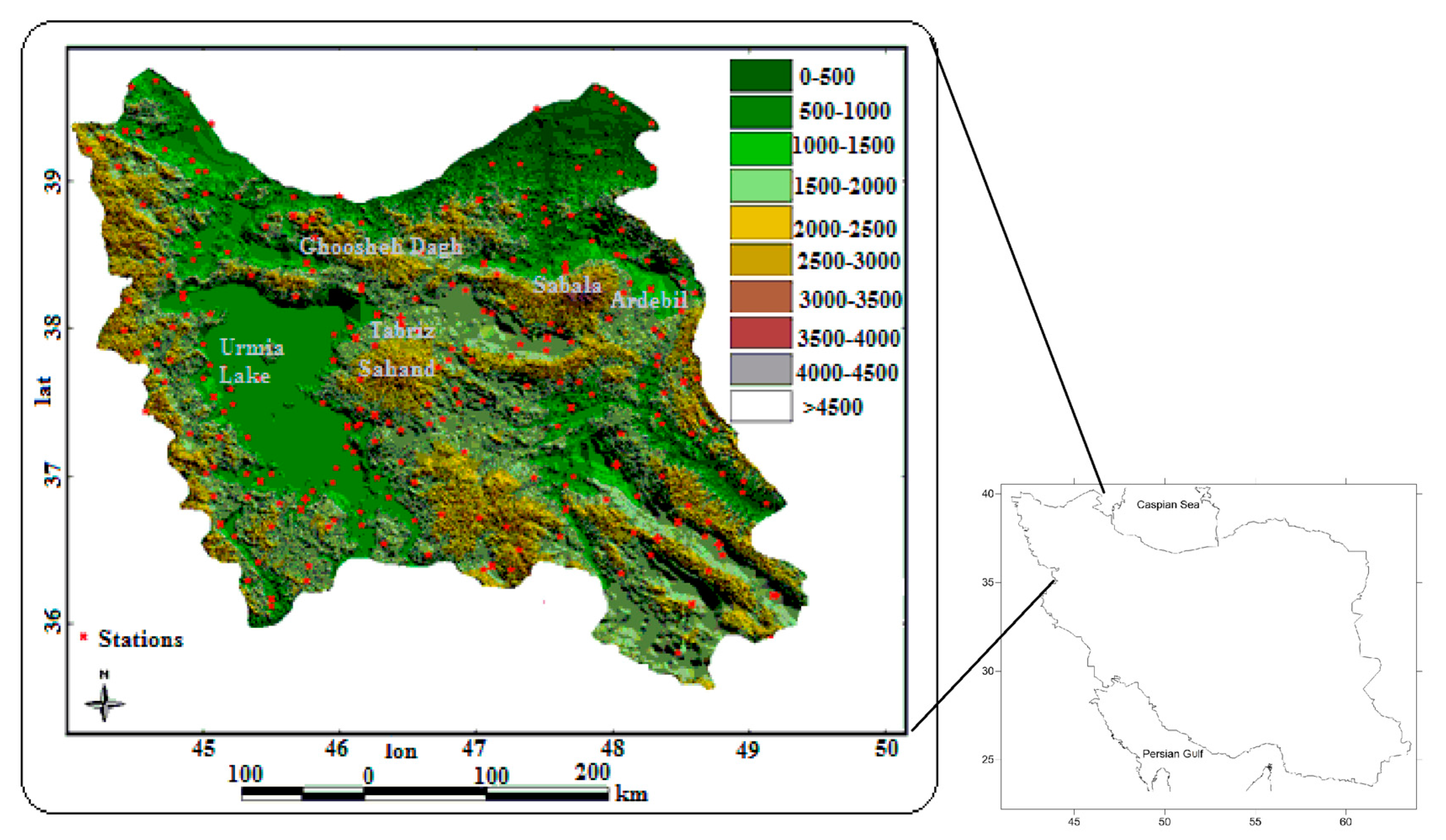
2. Materials and Method

In order to analyze the spatial pattern, anomalies, and cycles of extreme precipitation threshold in the northwest of Iran (including the provinces of Ardabil, East Azerbaijan, West Azerbaijan, and Zanjan), precipitation height data were collected from 250 climatologic and synoptic stations and rain gauges of Iran’s Meteorological Organization for a 50-year period (1960–2010). Figure 1 illustrates the distribution of the stations and the heights of the studied regions.

Not all the used stations had full record of the necessary data from the beginning of the studied period. Therefore, Kriging interpolation was used to compensate for the missing data. That is, a precipitation map was developed for each day of the period (which ranged from the first day of 1961 to the last day of 2010). Surfer was used for constructing the maps. This process led to the development of 18,266 daily maps, with each one containing 1266 cells inside the studied region. In the next step, based on the daily maps, an 18,266 × 1266 matrix was constructed. In order to study extreme precipitation, the 99th percentile of daily precipitation was considered as the threshold. Spatial distribution of precipitation in the northwest of Iran is different in each year and every month [8,35,36,37]. Therefore, in this paper, in order to study the exact thresholds of extreme precipitation in northwest of Iran, extreme daily precipitation threshold is calculated for each month during the study period by using following formula:

$$P_{99}=\frac{99\times \mathrm{n}}{100}\text{ For Odd data}$$

(1)

$$P_{99}=\frac{99\times \mathrm{n}}{100}+\frac{1}{2}\text{ For Even data}$$

(2)

As a result, a 600 × 1264 database was constructed for extreme precipitation thresholds. With the aim of developing a better understanding of precipitation threshold variations, this matrix was divided into five decades (1960–1970, 1971–1980, 1981–1990, 1991–2000, and 2001–2010). Because almost recent researches into Iran’s precipitation show that extreme precipitation have a return periods about 10 to 13 years [36,37,38,39,40,41]. Therefore, according to these research, 10-year periods were also selected in this study. In order to gain an overall view of the spatial pattern of extreme precipitation threshold variations in the northwest of Iran, mean, anomaly, and weighted mean center maps of extreme precipitation thresholds were designed. Subsequently, in order to find out the dominant pattern in these thresholds, Hot Spot Analysis, Getis-Ord Gi (which is one of the common indices for identifying spatial autocorrelation of observations and their spatial pattern) was exploited. This analytical procedure helps researchers find out if the studied elements follow a cluster or dispersed pattern. Using Z-score as a yardstick, this analytical procedure shows the areas in which clusters are formed. In this procedure, every phenomenon is interpreted in the light of its neighboring ones. High values of a phenomenon may be indicative of an interesting or significant issue; however, it may not represent a statistically hot spot. Both the particular phenomenon and its neighboring ones should have high values to be regarded as a hot spot. Getis-Ord Gi is calculated through the following formula [42]:

$$G_i^{*}=\frac{{{\displaystyle \sum }}_{j=1}^n{w}_{i.j}{x}_j-\overline{X} {{\displaystyle \sum }}_{j=1}^n{w}_{i.j}}{S \sqrt{\frac{n {{\displaystyle \sum }}_{j=1}^n{w}_{i,j}^2-\left({{\displaystyle \sum }}_{j=1}^n{w}_{i.j}\right)}{n-1}}}$$

(3)

where $X_j$ is the amount of phenomenon j, $w_{i.j}$ is the spatial weight between phenomena i and j, and n indicates the number of entire phenomena:

$$S=\sqrt{\frac{{\sum }_{j=1}^n{x}_i^2}{n}-{(\overline{X})}^2},\overline{X}=\frac{{\sum }_{j=1}^n{x}_i}{n}$$

(4)

In order to have a more accurate understanding of decadal variations of extreme precipitation, spectral analysis was conducted to investigate precipitation cycles in each period. The distribution of variance along all wavelengths of the time series is known as spectral analysis. In fact, the harmonic analysis technique entails analyzing the variance of a time series. In spectral analysis, time series are first converted to frequency functions (in the form of periodic functions with amplitude and frequency). In such functions, frequency indicates the time scale (cycles within a time unit) and amplitude represents variance in this time scale. Therefore, in this technique, each of the waves is extracted and their contribution to the total variance is assessed. Then, after determining the variance, each of the waves is studied to see if they are statistically significant. In order to convert the time series to frequency and calculate the harmonics, first, two parameters should be calculated:

$$a_i=\frac{2}{n}{{\displaystyle \sum }}_{t=1}^n{x}_{t}cos\left(\frac{2\pi q}{n}t\right) q=1,2, \dots ,\frac{n}{2}$$

(5)

$$b_i=\frac{2}{n}{{\displaystyle \sum }}_{t=1}^n{x}_{t}sin\left(\frac{2\pi q}{n}t\right) q=1,2, \dots ,n$$

(6)

where q is the number of harmonics. For even series, there will be $q=\frac{n}{2}$ harmonics, whereas for odd series, there will be $q=\frac{\left(n-1\right)}{2}$. harmonics.

The variance of each frequency (wave) is calculated through the following formula:

$$I\left(f_i\right)=\frac{n}{2}\left(a_i^2+ b_i^2\right)$$

(7)

In order to conduct the significance test, first the following three steps must be taken:

A: calculating the spectral mean ($\overline{S}$), B: calculating the first order autocorrelation for the observations of time series of data ($r_1$), C: calculating the spectrum for a random series with the mean of ($\overline{S}$) and the first order autocorrelation of ($r_1$) by the use of the following formula [43]:

$$\mathrm{I}\left({\mathit{F}}_{\mathit{i}}\right)=\overline{\mathrm{S}}\left[\frac{1-{\mathit{r}}_1^2}{1+{\mathit{r}}_1^2-2{\mathit{r}}_1\cos \left(\frac{\mathsf{\pi }\times \mathrm{i}}{\mathrm{q}}\right)}\right]\mathit{i}=1,2,\dots ,\mathit{q}$$

(8)

where $\mathrm{I}\left({\mathrm{F}}_{\mathrm{i}}\right)$ is the variance of the harmonics which belong to the random series. In order to conduct the significance test, first a confidence interval is determined (typically 95%). Each of the spectra (frequencies) of the time series that are out of this interval is regarded as significant cycles. ${\chi }^2$ is used in order to test the significance. The degree of freedom of the test is calculated through the following formula:

$$df= \frac{2n- \frac{q}{2}}{q}$$

(9)

Considering this degree of freedom and the confidence interval (95%), the values of ${\chi }^2$ table are used to calculate the significance level through the following formula:

$$\mathrm{sig}\mathit{I}\left(\mathit{F}\right)=\frac{{\mathit{x}}^2}{\mathrm{df}}\times \mathit{I}\left(\mathit{f}\right)$$

(10)

The cycles in which the amount of variance is $I\left(f\right)>\widehat{I}\left(f\right)$ are significant.

Weighted Mean Center is one of the ways to examine the distribution of phenomena and its variabilities over time. A weighted mean center provides a description of the central tendency when points or locations have different frequencies or occurrences of the phenomenon studied. Given points representing the locations of endangered plant species, it makes more sense to calculate their mean center by using the sizes of plant communities at each location as weight of the points. The weighted mean center of a distribution can be found by multiplying the x and y coordinates of each point by the weights assigned to them. The mean of the weighted x coordinates and the mean of the weighted y coordinates define the position of the weighted mean center. The equation for the weighted mean center is: [44].

$${\overline{\mathrm{X}}}_{wm\mathrm{c}};{\overline{\mathrm{Y}}}_{\mathrm{wmc}}=(\frac{{{\displaystyle \sum }}_{\mathrm{i}=1}^{\mathrm{n}}{\mathit{w}}_{\mathit{i}}{\mathrm{X}}_{\mathrm{i}}}{{{\displaystyle \sum }}_{\mathrm{i}=1}^{\mathrm{n}}{\mathit{w}}_{\mathit{i}}}; \frac{{{\displaystyle \sum }}_{\mathrm{i}=1}^{\mathrm{n}}{\mathit{w}}_{\mathit{i}}{\mathrm{X}}_{\mathrm{i}}}{{{\displaystyle \sum }}_{\mathrm{i}=1}^{\mathrm{n}}{\mathit{w}}_{\mathit{i}}})$$

(11)

where ${\overline{\mathrm{X}}}_{wm\mathrm{c}}; {\overline{\mathrm{Y}}}_{\mathrm{wmc}}$ defines the weighted mean center, and w_i is the weight at point p_i (that in current study p_i is the extreme precipitation thresholds).

MATLAB was used to conduct all the above-mentioned calculations. Furthermore, Arc GIS was utilized to run spatial analysis.

3. Results and Discussion

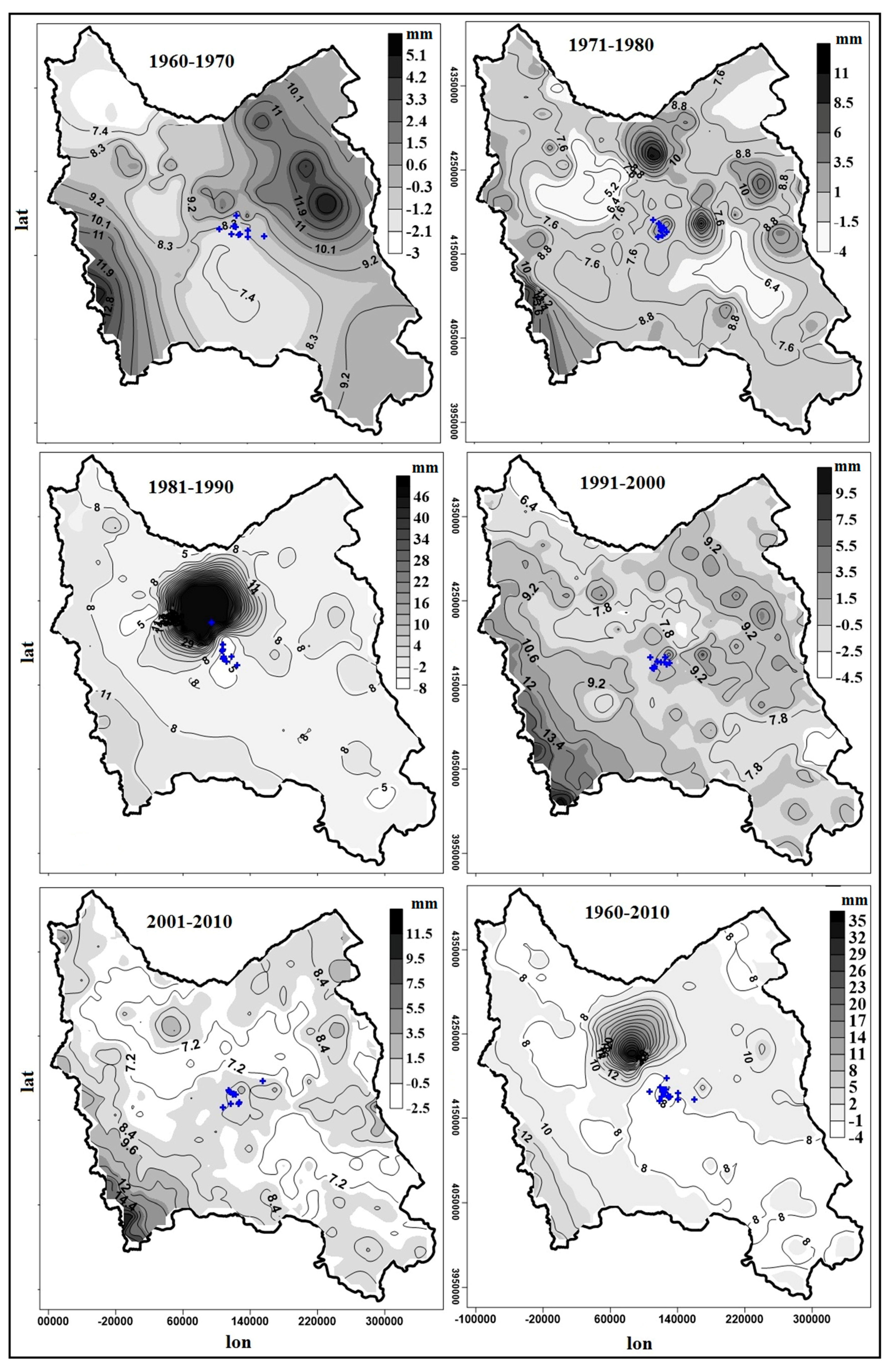
3.1. General Features of Extreme Precipitation

Table 1. Descriptive statistics of extreme precipitation thresholds in the northwest of Iran during different periods.

Index	1961–1970	1971–1980	1981–1990	1991–2000	2001–2010	1961–2010
mean	9.2	8.4	11.2	9.1	8.1	9.2
median	8.9	7.9	7.5	8.7	8.0	8.2
mode	5.8	6.3	7.3	6.1	7.0	4.7
var	8.9	8.1	2363.2	7.7	10.7	480.8
std	3.0	2.8	48.6	2.8	3.3	21.9
cv	32.3	33.9	433.8	30.4	40.2	237.8
Skewness	1.1	2.8	20.2	1.5	0.6	44.4
kurtosis	6.0	25.0	491.9	7.0	7.0	239.1
max	29.5	51.0	165.5	28.5	33.7	165.5
Q1	7.2	6.6	6.1	7.3	6.8	6.8
Q2	8.9	7.9	7.5	8.7	8.0	8.2
Q3	10.9	9.6	9.4	10.4	9.6	10.1

contains some of the features of extreme precipitation thresholds during various periods. The maximum mean score of extreme precipitation threshold (11.2 mm) belongs to the third period (1981–1990), while the minimum mean score was recorded in the fifth one (2001–2010). In the five studied decades, there is a considerable difference between mean, mode, and median, a phenomenon that indicates lack of normal distribution in the extreme precipitation thresholds of the northwest of Iran. In other words, the huge difference between mode, median, and mean shows that extreme precipitation thresholds of the northwest of Iran have experienced a lot of ups and downs during the five periods and have not followed a normal distribution. More specifically, the low quartile range supports the idea that extreme precipitation thresholds have had a lot of oscillations during various periods.

The highest coefficient of spatial variation of extreme precipitation threshold (433.8%) was registered in the third period, while the lowest coefficient of variation (30.39%) was recorded in the fourth decade. This indicates that extreme precipitation thresholds in the northwest of Iran have experienced both spatial and daily variation during the third period. In other words, the high coefficient of variation indicates daily instability and oscillations of extreme precipitation thresholds during this decade. Skewness was positive for all the periods, which means that extreme precipitation thresholds were positively skewed during all the five studied periods. Positive skewness means that the values have tendency to values greater than average and inverse for negative skewness. And for the central markers when they are closed, its means low variability and inverse when it is sporadic [45]. In other words, for each decade, the area with below average precipitation thresholds was larger than the one with precipitation threshold above the mean. The highest recorded extreme precipitation threshold (165.5 mm) belonged to the third period. In order to gain an overall view of the spatial pattern of extreme precipitation threshold, the spatial distributions of mean, anomaly, and weighted mean center of these thresholds are illustrated in Figure 2. The presented maps in this figure show the difference between annual average maps for each period and extreme precipitation threshold average for the same period. Areas with positive anomaly are indicated with dark color, while areas with negative anomaly are illustrated with light color. Positive anomalies indicate an increase in extreme precipitation thresholds in a decade (compared to the entire studied period), whereas negative anomalies demonstrate a decline in extreme precipitation thresholds.

In these figures, contours show mean spatial distribution, different colors indicate the range of anomalies, and blue signs illustrate weighted mean centers of extreme precipitation thresholds in the northwest of Iran. The mean spatial distribution displays that, during the five periods, the majority of the northwest area had an average threshold of 6 to 8 mm. However, in the first period (1961–1970), the maximum extreme precipitation thresholds concentrated along Mount Sabalan and some parts of the southwest of the studied area. Therefore, highlands, especially Mount Sahand and Sabalan, play a significant role in the occurrence of extreme precipitation thresholds in this region. Some researchers believe that the three patterns of Saudi low pressure-Siberian high pressure, Siberian high pressure-North East Africa/Saudi low pressure, and West Russia high pressure/Iraq-Saudi low pressure are influential in extreme and pervasive precipitation of Iran [46]. The highest amount of precipitation occurred in the region where northwest winds enter Iran and face windward slopes of mountains. Nevertheless, mountains are not the only factor contributing to precipitation increase. Some other parameters, like the region from which Mediterranean cyclones and west winds enter Iran, are influential as well [47]. In this period (1961–1970), nonetheless, only 4.7% of the area had a precipitation mean above 12 mm. The second period is almost similar to the first one. The only difference is that, during the first period, the majority of the studied area had a precipitation threshold of 8 to 10 mm, while, in the second period, a precipitation threshold of 6 to 10 mm was recorded for the largest part of the region. The highest thresholds were recorded in the third decade (illustrated by a black spot in Figure 2). However, in this period, the largest area of northwest Iran had a precipitation average of 6 to 8 mm. Only 2.3% of the area which is located along the Ghoosheh Dagh mountain range had a threshold of more than 14 mm. Arasbaran, which is located in the northern part of this region, might also be effective in its high threshold. During the fourth and fifth periods, extreme precipitation threshold averages experienced a significant decline; however, the spatial distribution of thresholds was more homogenous compared to the previous periods. For example, the threshold coefficient of variation was extremely high during the third period. In all the periods, the spatial distribution of anomalies of extreme precipitation thresholds follows the spatial distribution pattern of heights. Thus, in all the five studied periods, highlands of northwest Iran had positive anomalies, while lowlands experienced negative anomalies. In the first decade (1961–1970), the range of extreme precipitation threshold anomalies was smaller. The highest range (from −8 mm to 45 mm) belonged to the third period. The highest positive anomaly is illustrated in the form of a black spot along the Ghoosheh Dagh and Arasbaran. In this period, the largest area of the studied region (over 80%) had negative anomaly.

In the fourth decade, the intensity of negative anomalies reduced, while that of positive anomalies went up. During this time, around 37% of the studied region (mainly including southwest area of the region) had positive anomaly. Negative anomalies considerably increased during the fifth decade. Although the Ghoosheh Dagh heights had positive anomaly during the previous decades, they experienced negative anomaly during this period. The highest positive anomaly is illustrated in the form of a black spot in the southwest of the studied region. In total, the highest area of the studied region had negative anomaly.

The mean and weighted mean center of extreme precipitation threshold were designed for the five decades in order to gain a better understanding of spatial behavior and regularity of extreme precipitation threshold in the northwest of Iran (

Table 2. Percentage of the area covered by the mean of extreme precipitation thresholds during different periods.

Cycle	1961–1970	1971–1980	1981–1990	1991–2000	2001–2010	1961–2010
6–8	23.9	42.4	59.7	57.3	59.7	34.5
8–10	50	45.5	20	28.8	3.23	50.5
10–12	21.3	8.5	13.6	8.9	5.6	9.7
12–14	4.3	2.7	4.4	3.8	1.4	3.8
>14	0.4	0.9	2.3	1.2	0.9	1.5
Anomaly%
negative	52.6	56.6	82.4	61.5	65.5	73.98
Positive	47.4	43.4	17.6	38.5	34.5	26.11

). In all the periods, the weighted mean centers of extreme precipitation thresholds were compressed and moved toward the center of the studied region. This indicates that extreme precipitation thresholds in the northwest of Iran followed an ordered pattern. The compressed and ordered pattern of these centers is so important that even a small movement in the location of these centers indicates big changes in the extreme precipitation thresholds in the northwest of Iran (Table 2).

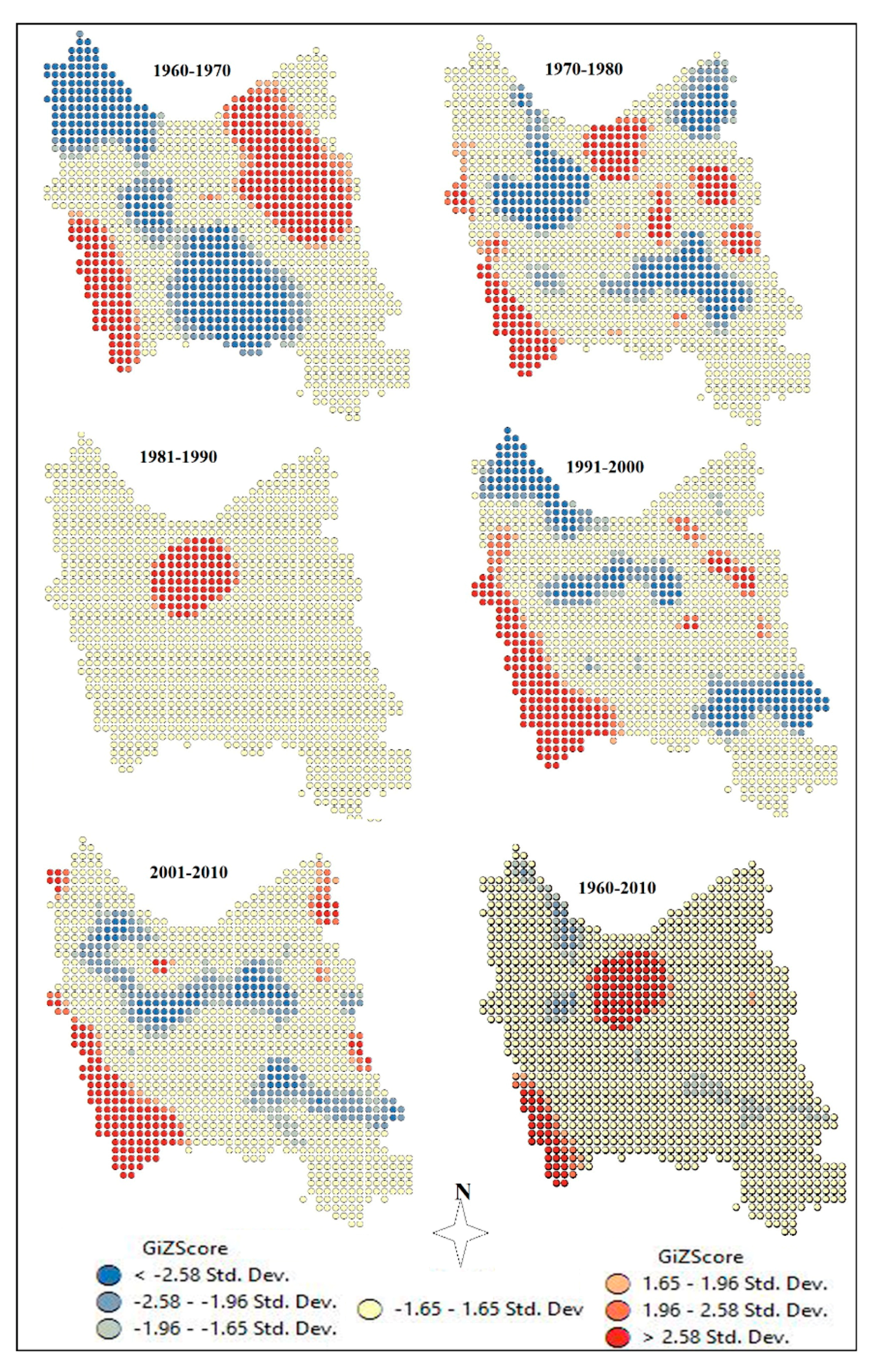
3.2. Analysis of Threshold Spatial Autocorrelation Pattern

In order to analyze the dominant pattern of extreme precipitation thresholds in the northwest of Iran, HOTSPOT analysis, known as Gi, was employed in this study. Gi is calculated for each phenomenon available in the data, which is a kind of Z score. With respect to positive, significant Z scores, higher Z scores show stronger clusters, hence the formation of hot spots. In other words, higher Z scores show high positive autocorrelation pattern. With regard to negative, significant Z scores, lower Z scores indicate stronger clustering of low values, i.e., the formation of cold spots or negative autocorrelation pattern. In order to obtain a better understanding of changes in the spatial autocorrelation pattern of extreme precipitation thresholds in the northwest of Iran, these patterns were extracted for the five decades. The results yielded clusters with high and low values (Figure 3).

In these figures, blue spots illustrate low clustering pattern or negative spatial autocorrelation pattern. Red spots, on the other hand, display high cluster pattern or positive spatial autocorrelation pattern. The grey spots show that these areas did not follow any specific spatial autocorrelation pattern. In the first decade, the low cluster pattern stretched from northwest to southeast. The spatial autocorrelation in this period is more in line with positive anomalies. That is, regions along Sahand and the Ghoosheh Dagh as well as some small areas of the southeast of the studied region have positive anomaly. However, no specific pattern dominated around 40% of the studied area. In addition, spatial patterns were more orderly in this period (

Table 3. Percentage of area covered with spatial autocorrelation pattern of extreme precipitation threshold in the northwest of Iran based on the spatial index of Gi.

	1961–1970	1971–1980	1981–1990	1991–2000	2001–2010	1961–2010
<−2.58 Std-Dev.	25.90521	12.00632	0	10.34755	4.344392	0
−2.58–−1.96 Std-Dev.	6.872038	6.240126	0	5.845182	10.11058	0.473934
−1.96–−1.65 Std-Dev.	3.080569	3.554502	0	3.00158	6.082148	4.186414
−1.65–1.65 Std-Dev.	39.17852	60.29384	91.46603	70.00316	68.60979	86.4613
1.65–1.96 Std-Dev.	0.157978	0.394945	0.078989	0.078989	0.157978	0.078989
1.96–2.58 Std-Dev.	3.974724	2.685624	0.157978	1.342812	0.947867	0.552923
>2.58 Std-Dev.	20.06319	15.08689	7.633491	9.636651	8.503949	8.766193

). Compared to the first decade, the dominant pattern of thresholds was less regular in the second decade, meaning that the pattern was irregularly distributed across the region. This irregular pattern may be attributed to the dominance of different systems in this period. Nevertheless, the intensity of low and high cluster patterns reduced in the second decade. Therefore, 12.01% of the studied region had low cluster pattern at the level of 99%. At the same time, positive spatial autocorrelation pattern experienced around 5% decline compared to the previous period (Table 3).

In the second decade, the intensity of positive and negative spatial autocorrelation decreased; however, more various systems dominated extreme precipitation thresholds in Iran. The influence of local factors should not be neglected either. Some researchers believe that harmonic-local systems explain over 90% of precipitation variations in the northwest of Iran [35]. In the third decade, the conditions that dominated thresholds were much more different. That is, the vast majority of the area (more than 90%) did not follow any particular pattern. In none of the regions of the studied area, thresholds did form low cluster pattern or negative spatial autocorrelation. Nevertheless, in around 8% of the studied area, which was mainly around the Ghoosheh Dagh, positive autocorrelation or high cluster pattern was observed. It is observed that the intensity of high cluster patterns reduced in recent decades. The area dominated by positive spatial autocorrelation declined by 2% in the third period (compared to the previous decade). In the fourth decade, the intensity of spatial autocorrelation pattern of extreme precipitation increased (compared to the previous period); however, it experienced a decline in comparison with the first two decades. More precisely, the area dominated by the pattern reduced by 11% and 4% for the first and second decades, respectively. Like the second decade, spatial autocorrelation pattern of the thresholds was dispersed across the area in the fourth decade. The fifth decade had more or less similar patterns to those of the previous one. Nevertheless, the area dominated by positive and negative anomalies reduced. It is concluded that, ignoring the third decade, the low and high cluster patterns of extreme precipitation thresholds experienced decline toward recent decades. On the other hand, the area of regions with no particular pattern increased. Thus, in the fifth decade, over 76% of the studied area did not follow any pattern of extreme precipitation threshold.

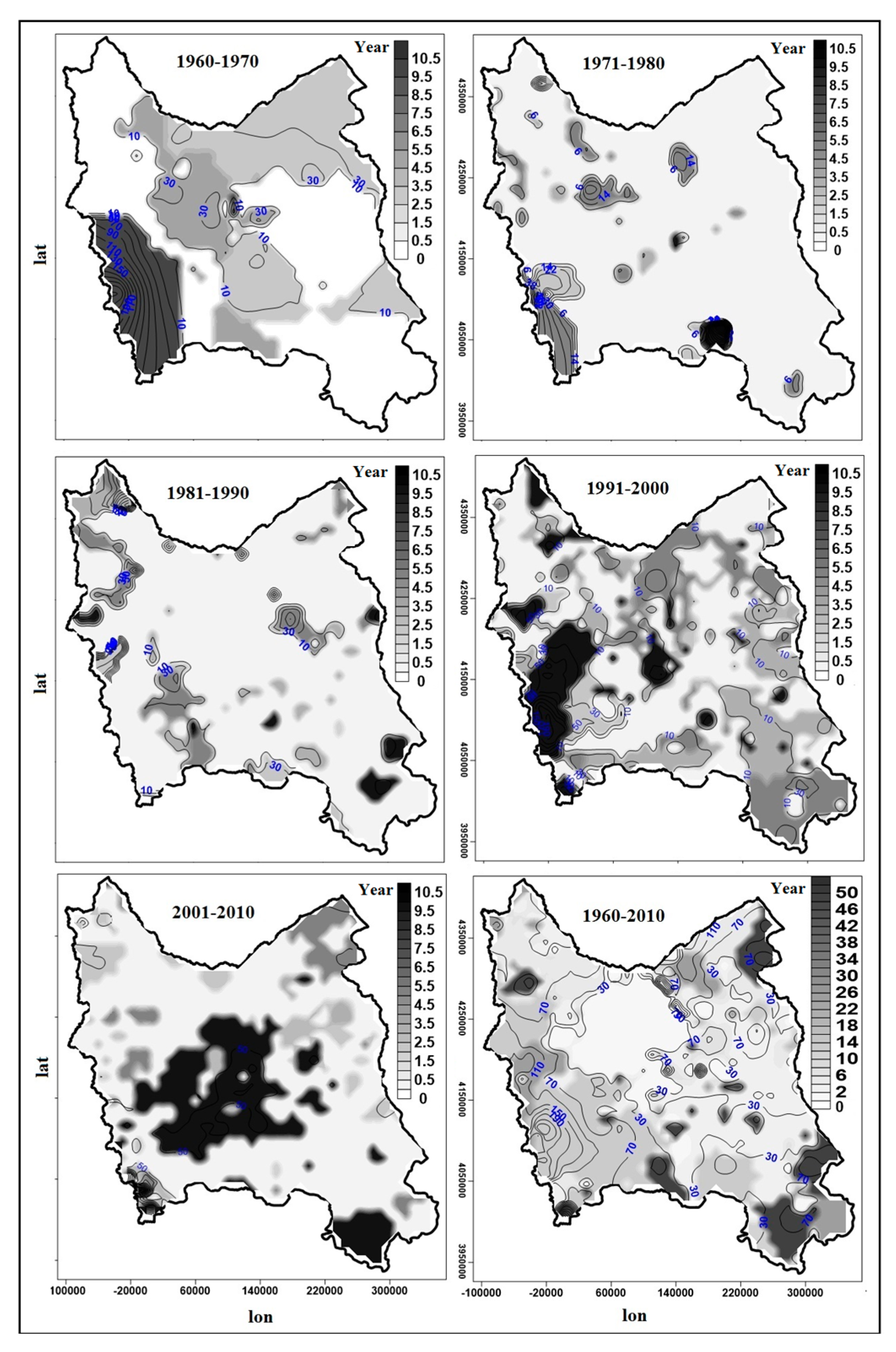
3.3. Analysis of Extreme Precipitation Threshold Patterns in the Northwest of Iran

Spectral analysis was conducted in order to further study decadal variations of extreme precipitation thresholds in the northwest of Iran. This analytical method is based on dividing the variance into time series or parts with various periods (or frequencies). It is a way of extracting and analyzing overt and covert oscillations with different wavelengths. Figure 3 shows the results of harmonic analysis of extreme precipitation thresholds in the northwest of Iran. In this procedure, after conducting harmonic analysis in each cell, first significant cycles with higher variances were extracted. In other words, the cycles which explained the largest proportion of the variance in every spot were selected. Cycle domains were determined in the light of the length of the studied period. For example, with regard to decadal cycle maps in which the length of the period was 10 years, cycles ranged from 0 to 10 years. Thus, the cycles in which the return period is as long as the studied period indicate a trend. In these figures, contours which have blue numbers display the variance of the studied cycles. It is observed that, in all the five decades, mainly short-term cycles dominated extreme precipitation thresholds in the northwest of Iran. In these figures, black spots illustrate cycles which are equal to the studied period. As mentioned above, these regions followed a trend. Therefore, in the first decade, 28.4% of the studied area had a return period of 2 to 4 years. Some researchers believe that these cycles can be explained in the light of El Nino. For instance, Serdar Kalayci et al. (2004) claimed that 2–5 year precipitation cycles in Turkey occur as a result of El Nino [48]. The majority of researchers believe that 2–4 year cycles can be attributed to El Nino Southern Oscillation (ENSO), large scale patterns of climate-ocean general circulation of the atmosphere, circuit currents, and other climate-ocean processes [49,50].

Comparison of figures of spatial pattern and cycle-related figures demonstrates that cycles with the highest variance occur along with the most intensive negative anomalies. Variety in circles shows changes in precipitation patterns (Figure 4). For examples, Jo and Lee (2010) believe that the variety of regional precipitation cycles in China are related to the southern monsoon flow in the east of China and western flow in the northwest of China [51]. In the fifth decade, 21.6% of the studied area, which mainly involves central regions of the area, had extreme precipitation threshold return cycles that were as long as the studied period. The number of these cycles was higher than that of other periods (

Table 4. Percentage of area covered by each cycle during the decades.

Cycle	1961–1970	1971–1980	1981–1990	1991–2000	2001–2010	1961–2010
0–2	42.7	86.9	81.1	44.5	60.7	46.1
2–4	28.4	4.1	8	23.9	10.9	18.7
4–6	12.6	8.2	8.4	18.6	6.7	1.7
6–8	0	0	0	0	0	24.4
>8	11.7	0.9	2.7	13	21.6	9.1

). In general, analysis of the annual cycle maps shows that the largest area of the studied region had short-term cycles. Mid-term cycles only constituted 24.4% of the studied area. Most scientists have attributed these cycles to El Niño—Southern Oscillations (ENSO) and Quasi Binomial Oscillations (QBOs)—atmospheric general circulation and zonal flows and other climate-ocean processes. Including, Torrence and Webster (1999) 2–3 year cycles in monsoon precipitation, Garcia et al. (2002), 2.7 year cycles in Iberia peninsula and Azad et al. (2009), 3–5 year cycles in Indian monsoon precipitation, are due to the impact of the ENSO [50,52,53]. Selvam and Joshi (1995), they discovered cycles of 2–7 years and cycles of 2–3 years at surface temperature and attributed these cycles respectively to the ENSO and QBOs [54].

In a study focusing on precipitation in the northwest of Iran, Razmi and Asakereh (2012) came to the same conclusion [35]. They revealed that there were sinusoidal cycles as long as 2–3, 3–5, 5–11 years or even longer than 11 years [35]. In total, in addition to above-mentioned cycles, 3–5 year cycles play an important role in the annual precipitation in this region. These cycles show the influence of ENSO on precipitation in this area. Cycles which are longer than 11 years in some small regions located in the southeast of this area and around Lake Urmia confirm Jahanbakhsh and Edalatdoost’s (2009) findings [55] (Figure 4). They concluded that the activity cycle of sunspots affect the precipitation frequency in Azerbaijan [55]. Study area’s precipitation cycles can be due to its location in lower boundary of the mid-latitude and adjacent to the subtropical high pressure [3,34,47].

4. Conclusions

Precipitation, which is the result of complex atmospheric interactions, is one of the most vital climatic events. Furthermore, compared to other climatic phenomena, it has a significantly more complicated behavior. Precipitation changes are the result of variation in factors that cause precipitation. Irregularity in these factors is also manifested in the distribution of spatial and temporal precipitation. Critical showers in various scales (especially on a daily basis) cause heavy damage to human society, especially in densely populated areas of the city and urban ecosystems. In order to establish a calm, stable life for humans and strike a balance in the environment, it is necessary to identify and study these natural hazards. The current study focused on investigating temporal and spatial variations in the anomalies, circles, and spatial autocorrelation pattern of extreme precipitation thresholds in the northwest of Iran. Data were collected from 250 stations of Iran’s Meteorological Organization for a 50-year period (1960–2010). The data were fed into MATLAB in order to extract the thresholds. The 99th percentile was used as the threshold of extreme precipitation. In order to analyze threshold cycles and spatial autocorrelation pattern changes, harmonic analysis and Gi were used respectively. With the aim of gaining a better understanding of thresholds, the obtained thresholds were analyzed within five equal periods (1960–1970, 1971–1980, 1981–1990, 1991–2000, and 2001–2010). Spatial distribution of mean scores showed that, during the five decades, the majority of the studied area had a mean threshold of 6 to 8 mm. In the third period, however, a considerable increase was observed in the thresholds. Therefore, in this decade, thresholds significantly went up in highland regions, especially along Sabalan and the Ghoosheh Dagh. The results obtained through Gi analysis further support this claim. In addition, spatial analysis of HOTSPOT index revealed no dominant negative spatial autocorrelation pattern in the extreme precipitation threshold in the northwest of Iran. The extreme precipitation thresholds have decreased in recent periods (fourth and fifth). However, the spatial distribution of thresholds is more uniform than in previous periods. Spatial Distribution of abnormalities of extreme precipitation thresholds in all periods complies with the spatial distribution of heights, so that the highlands have a positive anomaly and the lower regions have a negative anomaly. The third period has the most fluctuating anomalies, so that more than 80% of the studied area has a negative anomaly. The results also show that spatial autocorrelation patterns of extreme precipitation thresholds were more regular in the first period. In the second period, the severity of positive and negative spatial autocorrelation patterns was reduced and in the third period the majority of the study area did not have a pattern.

In general, towards the recent periods, the area of positive and negative spatial autocorrelation patterns has been reduced. However, the results indicate that, during the first period (1960–1970), there was a concentration of spatial patterns, hence extreme precipitation thresholds were influenced by external factors. From the third decade on, spatial patterns were dispersed, meaning that extreme precipitation thresholds were mainly influenced by local factors, especially in highlands. On the other hand, the dispersion of the spatial patterns of extreme precipitation may indicate that, over the past few years, atmospheric patterns governing these thresholds, under the influence of climate change, they have had irregular patterns. Therefore, it can be concluded that the regularity of the effective patterns on the extreme precipitation thresholds of the northwest of Iran is very irregular and has high fluctuations.

The results of analyzing oscillations of extreme precipitation thresholds in the northwest of Iran showed that, on decade- and year-based scales, extreme precipitation thresholds were largely dominated by short-term cycles of 2 to 4 years. And after that, the mid-term cycles have dominated the studied area. Most scientists have attributed these cycles to ENSO and Qusi-Biennial Oscillations (QBO) of the large-scale pattern of climate-ocean general circulation of the atmosphere, circuit currents, and other climate-ocean processes [56,57]. However, there were regions that extreme precipitation thresholds have cycles equivalent to the length of the statistical period, which indicate that there is the trend in the data. Also, the most diverse cycles are consistent with the most severe negative abnormalities that could be due to changes in precipitation patterns in the studied area.

References

1. Data, C. Guidelines on Analysis of Extremes in A Changing Climate in Support of Informed Decisions for Adaptation. Available online: http://www.wmo.int/pages/prog/wcp/wcdmp/wcdmp_series/documents/WCDMP_72_TD_1500_en__1.pdf (accessed on 4 June 2017).
2. Rousta, I.; Doostkamian, M.; Haghighi, E.; Mirzakhani, B. Statistical-synoptic analysis of the atmosphere thickness pattern of iran’s pervasive frosts. Climate 2016, 4, 41. [Google Scholar] [CrossRef]
3. Alijani, B.; Doostkamyan, M.; Bayat, A.; Balyani, Y.; Javanmard, A. Analysis of precipitation in iran. In The Second International Conference on Environmental Hazards; Khuarazmi University Press: Tehran, Iran, 2013; Volume 2, p. 220. [Google Scholar]
4. Rousta, I.; Khosh Akhlagh, F.; Soltani, M.; Modir Taheri Sh, S. Assessment of blocking effects on rainfall in northwestern iran. In Comecap 2014; COMECAP: Heraklion, Grecce, 2014; Volume 1, pp. 127–132. [Google Scholar]
5. Masoudian, S.A.; Kaviani, M.R. Climatology of Iran; Isfahan University Press: Isfahan, Iran, 2007; Volume 1. [Google Scholar]
6. Martin, G.; Ringer, M.; Pope, V.; Jones, A.; Dearden, C.; Hinton, T. The physical properties of the atmosphere in the new hadley centre global environmental model (Hadgem1). Part I: Model description and global climatology. J. Clim. 2006, 19, 1274–1301. [Google Scholar] [CrossRef]
7. Lohmann, U.; Rotstayn, L.; Storelvmo, T.; Jones, A.; Menon, S.; Quaas, J.; Ekman, A.M.; Koch, D.; Ruedy, R. Total aerosol effect: Radiative forcing or radiative flux perturbation? Atmos. Chem. Phys. 2010, 10, 3235–3246. [Google Scholar] [CrossRef]
8. Asakereh, H. Frequency distribution change of extreme precipitation in zanjan city. Geogr. Environ. Plan. 2012, 23, 51–66. [Google Scholar]
9. Andrews, T.; Forster, P.M.; Gregory, J.M. A surface energy perspective on climate change. J. Clim. 2009, 22, 2557–2570. [Google Scholar] [CrossRef]
10. Andrews, T.; Forster, P.M.; Boucher, O.; Bellouin, N.; Jones, A. Precipitation, radiative forcing and global temperature change. Geophys. Res. Lett. 2010, 37, 1–6. [Google Scholar] [CrossRef]
11. Eriyagama, N.; Smakhtin, V.; Chandrapala, L.; Fernando, K. Impacts of Climate Change on Water Resources and Agriculture in Sri Lanka: A Review and Preliminary Vulnerability Mapping; IWMI: Colombo, Sri Lanka, 2010; Volume 135. [Google Scholar]
12. Verner, D.; Lee, D.; Ashwill, M. Increasing Resilience to Climate Change in the Agricultural Sector of the Middle East: The Cases of Jordan and Lebanon; World Bank Publications: Washington, DC, USA, 2013. [Google Scholar]
13. Knapp, A.K.; Beier, C.; Briske, D.D.; Classen, A.T.; Luo, Y.; Reichstein, M.; Smith, M.D.; Smith, S.D.; Bell, J.E.; Fay, P.A.; et al. Consequences of more extreme precipitation regimes for terrestrial ecosystems. BioScience 2008, 58, 811–821. [Google Scholar] [CrossRef]
14. Groisman, P.Y.; Knight, R.W.; Easterling, D.R.; Karl, T.R.; Hegerl, G.C.; Razuvaev, V.N. Trends in intense precipitation in the climate record. J. Clim. 2005, 18, 1326–1350. [Google Scholar] [CrossRef]
15. New, M.; Todd, M.; Hulme, M.; Jones, P. Precipitation measurements and trends in the twentieth century. Int. J. Climatol. 2001, 21, 1889–1922. [Google Scholar] [CrossRef]
16. Zahran, M.A. Afro-asian mediterranean coastal lands. In Climate—Vegetation: Afro-Asian Mediterranean and Red Sea Coastal Lands; Gilbert, F., Ed.; Springer: Dordrecht, The Netherlands, 2010; pp. 1–103. [Google Scholar]
17. Alexander, L.; Zhang, X.; Peterson, T.; Caesar, J.; Gleason, B.; Klein Tank, A.; Haylock, M.; Collins, D.; Trewin, B.; Rahimzadeh, F. Global observed changes in daily climate extremes of temperature and precipitation. J. Geophys. Res. Atmos. 2006, 111, 1–22. [Google Scholar] [CrossRef]
18. Bordi, I.; Fraedrich, K.; Petitta, M.; Sutera, A. Extreme value analysis of wet and dry periods in sicily. Theor. Appl. Climatol. 2007, 87, 61–71. [Google Scholar] [CrossRef]
19. Sen Roy, S. A spatial analysis of extreme hourly precipitation patterns in india. Int. J. Climatol. 2009, 29, 345–355. [Google Scholar] [CrossRef]
20. Sugahara, S.; Da Rocha, R.P.; Silveira, R. Non-stationary frequency analysis of extreme daily rainfall in sao paulo, brazil. Int. J. Climatol. 2009, 29, 1339–1349. [Google Scholar] [CrossRef]
21. Łupikasza, E.B.; Hänsel, S.; Matschullat, J. Regional and seasonal variability of extreme precipitation trends in southern poland and central-eastern germany 1951–2006. Int. J. Climatol. 2011, 31, 2249–2271. [Google Scholar] [CrossRef]
22. Wüest, M.; Frei, C.; Altenhoff, A.; Hagen, M.; Litschi, M.; Schär, C. A gridded hourly precipitation dataset for switzerland using rain-gauge analysis and radar-based disaggregation. Int. J. Climatol. 2010, 30, 1764–1775. [Google Scholar] [CrossRef] [Green Version]
23. Hand, W.H.; Fox, N.I.; Collier, C.G. A study of twentieth-century extreme rainfall events in the United Kingdom with implications for forecasting. Meteorol. Appl. 2004, 11, 15–31. [Google Scholar] [CrossRef]
24. Unkašević, M. Statistical analysis of daily maximum and monthly precipitation at Belgrade. Theor. Appl. Climatol. 2000, 66, 241–249. [Google Scholar] [CrossRef]
25. Seibert, P.; Frank, A.; Formayer, H. Synoptic and regional patterns of heavy precipitation in Austria. Theor. Appl. Climatol. 2007, 87, 139–153. [Google Scholar] [CrossRef]
26. Mätlik, O.; Post, P. Synoptic weather types that have caused heavy precipitation in Estonia in the period 1961–2005. Estonian J. Eng. 2008, 14, 195–208. [Google Scholar]
27. Soltani, M.; Laux, P.; Kunstmann, H.; Stan, K.; Sohrabi, M.; Molanejad, M.; Sabziparvar, A.; SaadatAbadi, A.R.; Ranjbar, F.; Rousta, I. Assessment of climate variations in temperature and precipitation extreme events over Iran. Theor. Appl. Climatol. 2016, 126, 775–795. [Google Scholar] [CrossRef]
28. Rahimzadeh, F.; Asgari, A.; Fattahi, E. Variability of extreme temperature and precipitation in Iran during recent decades. Int. J. Climatol. 2009, 29, 329–343. [Google Scholar] [CrossRef]
29. Rousta, I.; Soltani, M.; Zhou, W.; Cheung, H.H. Analysis of extreme precipitation events over central plateau of Iran. Am. J. Clim. Chang. 2016, 5, 297. [Google Scholar] [CrossRef]
30. Zolfagari, H.; Hashemi, R.; Fashi, M. The proportion of daily maximum precipitation to annual precipitation in Iran. Geogr. Res. Q. 2010, 92, 165–188. [Google Scholar]
31. Rousta, I.; Doostkamian, M.; Haghighi, E.; Ghafarian Malamiri, H.R.; Yarahmadi, P. Analysis of spatial autocorrelation patterns of heavy and super-heavy rainfall in Iran. Adv. Atmos. Sci. 2017, 34, 1069–1081. [Google Scholar]
32. Soltani, M.; Rousta, I.; Khosh Akhlagh, F.; Modir Taheri Sh, S. Statistical synoptic analysis of summertime extreme precipitation events over Kerman Province, Iran. In COMECAP 2014; COMECAP: Heraklion, Grecce, 2014; Volume 1, pp. 164–169. [Google Scholar]
33. Soltani, M.; Rousta, I.; Taheri, S.S.M. Using mann-kendall and time series techniques for statistical analysis of long-term precipitation in gorgan weather station. World Appl. Sci. J. 2013, 28, 902–908. [Google Scholar]
34. Alijani, B. Spatial analysis of critical temperatures and daily precipitation in Iran. J. Geogr. Sci. Appl. Res. 2011, 20, 9–30. [Google Scholar]
35. Razmi, R.; Asakereh, H.; Asakereh, H. Analysis of annual precipitation changes in northwest of Iran. Geogr. Environ. Plan. 2012, 23, 147–162. [Google Scholar]
36. Asakereh, H.; Doostkamian, M.; Sadrafshary, S. Anomalies and cycles of precipitable water over Iran in recent decades. Arab. J. Geosci. 2015, 11, 9569–9576. [Google Scholar] [CrossRef]
37. Asakereh, H. Trends in monthly precipitation over the northwest of Iran (Nwi). Theor. Appl. Climatol. 2016. [Google Scholar] [CrossRef]
38. Mohammadi, H.; Azizi, G.; khoshahklagh, F.; Ranjbar, F. Analysis of daily precipitation extreme indices trend in Iran. Phys. Geogr. Res. Q. 2017, 49, 21–37. [Google Scholar]
39. Jahahnbakhsh Asl, S.; Mirhashemi, H.; Tadayyon, M. Synoptic and thermodynamic analysis, the heavy in north west of Iran (East Azarbaijan Province). Geogr. Plan. 2015, 19, 107–125. [Google Scholar]
40. Mehdinasab, M.; Tavousi, T.; Mirzaei, R. Prediction probable flood and maximum precipitation using poldukhtar basin suffered partial series. Iran’s Nat. Ecosyst. 2014, 5, 97–109. [Google Scholar]
41. Moghbel, M.; Davodi, M.; Naistani, A.; Taghavi, F. Identify changes in iran’s precipitation regime in recent decades. NIVAR 2011, 35, 55–66. [Google Scholar]
42. Javari, M. Spatial variability of rainfall trends in Iran. Arab. J. Geosci. 2017, 10, 78. [Google Scholar] [CrossRef]
43. George, R. A new approach to time series with mixed spectra. Available online: https://statistics.stanford.edu/sites/default/files/PAR%20NSF%2014.pdf (accessed on 4 June 2017).
44. Lee, J.; Wong, D.W.S. Statistical Analysis with Arcview Gis; Wiley: Hoboken, NJ, USA, 2001. [Google Scholar]
45. Wilks, D.S. Statistical Methods in the Atmospheric Sciences; Academic Press: Cambridge, MA, USA, 2011. [Google Scholar]
46. Masoodian, S.; Mohammadi, B. The analysis of frontogenesis frequency at time of super heavy rainfall in Iran. Geogr. Res. 2012, 27, 1–23. [Google Scholar]
47. Alijani, B. The Climate of Iran; Payam Noor University Press: Tehran, Iran, 1995; p. 230. [Google Scholar]
48. Kalayci, S.; Karabörk, M.; Kahya, E. Analysis of El Nino signals on Turkish streamflow and precipitation patterns using spectral analysis. Fresenius Environ. Bull. 2004, 13, 719–725. [Google Scholar]
49. Hartmann, H.; Becker, S.; King, L. Quasi-periodicities in Chinese precipitation time series. Theor. Appl. Climatol. 2008, 92, 155–163. [Google Scholar] [CrossRef]
50. García, J.; Serrano, A.; De la Cruz Gallego, M. A spectral analysis of Iberian Peninsula monthly rainfall. Theor. Appl. Climatol. 2002, 71, 77–95. [Google Scholar] [CrossRef]
51. Jo, Y.-J.; Lee, J.-Y. Time series analysis of hydrologic data obtained from a man-made undersea Lpg cavern. Eng. Geol. 2010, 113, 70–80. [Google Scholar] [CrossRef]
52. Torrence, C.; Webster, P.J. Interdecadal changes in the enso–monsoon system. J. Clim. 1999, 12, 2679–2690. [Google Scholar] [CrossRef]
53. Azad, S.; Vignesh, T.; Narasimha, R. Periodicities in Indian monsoon rainfall over spectrally homogeneous regions. Int. J. Climatol. 2010, 30, 2289–2298. [Google Scholar] [CrossRef]
54. Selvam, A.M.; Joshi, R. Universal spectrum for interannual variability in Coads global air and sea-surface temperatures. Int. J. Climatol. 1995, 15, 613–623. [Google Scholar] [CrossRef]
55. Jahanbakhsh, S.; Edalat, D.M. Study of climate change in Iran (case study: North atlantic oscillation as an indicator of the impact of solar activity on changes in precipitation of Azerbaijan region). In Third International Conference on Iran’s Water Resources Management Iran; School of Civil Engineering: Tabriz, Iran, 2009; Volume 1, p. 325. [Google Scholar]
56. Lana, X.; Martínez, M.; Serra, C.; Burgueño, A. Periodicities and irregularities of indices describing the daily pluviometric regime of the Fabra Observatory (Ne Spain) for the years 1917–1999. Theor. Appl. Climatol. 2005, 82, 183–198. [Google Scholar] [CrossRef]
57. Kane, R.P.; Teixeira, N.R. Power spectrum analysis of the annual rainfall series for Massachusetts (Ne, USA). Clim. Chang. 1991, 18, 89–94. [Google Scholar] [CrossRef]
Figure 1. Height and distribution of stations in the northwest of Iran.
Atmosphere 08 00135 g001
Figure 2. Spatial distribution of mean, weighted mean center, and anomalies of extreme precipitation thresholds.
Atmosphere 08 00135 g002
Figure 3. Spatial autocorrelation pattern of extreme precipitation thresholds in the northwest of Iran based on the spatial index of Gi.
Atmosphere 08 00135 g003
Figure 4. Spatial distribution of return period and variance of extreme precipitation thresholds in the northwest of Iran.
Atmosphere 08 00135 g004