Estimation of the Elemental to Organic Carbon Ratio in Biomass Burning Aerosol Using AERONET Retrievals

1. Introduction

It is well established that aerosol released from open biomass burning (BB) has a substantial impact on global climate processes due to both absorption and scattering of incoming solar shortwave radiation [1], as well as due to aerosol-cloud interactions [2,3]. BB aerosol is also known to have a considerable effect on air quality in regions that are episodically affected by wildfires (e.g., [4,5,6]).

A balance between the cooling and warming effects of BB aerosol critically depends on the ratio of the major absorbing and scattering aerosol components contributing the radiative forcing of opposite sign, such as elemental or black carbon (EC or BC) and organic carbon (OC) [7]. As the available modeling estimates of the contribution of BB aerosol to radiative forcing are presently rather uncertain [8], a good knowledge of the EC/OC ratio in BB aerosol is therefore an important prerequisite for reducing uncertainties in the modeling analysis of the climate effects of BB aerosol. There is evidence [9,10,11,12] that knowledge of the EC/OC ratio in BB aerosol may also help to improve model representations of the absorption caused by organic compounds constituting the so-called brown carbon (BrC), which, along with EC (or BC), contributes significantly to the BB aerosol radiative forcing [13,14,15]. Unlike EC, BrC is subject to photochemical aging or may be formed as secondary species from primary gaseous emissions [16]. Similarly, any observational constraints to the partitioning between EC and OC may be beneficial for improving model representations of organic aerosol mass, which (again unlike EC) is prone to significant changes during the atmospheric evolution of BB aerosol [17,18,19,20], in the context of air pollution modeling applications. (Note that the distinction made in the literature between EC and BC mostly reflects the differences between specific measurement techniques [7,21] and is not so important here. For consistency, the former term (EC) is mostly used throughout this paper, unless otherwise necessary in a given context).

The partitioning between EC and OC in models simulating BB aerosol composition is usually based on data of fire emission inventories, such as, e.g., the Global Fire Emissions Database (GFED) [22], the Fire INventory from NCAR (FINN) [23] or the Global Fire Assimilation System (GFAS) [24], which employ available in situ measurements of the emission factors to calculate emissions of individual species on regional and global scales. However, due to variations in combustion conditions and in fuel origin, moisture and geometry, different measurements yield a wide range of emission factor values, even when they are made in similar climate zones and types of environment [25]. As a result of large variations in the emission factors for EC and OC, the uncertainty of typical values of the EC/OC ratio may considerably exceed a factor of two for BB aerosol in extratropical forest and a factor of four in savanna and grassland [26,27]. It seems reasonable to expect that the uncertainties in the emission factors for EC and OC assumed in the fire emission inventories are especially large in the case of fires in such a remote region as Siberia due to the lack of dedicated local measurements.

Siberia represents one of the world’s largest forested regions [28,29]. Devastating Siberian fires are known to considerably affect the composition of the atmosphere over vast territories in Russia [30], with smoke plumes reaching Japan, Korea and even North America [31,32,33]. Emissions from Siberian fires are also found to provide a major source of EC deposited in the Arctic [34], thus contributing to rapid warming observed there [35]. As the on-going global warming is likely to lead to increases in the probability and intensity of fires in the boreal forest, there is a need to better understand and quantify emissions from Siberian fires and possible complex feedbacks between Siberian fires and their effects on regional and global climate [36,37,38]. In view of these challenges, it is particularly important to ensure that predictions of the composition and optical properties of BB aerosol originating from boreal fires by climate and chemistry transport models are sufficiently adequate.

Consistent and abundant data on BB aerosol optical properties worldwide are available presently as inversion products from measurements performed by the ground-based Sun photometers at the Aerosol Robotic Network (AERONET) sites [39]. Several AERONET sites are located in the Siberian region. The aerosol absorption optical depth (AAOD) and single scattering albedo (SSA) retrieved from the AERONET measurements [40] are extensively used to evaluate and constrain the aerosol light absorption and atmospheric EC (BC) amounts simulated with models (e.g., [41,42,43,44,45]). Another promising source of aerosol light absorption data that can be used to constrain the models is the AAOD retrievals from satellite measurements [46]. For example, the OMI (Ozone Monitoring Instrument) observations of AAOD at the 388-nm wavelength were proven to be useful in improving simulations with a global chemistry transport model and in reducing uncertainties in BC emissions in Southeast Asia [47].

A major obstacle in interpretation and addressing the discrepancies between the model and measurement AAOD data (note that the models were typically found to strongly underestimate AAOD) is that the modeled relationship between the atmospheric EC amounts and AAOD is very sensitive to the assumptions and simplifications regarding the mixing state of aerosol and intensive optical properties (such as, e.g., the absorption Ångström exponent and the refractive index) of its individual constituents, including EC and organic compounds [7,48]. One of the available approaches to overcoming this obstacle involves constraining the contribution of EC to aerosol light absorption by using the multi-wavelength absorption measurements and taking into account the fact that the absorption Ångström exponent (AAE) for EC is different from AAE of other aerosol components (including BrC and dust). Multiple studies (e.g., [11,15,49,50,51]) followed this approach in the analysis of field measurements and remote sensing aerosol absorption data by using different AAE-based methods. However, although such methods proved to be useful in constraining absorption of EC and BrC, they typically do not provide a direct inference on the EC/OC mass ratio in aerosol particles.

Another measurement-based approach to constraining EC absorption involves parameterization of the aerosol absorption properties as a function of the aerosol chemical composition. Specifically, it was shown [9,10] that the imaginary part of the refractive index for organic BB aerosol can be parameterized as a growing function of the EC/OC ratio. More recently, as a result of the analysis of optical properties and the composition of BB aerosol formed from a wide range of wildland fuels from North America, it was demonstrated [52] that there is a linear relationship between the EC/(EC + OC) ratio and SSA at several visible wavelengths (405, 532 and 660 nm).

In this study, we combine the AERONET multi-wavelength absorption measurements made in Siberia during the extreme summer fire season of 2012 [20,30] and the empirical relationships [52] between SSA and the EC/OC ratio. Our primary goal is to obtain measurement-based estimates of the EC/OC ratio for BB aerosol in Siberia and to use them for the evaluation of the corresponding simulations performed with a regional chemistry transport model involving EC and OC emission factors used in the GFED inventory. Another goal of this study is to develop a parameterization enabling estimation of the EC/OC mass ratio using a combination of data from available satellite measurements, such as AAOD retrieved from the OMI measurements [46] and extinction aerosol optical depth (AOD) from the MODIS (Moderate Resolution Imaging Spectroradiometer) [53] measurements. The parameterization is intended to contribute to the methodological basis for possible prospective inverse modeling studies aimed at constraining EC emissions from boreal wildfires using satellite observations.

2. Data and Method

2.1. Measurement and Model Data

2.1.1. Measurements

We use the aerosol SSA data provided by AERONET as the Version 2, Level-2 (cloud screened and quality assured) aerosol inversion product [40]. We also utilize AOD data available as the Version 2, Level-2 direct sun AERONET observations [39]. The data representing aerosol properties in the total atmospheric column were retrieved from diffuse sky radiance and direct sun radiance measurements performed by Cimel Electronique sun photometers and are publicly available for downloading from the AERONET website [54]. We use SSA observations at the 440-, 675- and 869-nm wavelengths and AOD values for the 440- and 500-nm wavelengths.

In our analysis, we consider the AERONET data available for the period of summer months (June–August) of 2012 from the Tomsk-22 (56°25′01″ N, 84°04′26″ E) and Yakutsk (61°39′43″ N, 129°22′01″ E) sites situated in Siberia. Unfortunately, the multi-day Level-2 SSA data for the fire season of 2012 were not available from any other Siberian stations. Furthermore, there were almost no data available from the Tomsk-22 and Yakutsk stations for spring and fall months of 2012.

To obtain estimates of the EC/OC ratio, we selected the SSA retrievals satisfying three criteria (see

Table 1. Selection criteria applied to the AERONET observations. BB, biomass burning.

Criterion No.	Selection Parameter	Threshold Value
1	Aerosol optical depth 1 at 500 nm	0.5
2	Relative humidity 2 in the BB aerosol column	60%
3	BB aerosol photochemical age 2	30 h

¹ According to the AERONET observations; ² according to the simulations with the CHIMERE model.

). First, it was required that AOD at 500 nm exceeds the value of 0.5. Taking into account the corresponding model results (see Section 3), this AOD value was chosen as an indicator of a predominant contribution of biomass burning to aerosol observed in almost pristine conditions of Siberian boreal forest. The second selection criterion was introduced to exclude situations where aerosol optical properties might be significantly affected by humidification of aerosol particles. Specifically, based on available studies of the effects of humidity on BB aerosol (e.g., [55,56]), we disregarded the observed cases where the average relative humidity (RH) in the aerosol column was greater than 60%. Values of RH were evaluated as described below in Section 2.1.2. Finally, the third selection criterion was introduced to minimize the possibility that observed aerosol optical properties are strongly affected by changes in particle morphology and composition that may occur [57,58] as a result of atmospheric aging of BB aerosol. The selection was based on our estimates of the photochemical age of BB aerosol (see Section 2.1.2): observations of aerosol aged more than 30 h were excluded from the analysis. While choosing the threshold age value (which, ideally, should be as small as possible), we tried to ensure that the amount of the remaining data would be sufficient for statistical inferences. With the current choice (30 h), our analysis involved 20 observations (including 14 and 6 observations at the Tomsk-22 and Yakutsk sites, respectively), while nearly the same amount of available observations (from the both stations considered) satisfying the two other criteria were disregarded.

Note that one of the major screening criteria originally applied by AERONET to inversion data comprising the Level-2 product is that AOD at 440 nm (AOD⁴⁴⁰) must not be less than 0.4. This criterion allows constraining the error of SSA retrievals [59], but at the expense of the invalidation of many SSA retrievals, which are otherwise available as the Level-1.5 inversion product [60]. The uncertainty in the SSA retrievals in situations with prevailing BB aerosol was estimated to be ±0.03 [59] when AOD⁴⁴⁰ is larger or equal to 0.5.

In this study, we also utilized the Fire Radiative Power (FRP) data derived from the MODIS satellite measurements [61]. The FRP data were obtained as the Collection 6 Level 2 active fire product through the Reverb metadata discovery tool [62] and were used to specify BB emissions for our simulations described below.

2.1.2. Simulations

The model data play a supplementary, but still significant role in this study, being used for the justification of the criterion applied to select observations representative of BB aerosol, for estimation of the BB aerosol age and for the comparison with the EC/OC ratios derived from the AERONET measurements. The simulations were performed with the CHIMERE chemistry transport model (CTM) [63]. Similar simulations were employed in the framework of our previous studies of atmospheric effects of Siberian fires [20,30]. For this reason, we describe our simulations only briefly, focusing on modifications and differences with respect to earlier studies.

In this study, the simulations were performed with one of the latest CHIMERE versions (v2016, http://www.lmd.polytechnique.fr/chimere/CW-chimdev.php) [64]. An important feature of that model version is online calculations of photolysis rates with the Fast-JX scheme enabling representation of optical effects of aerosols and clouds and estimation of AOD. The optical calculations in CHIMERE are based on the Mie theory and make use of a pre-described set of typical values of the refractive index for all aerosol species, including EC and OC. Our simulations were configured by using mostly the “recommended values” of input parameters as specified in the CHIMERE documentation [65]; otherwise, the simulation settings are described below.

The simulations addressed the atmospheric evolution of several types of aerosol, including dust, biomass burning, anthropogenic, biogenic and sea salt aerosols, and of a number of minor gaseous species affecting the oxidation potential and secondary aerosol formation in the lower atmosphere. The aerosol dynamics was simulated using the sectional approach with 10 bins covering the range of particle sizes from 10 nm–40 µm. Organic aerosol (OA) evolution was represented in the simulations by taking into account both its primary and secondary fractions: the primary OA was assumed to be composed of nonvolatile material, while the secondary OA (SOA) was formed as a result of a single step oxidation of aromatic and biogenic VOC precursors; note that the representation of OA evolution in this study was the same as in the “STN” (“standard”) model runs performed in our previous studies [19,20].

Anthropogenic emissions of aerosol and gases were specified using monthly emission data for the year 2010 from the global HTAP (Hemispheric Transport of Air Pollution) v2 emission inventory [66] and the CHIMERE standard emission interface. The HTAP data for the year 2010 were used because the corresponding 2012 data were not available; we presume that changes in annual anthropogenic emissions in the Siberian region could hardly be considerable during the period of three years and can be disregarded. The BB emissions were estimated using the FRP observations mentioned above by applying to them, sequentially, the FRP to biomass burning rate conversion factor and the emission factors (species and land cover dependent). The methodology used to process and re-grid the FRP data, as well as the procedure aimed at the estimation of the conversion factor relating FRP and biomass burning rate values were developed earlier and are described elsewhere [4,30,67].

In this study, the conversion factor was calibrated by minimizing the root mean square difference between the AOD values obtained from CHIMERE for the 500-nm wavelength and corresponding AOD values available from the AERONET sites considered (see Section 2.1.1) for summer months of 2012. The optimal value of the conversion factor was found to be 6.81 × 10⁻⁴ g s⁻¹ W⁻¹. For comparison, a similar calibration procedure applied earlier to the satellite AOD data in the same region yielded a 40% larger value of the conversion factor [20]. The difference may, in particular, be due to spatial and temporal inhomogeneity in burning conditions, as well as due to the fact that the previous study [20] utilized the Collection 5 fire data product, while the more recent Collection 6 data were used in this study. The emission factors for aerosol and gaseous species used in this study were specified using the recommended emission factor values for boreal forest, savanna and agricultural fires from the GFED4 (Global Fire Emissions Database) emission inventory [68]. The EC/OC ratios in BB aerosol emissions were accordingly assumed to be of 0.052, 0.14 and 0.32 for boreal forest, savanna (including both grass and bush) and agricultural fires, respectively.

To enable estimation of the photochemical age of BB aerosol, the standard CHIMERE simulations were extended (similarly as was done previously [20]) to include two special tracers. While the first tracer (T_p) was chemically passive, the second tracer (T_r) reacted with OH (without consuming it). The reaction rate (k_OH) in this case was 9 × 10⁻¹² s⁻¹ cm³. Again similarly to the method proposed earlier [20], the photochemical age of BB aerosol in the atmospheric column at a given location was estimated using the ratio of the mass column concentrations, [T_p] and [T_r], of the corresponding tracers:

$$t_a=-{(k_{\mathrm{OH}}[\mathrm{OH}\left]\right)}^{-1}\ln \left([{\mathrm{T}}_r]/[{\mathrm{T}}_p]\right)$$

(1)

where [OH] is the weighted vertical mean OH concentration at the location and time of the AERONET measurements, with the weights proportional to concentration of the inert tracer T_p. Note that a similar estimation described earlier [20] involved constant (typical) OH concentration (independent of location and time). Variations in OH concentration may be due to the variability of the density of BB plumes and typically increases as AOD increases. Therefore, on the one hand, allowing for variations of OH concentration in Equation (1) may enable more realistic estimates of the BB aerosol photochemical age in view of a probable large variability in density of young BB plumes. However, on the other hand, using OH concentration corresponding to aged (and thus, dispersed) plumes is likely to result in overestimation of the photochemical age. A comparison of the photochemical age estimated using Equation (1) with the duration of daylight on the days when the AERONET measurements selected for this study were made indicated that Equation (1) applied to the data analyzed here typically overestimates the photochemical age by about 30%.

We used the model domain covering Siberia and parts of European Russia and the Russian Far East (48° N–66° N; 20° E–56° E) with a horizontal resolution of 1.0° × 1.0°. The model grid had 12 non-equidistant levels, with the top of the upper level fixed at 200 hPa. The simulations were done for the period of four months (May–August) of 2012, with the model’s spin-up period comprising the initial month. The CHIMERE runs were driven with meteorological data provided by the WRF (Weather Research and Forecasting) (v.3.6, http://www.wrf-model.org/index.php) model [69] configured as described earlier [20]. The same meteorological model provided RH values employed in the data selection procedure (see Section 2.1.1): RH in the BB aerosol columns was calculated as a weighted vertical average of the local RH values, with the T_p concentration used as the weights. Separate simulations (labeled below as “fire” and “bgr”) were performed with and without fire emissions. The contribution of fires to EC or OC concentrations and AOD were evaluated as the difference between the corresponding values predicted by these simulations.

2.2. Method for Estimation of the EC/OC Ratio

Our estimation procedure is based on recent findings [52] from the Fourth Fire Laboratory at Missoula Experiment (FLAME-4), which involved burning of a wide variety of biomass fuels and measuring absorption properties of the produced fresh aerosol at several wavelengths (660, 532 and 405 nm). It has been shown, specifically, that BB aerosol particle SSA (denoted in the formulations given below as ω₀) can be parameterized as a linear function of the elemental to total carbon ratio:

$${\omega }_0^{\lambda }\cong a^{\lambda }\frac{[EC]}{[EC]+[OC]}+b^{\lambda }$$

(2)

Here and below, ${\omega }_0^{\lambda }$ is SSA at a given wavelength λ; [EC] and [OC] are the mass concentrations of the corresponding species; and a^λ and b^λ are constant positive parameters depending on the wavelength, λ. Values of a^λ and b^λ that have been reported [52] for optimal fits to the FLAME-4 data are listed in

Table 2. The coefficients of the linear regressions relating single scattering albedo (SSA) at different wavelengths, λ, as the dependent variable to the EC/(EC + OC) ratio (see Equation (2)). The regressions were fitted previously [52] to the Fourth Fire Laboratory at Missoula Experiment (FLAME-4) data using the orthogonal distance regression method. The numbers in brackets are the standard deviations of the regression coefficients.

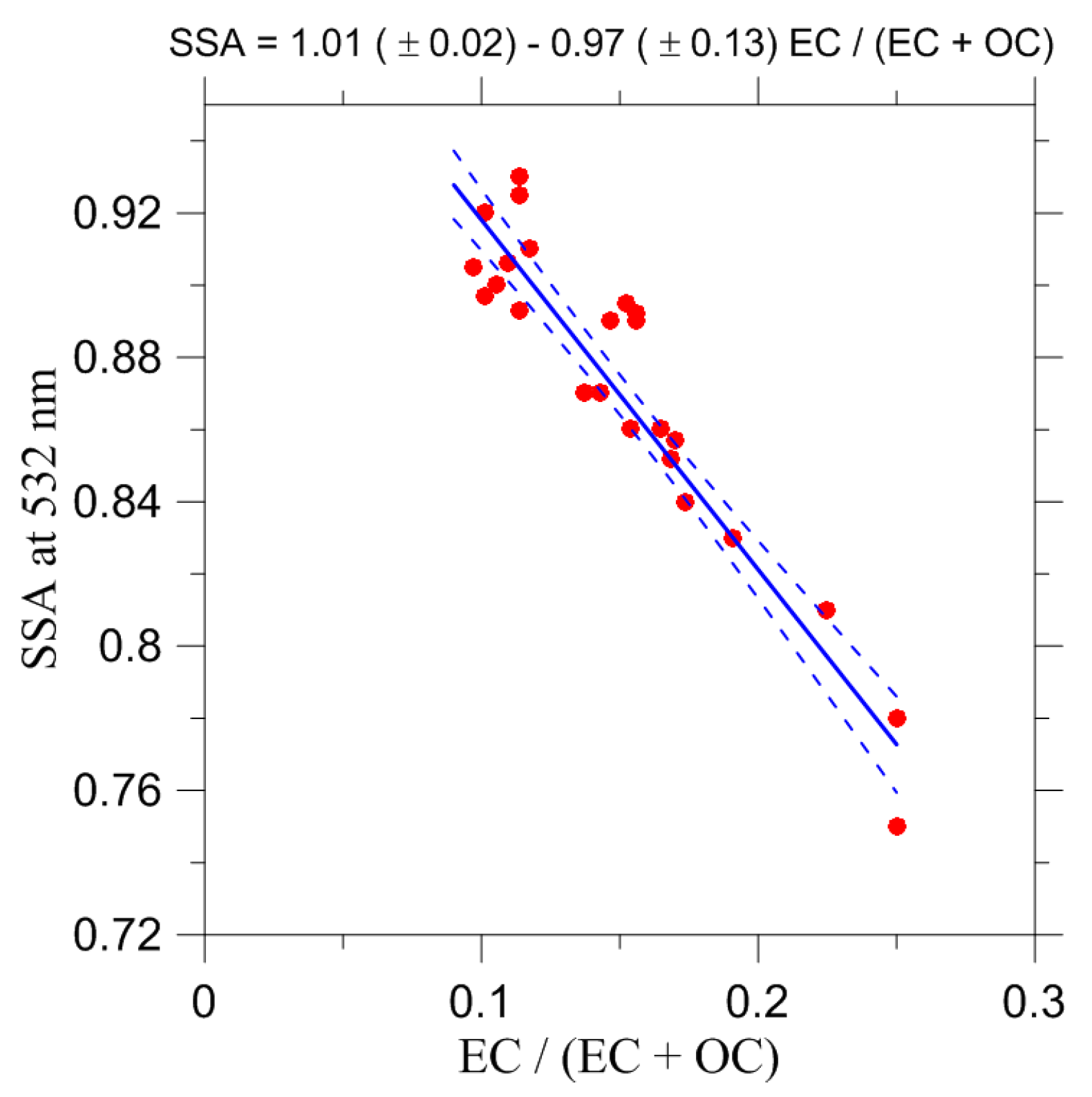
Wavelength (nm)	Slope (a)	Intercept (b)
405	−1.07 (±0.08)	0.94 (±0.007)
532	−1.06 (±0.04)	0.99 (±0.004)
660	−1.11 (±0.04)	0.99 (±0.004)

along with their uncertainties. It is noteworthy that a^λ was found to be about minus unity for all of the wavelengths considered.

The linear relationship given by Equation (2) was proven [52] to be applicable not only to fresh and dry aerosol in a controllable laboratory environment, but also to actual aging atmospheric aerosol. Specifically, SSA values predicted for the 660-nm wavelength using Equation (2) with the parameter values fitted against the FLAME-4 data were found to be in a reasonably good agreement with observations of SSA at 637 nm made during major fires in African savanna [18]. Moreover, the SSA predictions for 532 nm were found to be consistent with (although smaller than) corresponding observations of BB aerosol onboard aircraft intersecting forest fire plumes in North America [70]. To further illustrate the applicability of the linear relationship given by Equation (2) to actual atmospheric aerosol, we plotted the relationship between SSA at 532 nm and the EC/(EC + OC) ratio (see Figure 1) using the same aircraft measurements [70] and fitted a linear regression line corresponding to Equation (2). Note that following the approach used previously [52], the EC/(EC + OC) ratio was derived from the measurement data for the BC and PM_2.5 enhancement mass ratio by assuming that the OC mass fraction of the PM_2.5 was 39%. Evidently, the linear approximation fits the data shown in Figure 1 quite adequately. Additionally, it is again noteworthy that the coefficient of proportionality a^λ (see the fitting equation shown in Figure 1) was found be about minus unity.

In principle, Equation (2) could be inverted and directly used to estimate the elemental to total carbon ratio as a function of SSA as follows:

$$\frac{[EC]}{[EC]+[OC]}\cong ({\omega }_0^{\lambda }-b^{\lambda })/a^{\lambda }$$

(3)

However, it can be noticed that in the case of highly reflective BB aerosol (e.g., with SSA of 0.95 and higher), which is typically observed by AERONET in boreal regions [71], such an estimate of the elemental to total carbon ratio would be very sensitive to uncertainties in b^λ, especially at shorter wavelengths (as confirmed below in Section 3). Furthermore, in the limiting case when the EC/OC ratio approaches zero and b^λ is expected to approximate an observed value of SSA, BB aerosol absorption is likely to be mostly determined by BrC concentration, which has been shown to strongly decrease as BB aerosol ages [16]. This reasoning is confirmed by the fact that the discussed parameterization fitted to the laboratory data was previously found [52], as mentioned above, to systematically (even though not significantly) underestimate actual SSA (at 532 nm) available from the aircraft observations. Therefore, we suppose that the estimates of b^λ derived for fresh BB aerosol from the FLAME-4 data may be not always representative of actual atmospheric BB aerosol that has been exposed to aging processes (unlike smoke aerosol analyzed in FLAME-4), especially at shorter wavelengths (e.g., less than 500 nm) where the absorption of BrC typically becomes quite significant.

In contrast, we assume that the estimates of a^λ from the FLAME-4 study [52] are sufficiently robust and representative of aged aerosol observed in the AERONET stations in Siberia. This assumption is upheld by the fact that the available estimates of a^λ for fresh aerosol (see Table 2), unlike the estimates for a^λ, are practically independent (within their uncertainties) on the wavelength and thus on BrC absorption. Furthermore, there is no significant difference between the estimates of a^λ for the 532-nm wavelength, which were derived from the FLAME-4 data (see Table 2) and aircraft measurements of aging aerosol (see Figure 1). Apart from variations in BrC absorption, which can change very significantly both with the wavelength (e.g., [15]) and the BB aerosol age [16], significant deviations of a^λ from the estimates obtained for fresh and dry aerosol can potentially be caused by major morphological changes in BB aerosol particles due to aerosol aging [57]. However, as explained above (see Section 2.1.1), we tried to minimize the possibility that such changes affected the observations selected for our analysis.

Accordingly, our analysis is based on the two main assumptions: (1) the relationship between SSA and the elemental to total carbon ratio in BB aerosol is approximately linear; and (2) the optimal estimates found in the analysis of the FLAME-4 data for the parameter a^λ at the wavelengths 660 and 532 nm (a⁶⁶⁰ and a⁵³²) of the relation specified in Equation (2) are sufficiently representative (given the reported uncertainty range) of actual aging BB aerosol. In addition, following previous studies (e.g., [15]), we assume that the contribution of BrC to BB aerosol absorption at 869 nm is negligible, and so, SSA at 869 nm (ω₀⁸⁶⁹) should approach unity as the elemental carbon content approaches zero. Therefore, using Equation (2), we posit:

$$\frac{[EC]}{[EC]+[OC]}\cong ({\omega }_0^{869}-1)/{\alpha }^{869}$$

(4)

However, the value of a⁸⁶⁹ is unknown. To exclude it from the analysis, we substitute Equation (4) into Equation (2) and obtain:

$${\omega }_0^{\lambda }\cong {{\rm A}}^{\lambda }{\omega }_0^{869}+{{\rm B}}^{\lambda }$$

(5)

where,

$${{\rm A}}^{\lambda }=a^{\lambda }/a^{869},{{\rm B}}^{\lambda }=b^{\lambda }-a^{\lambda }/a^{869}$$

(6)

Values of A^λ and B^λ can be readily estimated by fitting a linear regression to the relationship between the available observations of SSA at 675 or 440 nm and SSA at 869 nm. Then, using Equation (5), Equation (3) can be re-written as follows:

$$\frac{[EC]}{[EC]+[OC]}\cong ({\omega }_0^{869}-1)A^{\lambda }/a^{\lambda }$$

(7)

or also in another form:

$$\frac{[EC]}{[OC]}\cong {\left[\frac{1}{({\omega }_0^{869}-1)A^{\lambda }/a^{\lambda }}-1\right]}^{-1}$$

(8)

Note that neither b^λ nor B^λ are used in Equations (7) and (8). In essence, we use SSA measurements at two wavelengths along with experimental estimates of the proportionality coefficient, a^λ, relating the elemental to total carbon ratio and SSA at a given wavelength λ, to calibrate the unknown value of a⁸⁶⁹.

Our best (the “base case” or “Case 1”) estimates of the EC to OC ratio are based on using the AERONET SSA observations at 675 and 869 nm along with the estimate of a⁶⁷⁵, which was obtained from the power-law extrapolation from available values of the absolute values of a⁶⁶⁰ and a⁵³² (see Table 2). For comparison, we consider three other cases listed in

Table 3. Distinctive features of the different cases of estimation of the EC/OC ratio using the AERONET observations.

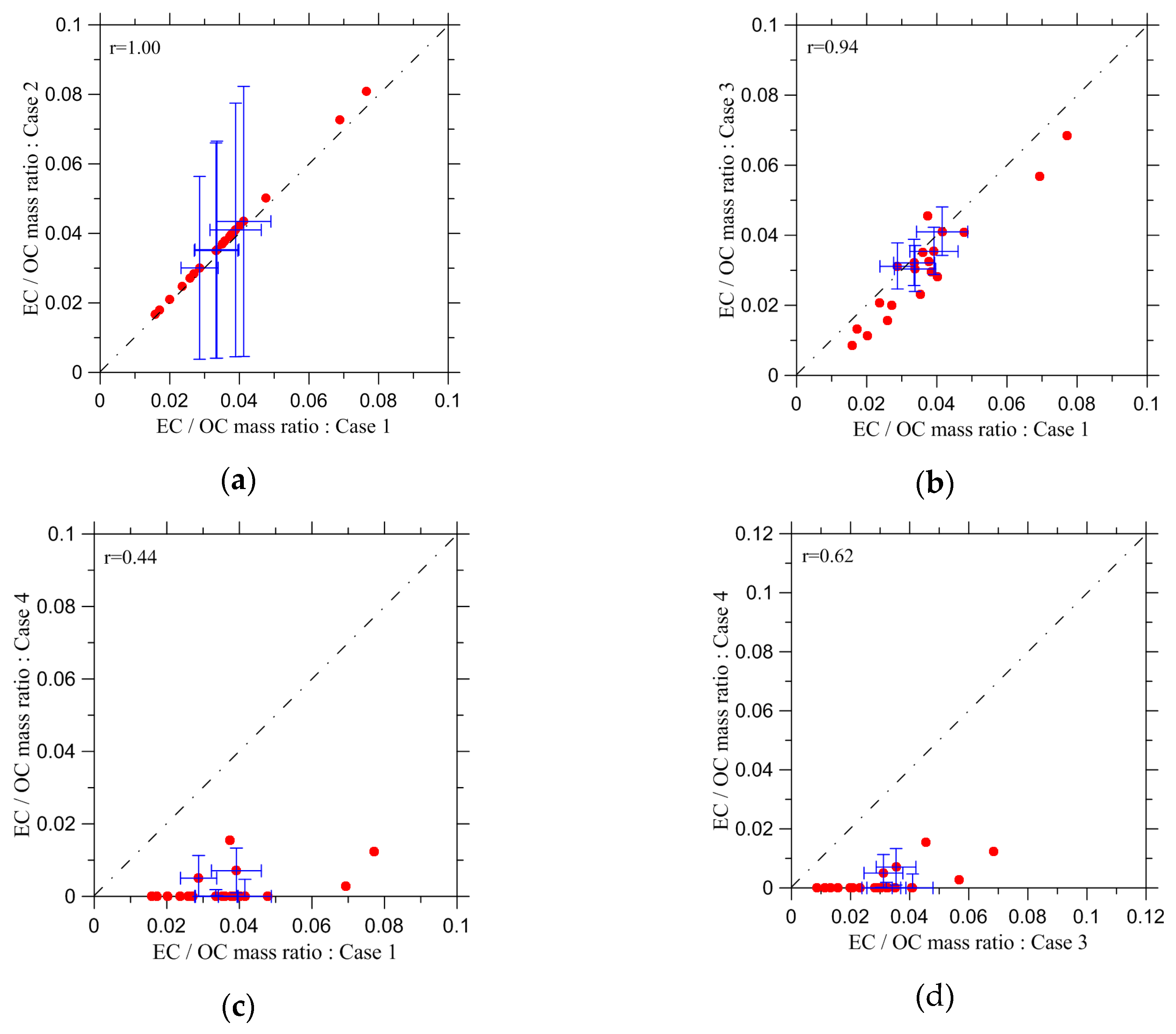
Estimation Cases	Distinctive Features of Estimation Procedures
Case 1	The estimates are obtained using Equation (8) and SSA observations at 675 nm
Case 2	The same as Case 1, but using SSA observations at 440 nm
Case 3	The estimates are obtained using the available parameterization [52] for SSA at 660 nm (see Equation (1) and Table 2)
Case 4	The same as Case 3, but using the similar parameterization for SSA at 405 nm

. Specifically, the Case 2 estimate is also obtained with Equation (8), but using SSA observations at 440 nm along with the corresponding estimate of a⁴⁴⁰ derived by the power-law interpolation between the experimental estimates of a⁴⁰⁵ and a⁵³². The Cases 3 and 4 are based on a direct application of the available linear approximations (see Equation (3) and Table 2) from the FLAME-4 study [52] to the SSA values obtained correspondingly for the 660- and 405-nm wavelengths by interpolation or extrapolation from the AERONET SSA observations at the 675- and 440-nm wavelengths. In other words, Cases 3 and 4 involve not only the available estimates of a^λ (as in Cases 1 and 2), but the estimates of b^λ, as well. Along with the different observation-based estimates of the EC/OC ratio, we consider predictions of the EC/OC ratio from the 3D model simulations (see Section 2.1.2). The model estimates are calculated as the ratio of the column mass densities of EC and OC in primary and secondary aerosol originating from fire emissions.

Note that all of the estimates for a^λ, b^λ, A^λ and B^λ employed in our analysis are obtained using the orthogonal distance regression (ODR). Unlike a simple linear regression model, which is based on the assumption that an explanatory variable is not affected by errors and which minimizes the distance between the dependent variable and the fitting line only in the vertical direction, the ODR method allows for observation errors in both the explanatory and dependent variables and minimizes the orthogonal distances between each data point and the regression line. Therefore, the use of the ODR method ensures that the linear fits analyzed below are sufficiently symmetric with respect to the choice of the explanatory and dependent variables, and so, the corresponding linear approximations can be inverted as suggested by Equations (3) and (7).

As noted in the Introduction, one of the main goals of our analysis was to create a robust parameterization that would allow one to estimate the EC/OC ratio in BB aerosol by using available satellite observations, such as the retrievals of the absorption AOD at 388 nm (AAOD³⁸⁸) from the OMI measurements [46] and the retrievals of the extinction AOD at 550 nm (AOD⁵⁵⁰) from the MODIS measurements [53]. To this end, we consider the ratio of AAOD³⁸⁸ to AOD⁵⁵⁰ as a function of the EC/(EC + OC) ratio estimated as described above for the Case 1. We expect that inasmuch as there is a regular relationship between the EC/(EC + OC) ratio and SSA at 440 nm, there should also be a similar relationship between the EC/(EC + OC) and AAOD³⁸⁸/AOD⁵⁵⁰ ratios.

Indeed, SSA at 440 nm (ω₀⁴⁴⁰) can, by definition, be expressed through the ratio of AAOD and AOD at 440 nm (AAOD⁴⁴⁰ and AOD⁴⁴⁰):

$${\omega }_0^{440}=1-\frac{AAO{D}^{440}}{AO{D}^{440}}$$

(9)

Both AAOD⁴⁴⁰ and AOD⁴⁴⁰ can be extrapolated to the 388-nm and 550-nm wavelengths, respectively, using the corresponding Ångström exponents, α_a and α_e, which, in turn, can be evaluated using the AERONET observations at two different wavelengths.

$${\alpha }_a=-\frac{\log (AAO{D}^{440}/AAO{D}^{675})}{\log (440/675)},{\alpha }_e=-\frac{\log (AO{D}^{440}/AO{D}^{500})}{\log (440/500)}$$

(10)

The uncertainties (confidence intervals) for any coefficients of linear regressions built in this study were evaluated using a Monte Carlo procedure based on one of the standard bootstrapping techniques [72]. The procedure comprised 5000 iterations involving random sampling of N (20, in our case) data points from the original dataset (including the same number, N, of data points). The sampled data were then used in each of the iterations to obtain perturbed estimates of a given parameter (e.g., the slope of the linear regression in Equation (5) or the mean of the estimates for individual observations) in the same way as the original data were used to obtain a corresponding optimal estimate. The underlying assumption in this procedure is that the errors of individual SSA observations are statistically independent. Wherever an estimation involved uncertainties in input parameters (as, e.g., in the case of the estimation given by Equation (8)), such uncertainties were taken into account by randomly perturbing the corresponding parameter values (within the range of their uncertainties; see Table 2) in each iteration of the same Monte Carlo procedure. The spread of estimates from different iterations was used to evaluate the confidence intervals for a corresponding optimal estimate. For definiteness, the confidence intervals of all estimates reported below (including estimates of regression coefficients) are given in terms of the 90th percentile.

3. Results

Figure 2 and Figure 3 characterize the impact of open biomass burning in Siberia on AOD observed at the two AERONET sites (indicated in Figure 2) that provided the data for this study. Specifically, Figure 2 shows the spatial averages of AOD at 500 nm according to the CHIMERE simulations made with and without fire emissions for the Siberian model domain; the averages were calculated over the selection of the simulated AOD values corresponding in time to the AERONET retrievals selected for our analysis (see Section 2.1.1). Figure 3 shows the time series of the simulated AOD values along with the observed AOD values for our selection of the AERONET retrievals. Additionally, Figure 3 also illustrates the selection of SSA observations with respect to relative humidity (see Section 2.1.1 and Table 1).

Evidently, the simulation results presented in the both figures indicate that fires had a major impact on AOD at the locations considered and provided a predominant component of observed aerosol on many days in summer 2012. Furthermore, our simulations are supportive of the validity of the selection criterion (requiring that AOD at 500 nm exceeds 0.5; see Table 1), which was used as an indicator of a predominant contribution of biomass burning to aerosol observed at the AERONET sites considered. Specifically, according to our simulations shown in Figure 3, the contribution of BB aerosol resulted in large enhancements of AOD observed in the selected episodes with respect to the background AOD (by more than a factor of six on average and by at least a factor of three in almost all of the selected individual episodes). In addition, the comparison of AAOD observations with the background AAOD predicted by the model (the corresponding data are not shown) indicated even larger enhancements, by factors of eleven and eight on average, in AAOD at 675 and 440 nm, respectively: this result is not surprising taking into account that, according to our simulations, a dominant mass fraction of background aerosol at the both sites is constituted by biogenic SOA, which is very weakly absorptive [73].

Figure 4 shows the relations between the AERONET observations of SSA at 675 nm and 440 nm and those at 869 nm. The relations were fitted with the linear model given by Equation (5). Evidently, the SSA values for the 869-nm wavelength very strongly correlate with those for the 675-nm wavelength (R = 0.98), and the relation between them is indeed practically linear. These observations confirm our reasoning behind Equation (5) explained in Section 2.2. The correlation of SSA at 869 nm with SSA at 440 nm is much weaker, but it is still rather considerable (R = 0.62), and there is no visible evidence that the corresponding relationship is strongly nonlinear. It is noteworthy that the slopes of the linear fits (A⁶⁷⁵ and A⁴⁴⁰) are close to unity, being statistically different from zero. In view of the relation given by Equation (6) and the available estimates for a⁶⁷⁵ and a⁴⁴⁰ (which are both near minus unity), this fact indicates that a⁸⁶⁹ is also close to minus unity. In contrast, the intercepts, B⁶⁷⁵ and B⁴⁴⁰ are not statistically different from zero.

The estimates of the EC/OC ratios for the different cases specified above (see Table 3) are presented and compared in Figure 5. In addition, the mean values and their confidence intervals for the different types of estimates are listed in

Table 4. Average values of the EC/OC ratio estimates derived from the AERONET observations according to different estimation cases along with the corresponding value predicted by simulations with the CHIMERE model. The numbers in parentheses indicate the 90% confidence intervals for the average estimates based on observations. The uncertainty of the model predictions has not been evaluated in this study.

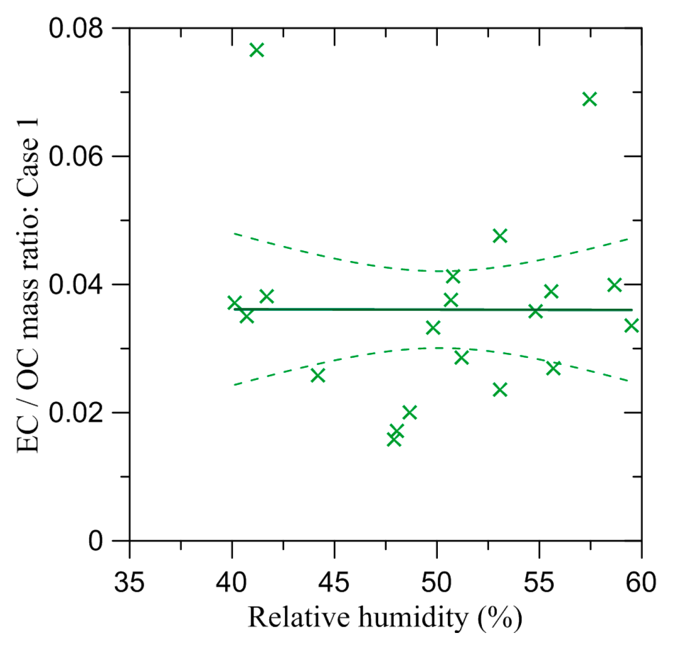
Estimation Case	Average Value of the EC/OC Ratio
Case 1	0.036 (±0.009)
Case 2	0.038 (±0.035)
Case 3	0.031 (±0.009)
Case 4	0.002 (±0.011)
CHIMERE	0.061

, which also reports the mean value for the corresponding model predictions of the EC/OC ratio. Values of our best (Case 1) estimates range from 0.015–0.077, with the mean value of 0.036. It is useful to note that this value is in a very good agreement with the recently reported [74] value of EC/OC enhancement ratio (0.038) evaluated for BB aerosol in Siberia using the long-term in situ measurements of carbonaceous aerosol at the Zotino tall tower observatory (ZOTTO). Taking into account the uncertainties of the fits involved in the estimation procedures, one can see that the base case estimates almost perfectly agree with the Case 2 estimates (see Figure 5a). This finding upholds the assumption about the linear dependence of SSA (within the range of wavelengths considered in this study) on the EC/(EC + OC) ratio. Furthermore, it can be regarded as evidence that the AERONET observations are consistent with the estimate of a⁴⁴⁰ based on the FLAME-4 analysis.

The base case estimates are also consistent with estimates for the Case 3, although the Case 3 estimates are slightly, but systematically smaller than the Case 1 estimates. This consistency is not surprising, taking into account that the BrC absorption (that, as noted above, might be the main reason for a possible inconsistency of the b^λ estimates derived from the FLAME-4 data with the AERONET observations) is likely to be small at the 660nm wavelength (e.g., [15]). This finding indicates that the SSA parameterization derived from the FLAME-4 data for the 660-nm wavelength is consistent (although not ideally) with the AERONET observations of BB aerosol in Siberia.

In contrast, there are major inconsistencies between the Case 1 and 4 estimates, as well as between the Case 3 and 4 estimates. In fact, Equation (2) with the parameters fitted with the FLAME-4 data for the 405-nm wavelength (see Table 2) predicts mostly negative (that is, unphysical) values for the EC/OC ratio; such values are replaced in Figure 5 by zeros. These inconsistencies indicate that the SSA parameterization derived from the FLAME-4 data for the 405-nm wavelength is not directly applicable to the BB burning aerosol observations in Siberia. Presumably, the discrepancy between the Case 4 estimates and the other estimates is mainly due to a strong effect of BB aerosol aging processes on the short-wave light absorption by brown carbon.

Our estimates of the EC/OC ratio for the base case are compared with the corresponding predictions by CHIMERE in Figure 6. Obviously, the model tends to overestimate the EC/OC ratio, even though the differences between individual estimates can, in many instances, be explained by the uncertainty of the AERONET SSA retrievals. Specifically, the model predictions are larger than the observation-based estimates in 18 from 20 episodes considered, with the simulated mean value (0.061) being a factor of 1.7 larger than the mean value for our estimates. The modeled estimates for the EC/OC ratio are also characterized by much smaller variability than the observation-based estimates. Furthermore, it is evident (see Figure 6) that the variability of the observation-based estimates cannot be explained by the model. However, we cannot claim that the variability of our estimates is representative of the actual variability of the EC/OC ratio, as our estimates are subject to a potential large uncertainty in the SSA retrievals. The fact that the model predicted larger values of the EC/OC ratio in BB aerosol than the EC/OC ratio (0.052) assumed for forest fire emissions is indicative of a considerable contribution of grass (and/or agricultural) fires. However, according to our simulations, the forest fires are evidently a predominant source of BB aerosol at the sites considered, since otherwise the simulated EC/OC ratio in the aerosol particles would be much larger (taking into account that the EC/OC ratios assumed for the grass and agricultural fires were 0.14 and 0.32, respectively, while the contribution of SOA to the OC columns was always less than 15%).

The observation-based and model estimates of the EC/OC ratio for Case 1 are considered as a function the photochemical age of BB aerosol in Figure 7. The estimates derived from the AERONET observations demonstrate a weak positive association (at the edge of statistical significance) with the photochemical age. The modeled estimates are practically independent of the photochemical age. The absence of large systematic changes in the EC/OC ratio with changes of the photochemical age can be considered as additional evidence that our estimates are sufficiently robust with respect to BB aerosol aging.

Theoretically, an increase in the EC/OC ratio may be due to evaporation of organic matter (OM) upon dilution of BB plumes, as well as due to fragmentation processes involving semi-volatile organic compounds [75]. There is observational evidence (e.g., [76]) confirming that the OM enhancement ratio (that is, the ratio of mass concentration of OM in BB aerosol to that of the BB fraction of a long-lived tracer, such as, e.g., CO) can indeed decrease as aerosol ages, although there is also evidence that the OM enhancement ratio can increase with the age (e.g., [18,19]). Using satellite observations of AOD over Siberia [20], a significant increase (followed by a decrease) of the OM enhancement ratio during about the first 15 hours of BB aerosol evolution was detected in dense BB plumes selected as the high (70th and higher) percentiles of the observed and modeled CO columns. However, the amount of data available for this study was insufficient for any conclusions regarding the evolution of the EC/OC ratio in BB aerosol aged less than 15 h. Furthermore, this study did not involve pre-selection of the most dense plumes (because of an insufficient amount of available data), except for the application of a general criterion aimed to identify BB aerosol in AERONET observations.

Note that since the large differences between the Case 1 and Case 4 estimates are likely due to the effects of photochemical aging (as discussed above), the Case 4 estimates could be expected to be more strongly dependent on the photochemical age than the Case 1 estimates. However, the available data allowed us to obtain physically meaningful Case 4 estimates of the EC/OC ratio only for five episodes (see Figure 5), and so, the corresponding statistical analysis was not feasible with a such a small amount of data.

It was shown earlier [20] that BB aerosol simulations using the “standard” representation (as in this study) of organic aerosol processes in the CHIMERE model predict a slight increase of the OM enhancement ratio as a result of SOA formation. Accordingly, it could be expected that the EC/OC ratio predicted by the model should be a slowly decreasing function of the BB aerosol photochemical age. Taking into account the scatter of the model data presented in Figure 7, the simulated values of the EC/OC ratio are not inconsistent with this expectation.

Figure 8 examines a potential impact of ambient relative humidity (RH) in the BB aerosol columns on our estimates. The absence of a significant dependence of the EC/OC ratio on RH confirms that the SSA observations selected for our analysis (using a criterion requiring that RH should be less 60%) and ensuing estimates are not systematically affected by RH variations in the considered range of its values.

Finally, the AAOD³⁸⁸/AOD⁵⁵⁰ ratio is plotted as a function of the EC/(EC + OC) ratio in Figure 9. The variables are positively correlated (R = 0.63), although there is a considerable scatter of the data. The linear fit (obtained with the ODR method) to the relationship between the AAOD³⁸⁸/AOD⁵⁵⁰ and EC/(EC + OC) ratios is given by the following equation:

$$\frac{AAO{D}^{388}}{AO{D}^{550}}=2.05(\pm 0.86)\frac{[EC]}{[EC]+[OC]}+0.014(\pm 0.028).$$

(11)

Importantly, the slope of the linear fit is estimated to be a positive value, which is statistically different from zero. Note that the relation given by Equation (11) can be easily rewritten using the EC/OC ratio instead of the EC/(EC + OC) ratio, as is done above in the case of Equation (7). Overall, the results shown in Figure 9 indicate that if typical values of the AAOD³⁸⁸/AOD⁵⁵⁰ ratio retrieved from satellite measurements fall into the range of values representative of the AERONET observations analyzed in this study, the mean value of the EC/OC ratio can be constrained within the relative uncertainty of about 50%, which is much lower than probable uncertainties of the ratio of the EC and OC emission factors in fire emission inventories.

4. Conclusions

In this paper, we examined feasibility of using observations of aerosol optical properties at AERONET sites to estimate the EC/OC mass ratio in BB aerosol in Siberia and to create a parameterization relating the EC/OC ratio with the ratio of AAOD and AOD retrievals from available satellite observations. Our method for estimation of the EC/OC ratio is based on the recent robust findings from the FLAME-4 study [52] of the chemical composition and optical properties of aerosol emitted from laboratory combustion of a range of wildland fuels. Specifically, consistent with the experimental findings, we presumed that SSA of BB aerosol particles at the submicrometer wavelengths depends linearly on the elemental to total carbon ratio, EC/(EC + OC), with the coefficient of proportionality of about minus unity. Using the retrievals at the 869-, 675- and 440-nm wavelengths from the measurements at the “Tomsk-22” and “Yakutsk” AERONET sites in summer 2012, we obtained estimates for the EC/OC ratio in BB aerosol in Siberia and examined the consistency of the parameterizations derived earlier [52] from the FLAME-4 data for SSA at the 660- and 405-nm wavelengths. Simulations performed with the CHIMERE chemistry transport model were employed to ensure that BB aerosol was a predominant aerosol type in the observed episodes selected for our analysis, as well as to estimate the photochemical age of BB aerosol in those episodes.

Our estimates of the EC/OC mass ratio range from 0.015–0.077, with the mean value of 0.036 (±0.009). The estimated mean value of the EC/OC ratio is found to be significantly smaller than the corresponding value (0.06) predicted by the BB aerosol simulations based on the emission factors specified in the GFED4 emission inventory, but in a very good agreement with the recently reported [74] value of the EC/OC enhancement ratio (0.038) evaluated in long-term in situ measurements of carbonaceous aerosol at the Zotino tall tower observatory. Our estimates indicate that the EC/OC mass ratio tends to increase with the photochemical age of BB aerosol, although the statistical significance of the tendency is rather low. No association is found between the EC/OC ratio and ambient relative humidity (RH) in the range of RH values less than 60%; observations corresponding to higher levels of RH were not considered in this study.

The EC/OC ratio estimates derived from the AERONET SSA observations with our method using the combination of observations at 869-nm and 675-nm wavelengths are found to be consistent with the corresponding estimates derived in the same way, but using the combination of observations at 869-nm and 440-nm wavelengths, although the estimates in the latter case proved to be much more uncertain. In contrast, there are significant discrepancies between the estimates obtained using the AERONET data with the original FLAME-4 parameterizations for SSA of fresh BB aerosol at the 660- and 405-nm wavelengths. Specifically, the parameterization for 405 nm is found to strongly underestimate the EC/OC ratio. We argue that the underestimation may be due to a decrease of BrC absorption by atmospheric aging of BB aerosol. Therefore, possible future applications of parameterizations for the EC/OC ratio, which are based on SSA measurements of fresh BB aerosol at wavelengths where the BrC absorption may be significant, to the actual aging BB aerosol require special precautions.

Finally, we proposed a parameterization relating the EC/OC ratio and the ratio of the absorption AOD to the extinction AOD at 388- and 550-nm wavelengths, respectively. Since the corresponding absorption and extinction AOD data are presently available as retrievals from the OMI and MODIS satellite measurements, this parameterization may be helpful for constraining EC (or BC) emissions from wildfires in Siberia. The applicability of our parameterization to other regions affected by intense biomass burning requires further research.

References

- Intergovermental Panel on Climate Change. Climate Change 2013: The Physical Science Basis; Summary for Policymakers; Cambridge University Press: Cambridge, UK, 2013. [Google Scholar]
- Ten Hoeve, J.E.; Jacobson, M.Z.; Remer, L. Comparing results from a physical model with satellite and in situ observations to determine whether biomass burning aerosols over the Amazon brighten or burn off clouds. J. Geophys. Res. 2012, 117, D08203. [Google Scholar] [CrossRef]
- Jacobson, M.Z. Effects of biomass burning on climate, accounting for heat and moisture fluxes, black and brown carbon, and cloud absorption effects. J. Geophys. Res. Atmos. 2014, 119, 980–9002. [Google Scholar] [CrossRef]
- Konovalov, I.B.; Beekmann, M.; Kuznetsova, I.N.; Yurova, A.; Zvyagintsev, A.M. Atmospheric impacts of the 2010 Russian wildfires: Integrating modelling and measurements of an extreme air pollution episode in the Moscow region. Atmos. Chem. Phys. 2011, 11, 10031–10056. [Google Scholar] [CrossRef]
- Strand, T.M.; Larkin, N.; Craig, K.J.; Raffuse, S.; Sullivan, D.; Solomon, R.; Rorig, M.; Wheeler, N.; Pryden, D. Analyses of BlueSky Gateway PM2.5 predictions during the 2007 southern and 2008 northern California fires. J. Geophys. Res. 2012, 117, D17301. [Google Scholar] [CrossRef]
- Navarro, K.M.; Cisneros, R.; O’Neill, S.M.; Schweizer, D.; Larkin, N.K.; Balmes, J.R. Air-Quality Impacts and Intake Fraction of PM2.5 during the 2013 Rim Megafire. Environ. Sci. Technol. 2016, 50, 11965–11973. [Google Scholar] [CrossRef] [PubMed]
- Bond, T.C.; Doherty, S.J.; Fahey, D.W.; Forster, P.M.; Berntsen, T.; DeAngelo, B.J.; Flanner, M.G.; Ghan, S.; Kärcher, B.; Koch, D.; et al. Bounding the role of black carbon in the climate system: A scientific assessment. J. Geophys. Res. Atmos. 2013, 118, 5380–5552. [Google Scholar] [CrossRef]
- Myhre, G.; Samset, B.H.; Schulz, M.; Balkanski, Y.; Bauer, S.; Berntsen, T.K.; Bian, H.; Bellouin, N.; Chin, T.; Diehl, T.; et al. Radiative forcing of the direct aerosol effect from AeroCom Phase II simulations. Atmos. Chem. Phys. 2013, 13, 1853–1877. [Google Scholar] [CrossRef]
- Saleh, R.; Robinson, E.S.; Tkacik, D.S.; Ahern, A.T.; Liu, S.; Aiken, A.C.; Sullivan, R.C.; Presto, A.A.; Dubey, M.K.; Yokelson, R.J.; et al. Brownness of organics in aerosols from biomass burning linked to their black carbon content. Nature Geosci. 2014, 7, 647–650. [Google Scholar] [CrossRef]
- Lu, Z.; Streets, D.G.; Winijkul, E.; Yan, F.; Chen, Y.; Bond, T.C.; Feng, Y.; Dubey, M.K.; Liu, S.; Pinto, J.P.; et al. Light absorption properties and radiative effects of primary organic aerosol emissions. Environ. Sci. Technol. 2015, 49, 4868–4877. [Google Scholar] [CrossRef] [PubMed]
- Wang, X.; Heald, C.L.; Sedlacek, A.J.; de Sá, S.S.; Martin, S.T.; Alexander, M.L.; Watson, T.B.; Aiken, A.C.; Springston, S.R.; Artaxo, P. Deriving brown carbon from multiwavelength absorption measurements: Method and application to AERONET and Aethalometer observations. Atmos. Chem. Phys. 2016, 16, 12733–12752. [Google Scholar] [CrossRef]
- Pokhrel, R.P.; Beamesderfer, E.R.; Wagner, N.L.; Langridge, J.M.; Lack, D.A.; Jayarathne, T.; Stone, E.A.; Stockwell, C.E.; Yokelson, R.J.; Murphy, S.M. Relative importance of black carbon, brown carbon, and absorption enhancement from clear coatings in biomass burning emissions. Atmos. Chem. Phys. 2017, 17, 5063–5078. [Google Scholar] [CrossRef]
- Chung, C.E.; Ramanathan, V.; Decremer, D. Observationally constrained estimates of carbonaceous aerosol radiative forcing. Proc. Natl. Acad. Sci. USA 2012, 109, 11624–11629. [Google Scholar] [CrossRef] [PubMed]
- Kirchstetter, T.W.; Thatcher, T.L. Contribution of organic carbon to wood smoke particulate matter absorption of solar radiation. Atmos. Chem. Phys. 2012, 12, 6067–6072. [Google Scholar] [CrossRef]
- Bahadur, R.; Praveen, P.S.; Xu, Y.; Ramanathan, V. Solar absorption by elemental and brown carbon determined from spectral observations. Proc. Natl. Acad. Sci. USA 2012, 109, 17366–17371. [Google Scholar] [CrossRef] [PubMed]
- Forrister, H.; Liu, J.; Scheuer, E.; Dibb, J.; Ziemba, L.; Thornhill, K.L.; Anderson, B.; Diskin, G.; Perring, A.E.; Schwarz, J.P.; et al. Evolution of brown carbon in wildfire plumes. Geophys. Res. Lett. 2015, 42, 4623–4630. [Google Scholar] [CrossRef]
- Akagi, S.K.; Craven, J.S.; Taylor, J.W.; McMeeking, G.R.; Yokelson, R.J.; Burling, I.R.; Urbanski, S.P.; Wold, C.E.; Seinfeld, J.H.; Coe, H.; et al. Evolution of trace gases and particles emitted by a chaparral fire in California. Atmos. Chem. Phys. 2012, 12, 1397–1421. [Google Scholar] [CrossRef]
- Vakkari, V.; Kerminen, V.M.; Beukes, J.P.; Tiitta, P.; van Zyl, P.G.; Josipovic, M.; Venter, A.D.; Jaars, K.; Worsnop, D.R.; Kulmala, M.; et al. Rapid Changes in biomass burning aerosols by atmospheric oxidation. Geophys. Res. Lett. 2014, 41, 2644–2651. [Google Scholar] [CrossRef]
- Konovalov, I.B.; Beekmann, M.; Berezin, E.V.; Petetin, H.; Mielonen, T.; Kuznetsova, I.N.; Andreae, M.O. The role of semi-volatile organic compounds in the mesoscale evolution of biomass burning aerosol: A modeling case study of the 2010 mega-fire event in Russia. Atmos. Chem. Phys. 2015, 15, 13269–13297. [Google Scholar] [CrossRef]
- Konovalov, I.B.; Beekmann, M.; Berezin, E.V.; Formenti, P.; Andreae, M.O. Probing into the aging dynamics of biomass burning aerosol by using satellite measurements of aerosol optical depth and carbon monoxide. Atmos. Chem. Phys. 2017, 17, 4513–4537. [Google Scholar] [CrossRef]
- Andreae, M.O.; Gelencsér, A. Black carbon or brown carbon? The nature of light-absorbing carbonaceous aerosols. Atmos. Chem. Phys. 2006, 6, 3131–3148. [Google Scholar] [CrossRef]
- Van der Werf, G.R.; Randerson, J.T.; Giglio, L.; Collatz, G.J.; Mu, M.; Kasibhatla, P.S.; Morton, D.C.; DeFries, R.S.; Jin, Y.; van Leeuwen, T.T. Global fire emissions and the contribution of deforestation, savanna, forest, agricultural, and peat fires (1997–2009). Atmos. Chem. Phys. 2010, 10, 11707–11735. [Google Scholar] [CrossRef]
- Wiedinmyer, C.; Akagi, S.K.; Yokelson, R.J.; Emmons, L.K.; Al-Saadi, J.A.; Orlando, J.J.; Soja, A.J. The Fire INventory from NCAR (FINN): A high resolution global model to estimate the emissions from open burning. Geosci. Model Dev. 2011, 4, 625–641. [Google Scholar] [CrossRef]
- Kaiser, J.W.; Flemming, J.; Schultz, M.G.; Suttie, M.; Wooster, M.J. The MACC global fire assimilation system: first emission products (GFASv0). ECMWF Tech. Memo. 2009, 596, 1–16. [Google Scholar]
- Akagi, S.K.; Yokelson, R.J.; Wiedinmyer, C.; Alvarado, M.J.; Reid, J.S.; Karl, T.; Crounse, J.D.; Wennberg, P.O. Emission factors for open and domestic biomass burning for use in atmospheric models. Atmos. Chem. Phys. 2011, 11, 4039–4072. [Google Scholar] [CrossRef]
- Andreae, M.O.; Merlet, P. Emission of trace gases and aerosols from biomass burning. Glob. Biogeochem. Cycles 2001, 15, 955–966. [Google Scholar] [CrossRef]
- Andreae, M.O.; (Max Planck Institute for Chemistry, Mainz, Germany). Biomass burning emission factors. Personal communication, 2015. [Google Scholar]
- Schmidt, T.L.; Raile, G.K. Sustainability of Siberia and Far East Russia’s Forest Resource. J. Sustain. For. 2000, 11, 1–21. [Google Scholar] [CrossRef]
- Sutton, W. Siberia has a very large forest resource but…. N. Z. J. For. 2013, 58, 16–19. [Google Scholar]
- Konovalov, I.B.; Berezin, E.V.; Ciais, P.; Broquet, G.; Beekmann, M.; Hadji-Lazaro, J.; Clerbaux, C.; Andreae, M.O.; Kaiser, J.W.; Schulze, E.-D. Constraining CO2 emissions from open biomass burning by satellite observations of co-emitted species: A method and its application to wildfires in Siberia. Atmos. Chem. Phys. 2014, 14, 10383–10410. [Google Scholar] [CrossRef]
- Ikeda, K.; Tanimoto, H. Exceedances of air quality standard level of PM2.5 in Japan caused by Siberian wildfires. Environ. Res. Lett. 2015, 10, 105001. [Google Scholar] [CrossRef]
- Jung, J.; Lyu, Y.; Lee, M.; Hwang, T.; Lee, S.; Oh, S. Impact of Siberian forest fires on the atmosphere over the Korean Peninsula during summer 2014. Atmos. Chem. Phys. 2016, 16, 6757–6770. [Google Scholar] [CrossRef]
- Laing, J.R.; Jaffe, D.A.; Hee, J.R. Physical and optical properties of aged biomass burning aerosol from wildfires in Siberia and the Western USA at the Mt. Bachelor Observatory. Atmos. Chem. Phys. 2016, 16, 15185–15197. [Google Scholar] [CrossRef]
- Evangeliou, N.; Balkanski, Y.; Hao, W.M.; Petkov, A.; Silverstein, R.P.; Corley, R.; Nordgren, B.L.; Urbanski, S.P.; Eckhardt, S.; Stohl, A.; et al. Wildfires in northern Eurasia affect the budget of black carbon in the Arctic—A 12-year retrospective synopsis (2002–2013). Atmos. Chem. Phys. 2016, 16, 7587–7604. [Google Scholar] [CrossRef]
- Arctic Report Card. Richter-Menge, J.; Overland, E.; Mathis, J.T. (Eds.) 2016. Available online: http://www.arctic.noaa.gov/Report-Card (accessed on 15 May 2017).
- Soja, A.J.; Cofer, W.R.; Shugart, H.H.; Sukhinin, A.I.; Stackhouse, P.W., Jr.; McRae, D.J.; Conard, S.G. Estimating fire emissions and disparities in boreal Siberia (1998–2002). J. Geophys. Res. 2004, 109, D14S06. [Google Scholar] [CrossRef]
- Randerson, J.T.; Liu, H.; Flanner, M.G.; Chambers, S.D.; Jin, Y.; Hess, P.G.; Pfister, G.; Mack, M.C.; Treseder, K.K.; Welp, L.R.; et al. The impact of boreal forest fire on climate warming. Science 2006, 314, 1130–1132. [Google Scholar] [CrossRef] [PubMed]
- Balzter, H.; Gerard, F.; Weedon, G.; Grey, W.; Combal, B.; Bartholome, E.; Bartalev, S.; Los, S. Coupling of vegetation growing season anomalies with hemispheric and regional scale climate patterns in Central and East Siberia. J. Clim. 2007, 20, 3713–3729. [Google Scholar] [CrossRef]
- Holben, B.N.; Eck, T.F.; Slutsker, I.; Tanré, D.; Buis, J.P.; Setzer, A.; Vermote, E.; Reagan, J.A.; Kaufman, Y.J.; Nakajima, T.; et al. AERONET—A federated instrument network and data archive for aerosol characterization. Remote Sens. Environ. 1998, 66, 1–16. [Google Scholar] [CrossRef]
- Dubovik, O.; King, M.D. A flexible inversion algorithm for retrieval of aerosol optical properties from Sun and sky radiance measurements. J. Geophys. Res. Atmos. 2000, 105, 20673–20696. [Google Scholar] [CrossRef]
- Sato, M.; Hansen, J.; Kock, D.; Lacis, A.; Ruedy, R.; Dubovik, O.; Holben, B.; Chin, M.; Novakov, T. Global atmospheric black carbon inferred from AERONET. Proc. Natl. Acad. Sci. USA 2003, 100, 6319–6324. [Google Scholar] [CrossRef] [PubMed]
- Koch, D.; Schulz, M.; Kinne, S.; McNaughton, C.; Spackman, J.R.; Balkanski, Y.; Bauer, S.; Berntsen, T.; Bond, T.C.; Boucher, O.; et al. Evaluation of black carbon estimations in global aerosol models. Atmos. Chem. Phys. 2009, 9, 9001–9026. [Google Scholar] [CrossRef]
- Huang, K.; Fu, J.S.; Prikhodko, V.Y.; Storey, J.M.; Romanov, A.; Hodson, E.L.; Cresko, J.; Morozova, I.; Ignatieva, Y.; Cabaniss, J. Russian anthropogenic black carbon: Emission reconstruction and Arctic black carbon simulation. J. Geophys. Res. Atmos. 2015, 120, 11306–11333. [Google Scholar] [CrossRef]
- Pan, X.; Chin, M.; Gautam, R.; Bian, H.; Kim, D.; Colarco, P.R.; Diehl, T.L.; Takemura, T.; Pozzoli, L.; Tsigaridis, K.; et al. A multi-model evaluation of aerosols over South Asia: common problems and possible causes. Atmos. Chem. Phys. 2015, 15, 5903–5928. [Google Scholar] [CrossRef]
- Ocko, I.B.; Ginoux, P.A. Comparing multiple model-derived aerosol optical properties to spatially collocated ground-based and satellite measurements. Atmos. Chem. Phys. 2017, 17, 4451–4475. [Google Scholar] [CrossRef]
- Torres, O.; Tanskanen, A.; Veihelmann, B.; Ahn, C.; Braak, R.; Bhartia, P.K.; Veefkind, P.; Levelt, P. Aerosols and surface UV products from Ozone Monitoring Instrument observations: An overview. J. Geophys. Res. 2007, 112, D24S47. [Google Scholar] [CrossRef]
- Zhang, L.; Henze, D.K.; Grell, G.A.; Carmichael, G.R.; Bousserez, N.; Zhang, Q.; Torres, O.; Ahn, C.; Lu, Z.; Cao, J.; et al. Constraining black carbon aerosol over Asia using OMI aerosol absorption optical depth and the adjoint of GEOS-Chem. Atmos. Chem. Phys. 2015, 15, 10281–10308. [Google Scholar] [CrossRef]
- Curci, G.; Hogrefe, C.; Bianconi, R.U.; Balzarini, A.; Baró, R.; Brunner, D.; Forkel, R.; Giordano, L.; Hirtl, M.; Honzak, L.; et al. Uncertainties of simulated aerosol optical properties induced by assumptions on aerosol physical and chemical properties: An AQMEII-2 perspective. Atmos. Environ. 2015, 115, 541–542. [Google Scholar] [CrossRef]
- Clarke, A.; McNaughton, C.; Kapustin, V.; Shinozuka, Y.; Howell, S.; Dibb, J.; Zhou, J.; Anderson, B.; Brekhovskikh, V.; Turner, H.; et al. Biomass Burning and Pollution Aerosol over North America: Organic Components and Their Influence on Spectral Optical Properties and Humidification Response. J. Geophys. Res. 2007, 112, D12S18. [Google Scholar] [CrossRef]
- Liu, J.; Scheuer, E.; Dibb, J.; Diskin, G.S.; Ziemba, L.D.; Thornhill, K.L.; Anderson, B.E.; Wisthaler, A.; Mikoviny, T.; Devi, J.J.; et al. Brown carbon aerosol in the North American continental troposphere: Sources, abundance, and radiative forcing. Atmos. Chem. Phys. 2015, 15, 7841–7858. [Google Scholar] [CrossRef]
- Olson, M.R.; Victoria Garcia, M.; Robinson, M.A.; Van Rooy, P.; Dietenberger, M.A.; Bergin, M.; Schauer, J.J. Investigation of black and brown carbon multiplewavelength-dependent light absorption from biomass and fossil fuel combustion source emissions. J. Geophys. Res. Atmos. 2015, 120, 6682–6697. [Google Scholar] [CrossRef]
- Pokhrel, R.P.; Wagner, N.L.; Langridge, J.M.; Lack, D.A.; Jayarathne, T.; Stone, E.A.; Stockwell, C.E.; Yokelson, R.J.; Murphy, S.M. Parameterization of single-scattering albedo (SSA) and absorption Ångström exponent (AAE) with EC/OC for aerosol emissions from biomass burning. Atmos. Chem. Phys. 2016, 16, 9549–9561. [Google Scholar] [CrossRef]
- Levy, R.C.; Remer, L.A.; Mattoo, S.; Vermote, E.F.; Kaufman, Y.J. Second-generation operational algorithm: Retrieval of aerosol properties over land from inversion of Moderate Resolution Imaging Spectroradiometer spectral reflectance. J. Geophys. Res. 2007, 112, 13211. [Google Scholar] [CrossRef]
- AERONET (Aerosol Robotic Network). Available online: https://aeronet.gsfc.nasa.gov (accessed on 17 April 2017).
- Hand, J.L.; Day, D.E.; McMeeking, G.M.; Levin, E.J.T.; Carrico, C.M.; Kreidenweis, S.M.; Malm, W.C.; Laskin, A.; Desyaterik, Y. Measured and modeled humidification factors of fresh smoke particles from biomass burning: role of inorganic constituents. Atmos. Chem. Phys. 2010, 10, 6179–6194. [Google Scholar] [CrossRef]
- Mikhailov, E.F.; Mironov, G.N.; Pöhlker, C.; Chi, X.; Krüger, M.L.; Shiraiwa, M.; Förster, J.-D.; Pöschl, U.; Vlasenko, S.S.; Ryshkevich, T.I.; et al. Chemical composition, microstructure, and hygroscopic properties of aerosol particles at the Zotino Tall Tower Observatory (ZOTTO), Siberia, during a summer campaign. Atmos. Chem. Phys. 2015, 15, 8847–8869. [Google Scholar] [CrossRef]
- Dahlkötter, F.; Gysel, M.; Sauer, D.; Minikin, A.; Baumann, R.; Seifert, P.; Ansmann, A.; Fromm, M.; Voigt, C.; Weinzierl, B. The Pagami Creek smoke plume after long-range transport to the upper troposphere over Europe—Aerosol properties and black carbon mixing state. Atmos. Chem. Phys. 2014, 14, 6111–6137. [Google Scholar] [CrossRef]
- Boreddy, S.K.R.; Kawamura, K.; Mkoma, S.; Fu, P. Hygroscopic behavior of water-soluble matter extracted from biomass burning aerosols collected at a rural site in Tanzania, East Africa. J. Geophys. Res. Atmos. 2014, 119, 12233–12245. [Google Scholar] [CrossRef]
- Dubovik, O.; Smirnov, A.; Holben, B.N.; King, M.D.; Kaufman, Y.J.; Eck, T.F.; Slutsker, I. Accuracy assessments of aerosol optical properties retrieved from Aerosol Robotic Network (AERONET) Sun and sky radiance measurements. J. Geophys. Res. 2000, 105, 9791–9806. [Google Scholar] [CrossRef]
- Andrews, E.; Ogren, J.A.; Kinne, S.; Samset, B. Comparison of AOD, AAOD and column single scattering albedo from AERONET retrievals and in situ profiling measurements. Atmos. Chem. Phys. 2017, 17, 6041–6072. [Google Scholar] [CrossRef]
- Justice, C.O.; Giglio, L.; Korontzi, S.; Owens, J.; Morisette, J.T.; Roy, D.; Descloitres, J.; Alleaume, S.; Petitcolin, F.; Kaufman, Y. The MODIS fire products. Remote Sens. Environ. 2002, 83, 244–262. [Google Scholar] [CrossRef]
- Reverb: The Next Generation Earth Science Discovery Tool. Available online: https://reverb.echo.nasa.gov (accessed on 26 April 2017).
- Menut, L.; Bessagnet, B.; Khvorostyanov, D.; Beekmann, M.; Blond, N.; Colette, A.; Coll, I.; Curci, G.; Foret, G.; Hodzic, A.; et al. CHIMERE-2013: A model for regional atmospheric composition modeling. Geosci. Model Dev. 2013, 6, 981–1028. [Google Scholar] [CrossRef]
- Mailler, S.; Menut, L.; Khvorostyanov, D.; Valari, M.; Couvidat, F.; Siour, G.; Turquety, S.; Briant, R.; Tuccella, P.; Bessagnet, B.; et al. CHIMERE-2016: From urban to hemispheric chemistry-transport modeling. Geosci. Model Dev. Discuss. 2016. [Google Scholar] [CrossRef]
- Documentation of the Chemistry-Transport Model CHIMERE. Version CHIMERE 2016a. Available online: http://www.lmd.polytechnique.fr/chimere/docs/CHIMEREdoc2016a.pdf (accessed on 3 July 2017).
- Janssens-Maenhout, G.; Crippa, M.; Guizzardi, D.; Dentener, F.; Muntean, M.; Pouliot, G.; Keating, T.; Zhang, Q.; Kurokawa, J.; Wankmüller, R.; et al. HTAP_v2.2: A mosaic of regional and global emission grid maps for 2008 and 2010 to study hemispheric transport of air pollution. Atmos. Chem. Phys. 2015, 15, 11411–11432. [Google Scholar] [CrossRef]
- Berezin, E.V.; Konovalov, I.B.; Romanova, Y.Y. Inverse Modeling of Nitrogen Oxides Emissions from the 2010 Russian Wildfires by Using Satellite Measurements of Nitrogen Dioxide. Atmosphere 2016, 7, 132. [Google Scholar] [CrossRef]
- Global Fire Emissions Database. Available online: http://www.globalfiredata.org (accessed on 17 April 2017).
- Skamarock, W.C.; Klemp, J.B.; Dudhia, J.; Gill, D.O.; Barker, D.M.; Duda, M.G.; Huang, X.-Y.; Wang, W.; Powers, J.G. A Description of the Advanced Research WRF; NCAR Tech. Notes–475CSTR; National Center for Atmospheric Research: Boulder, CO, USA, 2008; p. 113. [Google Scholar]
- Yokelson, R.J.; Crounse, J.D.; DeCarlo, P.F.; Karl, T.; Urbanski, S.; Atlas, E.; Campos, T.; Shinozuka, Y.; Kapustin, V.; Clarke, A.D.; et al. Emissions from biomass burning in the Yucatan. Atmos. Chem. Phys. 2009, 9, 5785–5812. [Google Scholar] [CrossRef]
- Chubarova, N.; Nezval’, Ye.; Sviridenkov, I.; Smirnov, A.; Slutsker, I. Smoke aerosol and its radiative effects during extreme fire event over Central Russia in summer 2010. Atmos. Meas. Tech. 2012, 5, 557–568. [Google Scholar] [CrossRef]
- Efron, B.; Tibshirani, R.J. An Introduction to the Bootstrap; Chapman & Hall/CRC: New York, NY, USA, 1993. [Google Scholar]
- Liu, J.; Lin, P.; Laskin, A.; Laskin, J.; Kathmann, S.M.; Wise, M.; Caylor, R.; Imholt, F.; Selimovic, V.; Shilling, J.E. Optical properties and aging of light-absorbing secondary organic aerosol. Atmos. Chem. Phys. 2016, 16, 12815–12827. [Google Scholar] [CrossRef]
- Mikhailov, E.; Mironova, S.; Mironov, G.; Vlasenko, S.; Panov, A.; Chi, X.; Walter, D.; Carbone, S.; Artaxo, P.; Pöschl, U.; et al. Long-term measurements (2010–2014) of carbonaceous aerosol and carbon monoxide at the Zotino Tall Tower Observatory (ZOTTO) in central Siberia. Atmos. Chem. Phys. Discuss. 2017. under review. [Google Scholar] [CrossRef]
- Shrivastava, M.; Easter, R.; Liu, X.; Zelenyuk, A.; Singh, B.; Zhang, K.; Ma, P.-L.; Chand, D.; Ghan, S.; Jimenez, J.L.; et al. Global transformation and fate of SOA: Implications of low volatility SOA and gas phase fragmentation reactions. J. Geophys. Res. Atmos. 2015, 120, 4169–4195. [Google Scholar] [CrossRef]
- Jolleys, M.D.; Coe, H.; McFiggans, G.; Capes, G.; Allan, J.D.; Crosier, J.; Williams, P.I.; Allen, G.; Bower, K.N.; Jimenez, J.L.; et al. Characterizing the aging of biomass burning organic aerosol by use of mixing ratios: A meta-analysis of four regions. Environ. Sci. Tech. 2012, 46, 13093–13102. [Google Scholar] [CrossRef] [PubMed]