1. Introduction
Climate change, with respect to extreme heat, is a primary public health concern, especially in Florida. Complications of studying extreme heat can compound when long-term exposure data are missing or incomplete. Further, these missing data can change analytical and public health conclusions from these studies. Previously, public health researchers have either focused on times of known extreme heat events, eliminating the need for a data-driven extreme heat definition; studied one locale or city-specific heat waves, which typically results in exposure data having similar quality or patterns of missingness across heat waves; or have used only 10–20 years of weather data to define extreme heat, a shorter duration than that used in climate science [
1,
2,
3,
4,
5,
6].
Climate science generally uses at least 30-year intervals of weather data to establish climate normals or long-term averages [
7]. For Florida, 40 years of maximum daily heat index data from 43 Florida weather monitors were used to establish climate norms. Using these norms, regional heat waves occurring during 2005–2012 have been established [
8,
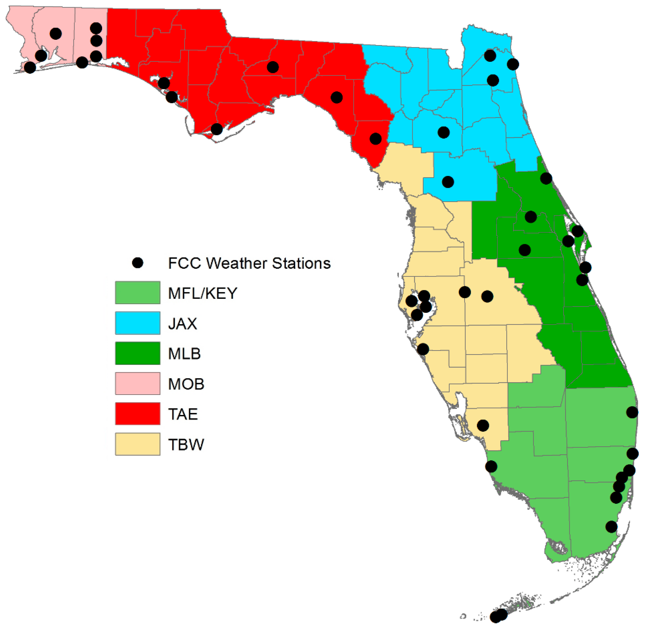
9]. These heat waves were defined using Florida’s National Weather Service (NWS) regions (
Figure 1), combining the small Keys region (KEY) and the Miami region (MFL) to avoid estimation issues due to small counts.
In public health extreme heat morbidity research, two methods are typically used to define a case, or adverse health event. The first method uses all-cause morbidities and includes inpatient hospitalizations and emergency department visits. These studies generally exclude cases described as having external causes of injury [
10], i.e., car accident; however, associations may be difficult to interpret. Other studies use specific groupings of International Classification of Disease (ICD) codes or specific symptoms to focus their studies on illnesses of interest such as exertional heat-related illness, diabetes, cardiovascular diseases, pulmonary diseases, kidney illnesses, and preterm delivery [
1,
2,
3,
5,
6,
11]. These more focused studies typically have motivating biological mechanisms or processes to inform interpretations.
Regardless of how morbidity is defined, most heat wave morbidity research utilizes case-crossover or time-series analysis methods, with no consideration or comparison on which may better reflect the data. Fletcher et al. [
3] performed a time-stratified case-crossover analysis to determine an association between temperatures in July and August, during 1991–2004, with hospital admissions for renal diseases in New York State. Basu et al. [
2] also used a time-stratified case-crossover model to determine associations between high ambient temperature and preterm births in May to September from 1999–2006, in 16 counties in California. Similarly, Tong et al. [
10] used a time-stratified case-crossover analysis to compare the effect of different heat wave definitions on the associations between heat and emergency departments visits. In a later paper, Tong et al. [
12], conducted both time-series and case-crossover analyses to assess short-term association between heat waves and both morbidity and mortality. To estimate the risk of hospitalization for respiratory diseases associated with outdoor heat, Anderson et al. [
1] used a time-series model with the county-level daily hospitalization rate during May to September, from 1999–2008. Modeling the daily number of heat-related emergency department visits during 2007 and 2008, by age group, county and day, a time-series model was also used to estimate the association between average daily mean temperature and heat-related emergency department visits in Lippman et al. [
4].
Leary et al. [
9] were the first to consider and compare multiple methods of imputing missing exposure data for heat waves and was only the second to consider any missing data for heat wave research [
9,
13]. They [
9] showed that the identification of heat waves changed, when considering different imputation methods for missing heat index values. Here, we explore the subsequent changes in inference on heat-related morbidity.
Specifically, we will investigate the effects of missing data and method of analysis on inferences regarding the association between extreme apparent temperature, as measured using heat index, and heat-related morbidity. A strict definition of heat-related morbidity (i.e., inpatient hospitalizations and emergency department visits for heat-related illness) is considered to conservatively assess these associations in Florida from 2005–2012.
2. Experiments
2.1. Exposure Data with Missingness
The Florida Climate Center (FCC) receives weather data from the National Climatic Data Center weather monitors and runs multiple data quality checks while computing additional indicators, such as heat index. Heat index is a measure of how heat is felt by a person, in contrast to measured temperature. Weather data collected from 1973–2012 for 43 weather monitors across the state of Florida were obtained from the FCC. Heat index (°F) was calculated using the standard Rothfusz equation and adjustments, which combine temperature and humidity into a single index [
14]. This study uses the warm season definition created by the FCC, which is from April through September of each year [
15]. The percent missing weather monitor data ranged from 0% to 92% during June through August and from 9% to 96% during April, May, and September.
Assuming the data were missing at random (MAR), the missing data were either (1) ignored or imputed using one of three approaches; (2) a temporal model; (3) a spatial model; and (4) a spatio-temporal model [
8,
9]. Using the distribution of warm season maximum daily heat index for each of the four missing data approaches, 80th percentiles of maximum daily heat indexes during Florida’s warm season were estimated using the observed and imputed data. Using these estimates, heat waves were then defined as a period of consecutive days in which each weather monitor in a region, or the regional average when ignoring missing data, must (a) have the maximum daily heat index above the 80th warm season percentile of heat index; and (b) have at least three days, which need not be consecutive, in the period above a regional upper threshold [
9] (
Table 1). Note that the period of the heat wave differs with imputation method.
2.2. Health Data
In-patient hospitalization and emergency department billing data from 2005 to 2012 were obtained from all Florida hospitals and emergency departments, except state-operated, Federal, or Shriner’s hospitals. These health data were accessed through partnership with the Florida Department of Health; Institutional Review Board approvals and protocols were followed for the Florida Department of Health, the University of Florida, and the University of Missouri.
This study follows the Centers for Disease Control and Prevention (CDC 2013) guidelines for heat-related illness, such that a strict definition using only heat-related ICD-9 codes is used (
Table 2). Patients presenting to a Florida hospital or emergency department from 2005 through 2012 and who have a heat-related ICD-9 code are considered in this study. An indicator variable was created for each imputation approach indicating whether or not the patient was admitted during a heatwave. All non-Florida residents were excluded and the county in Florida associated with the medical record billing address was taken as the patient’s county of residence and used in the analysis. To protect patient confidentiality, county is the geographical area considered for these analyses. External cause of injury code E900.1 is defined as accident due to excessive heat man-made, which could be a burn from a house fire; any billing record with this code was removed. Consequently, 27,934 cases of heat-related morbidity from 2005–2012 were analyzed in this study.
2.3. Linking Health and Exposure Data
Morbidity data are available at the county level, and heat exposure data are reported by individual weather monitors. To link maximum daily heat index to heat-related morbidity at the county level for analysis, block kriging was used to predict the county-level maximum daily heat index based on observed and imputed data from the 43 FCC weather monitors. Block-kriged predictions spatially average the point level estimates from the individual weather monitors and avoid the bias that arises when using the alternative method of aggregation based on county centroids [
16,
17]. However, block kriging requires at least two observations for maximum daily heat index. When less than two observations of maximum daily heat index were recorded for a day, a monitor’s monthly average maximum daily heat index, across years, was taken as that day’s predicted value. This scenario occurred for less than 4% of the data (
n = 43) and never during June, July, or August, typically the warmest months of the defined warm season.
2.4. Case-Crossover Model
The time-stratified case-crossover design is used when a short exposure period causes a change in risk of acute-onset events [
18] and is much like a self-matched case-control design in which every case serves as its own control. The case-crossover design documents exposures immediately prior to the event of interest (called the hazard period) and compares them to exposures from a period during which the event of interest did not occur (called the referent periods). The case-crossover design has previously been applied in studies investigating the association between morbidity and temperature [
3,
10,
12]. Because each case acts as its own control, individual characteristics, such as sex, age, and race, are exactly matched; therefore, the time-stratified case-crossover design inherently controls for confounding effects.
Adapting the notation and likelihood derivation directly from Lu and Zeger [
19], let
be the exposure for person
in county
,
, in interval
, indexed by
i and
c. Using the score function, the estimating equation is the sum, over counties, of the difference between each subject’s exposure at the index time
and a weighted average of all exposures, indexed by
m, at all times in the referent period
; that is,
A time-stratified case-crossover analysis was performed for each region and each method of accounting for missing data. The hazard period and referent periods were linked with the block kriged county maximum daily heat index based on the county of the patients’ billing address and the date of medical service. Referent periods were chosen to be the same day of the week as the hazard period, during the same month [
3,
12]. This controls for day of week effects and results in a maximum of four referent periods for each case period. The Breslow method [
20] was used to minimize any potential exposure bias due to ties [
21] and cubic B-splines, with 3 equally spaced knots, for fixed effects of time are considered. Because of published reports of a lag effect of temperature [
1,
3,
5,
12], lagged-day heat index exposures for block-kriged county daily heat index of same day (no lag), 1-day lag, 2-day lag, and 3-day lag are considered in the analyses.
2.5. Time-Series Model
Time-series analyses are also used to investigate associations between morbidity and periods of extreme heat [
1,
12]. Further, in Lu and Zeger [
19], they demonstrate that when the exposure is common to the cohort at the time (as it is here), that case-crossover approach is equivalent to a log-linear time series analysis. Although the case-crossover analysis controls for confounding by design (through the choice of the referent periods), the time-series approach controls bias through the model itself, i.e., the function of time. This means that the choice of referent intervals in the case-crossover design is equivalent to the choice of estimator for the function of time in a time-series analysis. Let
denote the number of heat-related morbidities on day
t in county
c and let
be the exposures within county
c,
, on day
.
is a nuisance function that is the log of the total population baseline risk for county
c on day
t, which represents factors that affect the population as a whole (improved public health awareness or improved medical services) as well as integrating across the population individual baseline risks, such as demographic factors or smoking habits [
19]. The number of heat-related morbidities for each day
t in each county
c is modeled using log-linear regression techniques, assuming the counts, conditional on the covariates, follow a Poisson distribution. Using these values, the estimating equation to jointly estimate
, the coefficient to determine an association with the exposures, and
is
In addition to the case-crossover analyses, time-series analyses were performed for each region and each method of handling missing data. Numbers of daily heat-related morbidities in a region, were modeled as a function of the block-kriged county maximum daily heat index, based on the county of residence and date, and with indicator variables for the day of the week in each calendar month and year. Similar to the case-crossover analyses, lagged-day heat index exposures for block-kriged county daily heat index of same day (no lag), 1-day lag, 2-day lag, and 3-day lag were considered. Cubic B-splines of time were included as fixed effects in the final time-series models. As is typical for this type of analysis, an overdispersion parameter is added to relax the strong Poisson assumption of equality of mean and variance.
2.6. Zero-Inflated Models
The zero-inflated Poisson model is a mixture model composed of both binary and Poisson processes. One process produces Poisson counts, some of which may be zero, and the other produces zeroes based on a binary process, which may or may not be defined using parameters from the Poisson distribution [
22,
23]. Let
denote the number of heat-related morbidities on day
t in county
c and let
be the exposures within county
c,
, on day
. The Poisson process is assumed to have mean and variance
, where β is the coefficient to determine an association with the exposures and
is a smooth function that represents population baseline risk for county
c on day
t, factors affecting the population as a whole [
19]. The number of heat-related morbidities for each day
t in each county
c is modeled using mixture-model techniques for the zero-inflated Poisson model and its log-likelihood is:
2.7. Truncated Models
The negative binomial model can be written as a Gamma-Poisson mixture distribution and then divided by
to derive the truncated negative binomial model [
24]. Let
denote the number of heat-related morbidities on day
t in county
c,
denote the number of those with no heat-related morbidities on day
t in county
c and let
be the exposures within county
c,
, on day
. The negative binomial process is assumed to have mean and variance
, where β is the coefficient to determine an association with the exposures. The number of heat-related morbidities for each day
t in each county
c is modeled using mixture-model techniques for the truncated negative binomial model and its log-likelihood is:
After comparison between the time-series analysis method and case-crossover method, zero-inflated and truncated model analyses were also performed as a final analysis method for each region using the spatio-temporal method for imputation. For regional analysis, numbers of heat-related morbidities in a region, for each day, were modeled as a function of the block-kriged county maximum daily heat index, based on the county of residence and date, and with indicator variables for the day of the week in each calendar month and year. For statewide analyses, a region variable was added to the model. Similar to all other analyses, lagged-day heat index exposures for block-kriged county daily heat index of same day (no lag), 1-day lag, 2-day lag, and 3-day lag were considered.
3. Results
Case-crossover, time-series, zero-inflated, and truncated models were built for each combination of region and missing data approach. Results for the Jacksonville (JAX) and Melbourne (MLB) NWS regions illustrate the range of inference observed from the NWS regions and are presented to focus the reporting and interpretation of these results to the main recommendations and findings. The JAX region contains five FCC weather monitors within 15 counties and is located in the Northeastern part of Florida. The MLB region contains seven FCC weather monitors within 10 counties and is located in east-central Florida (
Figure 1). For each of the four missing data approaches, regional heat waves and thresholds are provided for the JAX and MLB regions (
Table 1). Heat-related morbidity counts for each NWS region are provided in
Table 3. When multiple heat waves were observed within a region, as in the MLB region, the indicator variable identified whether or not the case was associated with a heat wave and did not differentiate among heat waves.
For these data, inference depended both upon the missing data approach and upon the method of analysis (
Table 4 and
Table 5). Based on the case-crossover analysis, the effect of a heat wave was significant for all methods of considering missing data for both the JAX and MLB regions. However, for the time-series analysis, the main effect of heat wave was not significant with one exception. When the temporal imputation method and time-series model were used for imputation and analysis, respectively, the effect of heat wave was significant for the MLB region, but not for the JAX region. The significances of the effect of the same day, 1-day, 2-day, and 3-day lagged maximum daily heat index, as well as the interactions between heat wave and the same day and lagged heat index, depended upon the method used to handle missing data and on the method of analysis. Significant overdispersion was observed for all time-series analyses, an indication that the case-crossover assumption of a stable exposure distribution is most likely violated, and not otherwise easily checked. Thus, the over-dispersed Poisson time-series model is recommended over the time-stratified case-crossover model.
However, in the model diagnostic plots of residuals against predicted values for the over-dispersed Poisson time-series model for the NWS region, it was evident that the Poisson assumptions were violated. In particular, the plot showed a clear separation by the number of heat events. Thus, this method is not recommended for these data. After several alternative models were considered, including zero-inflated Poisson (ZIP) and zero-inflated negative binomial models (ZINB), truncated Poisson and truncated negative binomial models were used to fit the regional data (
Table 6). Although not recommended as a predictive model, the model diagnostics indicated a much better fit to the heat-related morbidity data, compared to the overdispersed Poisson model (
Table 7). Consequently, the recommended model to assess the association between heat-related morbidity and heat waves across Florida are the truncated models.
A state-wide analysis was also conducted. Leary et al. [
9] recommended that a spatio-temporal model be used to impute missing heat exposure data. Regional analyses indicated that the truncated negative binomial (MLB) or truncated Poisson model (JAX) provides the best fit to heat-related morbidity. In addition, zero-inflated Poisson and zero-inflated negative binomial models were alternatively considered (
Table 8). Similar to the regional analyses, the truncated negative binomial model was determined to provide the best fit to the data.
All models with and without fixed time factors and including indicator variables for day of week, within month and year, were compared using the Akaike Information Criterion (AIC) and Bayesian Information Criterion (BIC), which is appropriate for non-nested model selection [
25]. The AIC and BIC values were similar for the models with indicator variables, both with and without fixed time factors. However, including these estimators for time is necessary because of the potential confounding of the heat index exposure over time and to control for confounding by other, time-varying factors.
Within the statewide truncated negative binomial model, the association between heat-related morbidity and same-day exposure was significant (p ≤ 0.05), indicating that the heat index is associated with morbidity on that day. The statistically significant interactions between same-day exposures and region and between region and heat wave suggest that the effect of heat exposure on the day of morbidity initialization varies with region in the state and that the effect of heat wave on morbidity depends on the region. The presence of the statistically significant interactions between 3-day lagged exposure, region, and heatwave further suggests that the effect of a 3-day lagged heat exposure on morbidity varies with both region and heatwave. Nearly statistically significant interactions were observed between 2-day lagged exposure and region and the 3-way interaction between region, heat wave, and 2-day lagged exposure, indicating that further study is need to fully understand the relationship of sustained heat exposure across region and heat wave.
4. Discussion
Similar to past research, this regional analyses indicated no association between heat wave and heat-related morbidity. However, statewide analyses indicated a regional effect on the association between heat-related morbidity and heat waves. Regional and statewide results from this study indicate differences in public health conclusions when different approaches for missing exposure data and model choice are compared. Recommendations based on these results are to use spatio-temporal methods to impute missing exposure data and to model these data using truncated models to investigate 2005–2012 heat-related morbidity across Florida.
In this study, exposures to heat are defined as county-level maximum daily heat index and are linked to each resident within a county. However, this measure of heat index may not reflect true exposure because residents may spend time indoors during the hottest portion of a day or may travel between counties, a limitation of this study. Although the focus here is the association between an individual’s exposure to extreme heat and heat-related morbidity, the analyses are based on the average county-level exposure and the number of heat-related morbidity cases in a county. Accordingly, drawing inference about individuals using these types of aggregated data can lead to ecological bias [
26].
Heat-related morbidity, using the CDC definition, was considered in this study to identify those health events which are directly related to extreme heat; this health outcome is specific and chosen to focus on health effects with clear causation and for comparison with other heat-related morbidity studies. With respect to estimation and modeling, the daily frequency of heat-related morbidity could affect overdispersion in the models, although a more general health outcome may have a smaller effect, this may not uniformly be the case. For these reasons, overdisperion must be considered in analyses for health outcomes.
Each missing heat index value was imputed once. Because the imputed value was then treated as if it were observed, the standard errors are biased downward, and the p-values associated with the tests of effects in the models are also biased downward. This is a limitation of this study.
In addition, use of air-conditioning (AC) is a mitigating factor for heat-related illness, and AC use is abundant throughout Florida. However, state-wide data that would allow the frequency and level of air-conditioning utilization/usage to be determined are not available so cannot be included in these analyses. Warm and humid weather is not uncommon in Florida, and it is possible that residents may have adapted to such extreme conditions, using additional methods beyond AC use.
Although other factors are important in case-crossover analyses, bias has been shown to be more of a factor for proper estimation, compared to statistical precision [
27]. To mitigate bias, the case-crossover model must appropriately account for the changes in time that confound exposures [
28]. The overdispersion observed for all time-series analyses conducted indicates that, among other issues, the influence of unmeasured time-varying factors is not accounted for by the assumed case-crossover model [
28]. Failing to account for this overdispersion tends to result in standard errors that are biased downwards and, consequently, inflated test statistics. This may be part of the reason that more significant results were obtained for the case-crossover analysis compared to the time-series analysis. As these models are mathematically equivalent, violations in model assumptions is the most likely contributor to differences in results, particularly for the case-crossover method as the assumptions are difficult to assess. Previous studies specific to Florida have concluded that there is no statistically significant increase in mortality during periods of high summertime temperatures [
29]. However, no other study has investigated the effects of heat on heat-specific morbidity for Florida. Statewide truncated negative binomial model results indicated statistically significant associations between heat-related morbidity and regional effects of heat index.
5. Conclusions
This study clearly demonstrates that conclusions about the relationship between public health and environmental factors (here heat effects) can depend on how missing data are accounted for and the choice of model used for analysis. Accounting for both spatial and temporal effects when imputing missing exposure data allowed heat waves to be more accurately determined; ignoring missing data and considering only spatial effects were not acceptable approaches. Here the truncated Poisson and truncated negative binomial models were the only ones that provided an adequate fit of heat-related morbidity to the exposure data. Therefore, to ensure that public health practice is properly informed, the method of imputation and the choice of model should be carefully determined. If valid inference is to be drawn, the fit of the selected model should be carefully evaluated to ensure that it is adequate.
Heat illness is an important public health consideration, especially in Florida, as almost 37% of the total population in Florida is 50 years of age or older. Currently, people 50 and older constitute the largest population demographic [
30] and the biggest economic base in the state [
31]. Adaptation to changing climate—such as increased use of air-conditioning or change in behaviors and the effects of heat on this large, heat-vulnerable population—may not only have important public health implications but also important economic implications for Florida.
Acknowledgments
The authors would like to thank the Florida Department of Health, the University of Florida, and the University of Missouri for their continued support. In addition, the authors would like to thank Babette Brumback, Wendell P. Cropper, Jr., and Xiaohui Xu for critical review of earlier drafts of this work.
Author Contributions
All authors conceived and designed the experiments; E.L. performed the methodology; E.L. and L.J.Y. analyzed the data; M.M.J. and C.D. contributed reagents/materials/analysis tools; E.L. wrote the paper. Authorship must be limited to those who have contributed substantially to the work reported.
Conflicts of Interest
The authors declare no conflict of interest. This project was supported by an award from the Centers for Disease Control and Prevention (grant number U38-EH000941, Florida Environmental Public Health Tracking Network Implementation). The founding sponsors had no role in the design of the study; in the collection, analyses, or interpretation of data; in the writing of the manuscript, and in the decision to publish the results. Its contents are solely the responsibility of the authors and do not necessarily represent the official views of the Centers for Disease Control and Prevention.
References
- Anderson, G.B.; Dominici, F.; Wang, Y.; McCormack, M.C.; Bell, M.L.; Peng, R.D. Heat-related Emergency Hospitalizations for Respiratory Diseases in the Medicare Population. Am. J. Respir. Crit. Care Med. 2013, 187, 1098–1103. [Google Scholar] [CrossRef] [PubMed]
- Basu, R.; Malig, B.; Ostro, B. High Ambient Temperature and the Risk of Preterm Delivery. Am. J. Epidemiol. 2010, 172, 1108–1117. [Google Scholar] [CrossRef] [PubMed]
- Fletcher, B.A.; Lin, S.; Fitzgerald, E.F.; Hwang, S. Association of Summer Temperatures with Hospital Admissions for Renal Diseases in New York State: A Case-crossover Study. Am. J. Epidemiol. 2012, 175, 907–916. [Google Scholar] [CrossRef] [PubMed]
- Lippman, S.; Fuhrmann, C.; Waller, A.; Richardson, D. Ambient Temperature and Emergency Department Visits for Heat-related Illness in North Carolina, 2007–2008. Environ. Res. 2013, 124, 35–42. [Google Scholar] [CrossRef] [PubMed]
- Nitschke, M.; Tucker, G.R.; Hansen, A.L.; Williams, S.; Zhang, Y.; Bi, P. Impact of two recent extreme heat episodes on morbidity and mortality in Adelaide, South Australia: A case-series analysis. Environ. Health 2011, 10, 42. [Google Scholar] [CrossRef] [PubMed]
- Noe, R.S.; Choudhary, E.; Cheng-Dobson, J.; Wolkin, A.F.; Newman, S.B. Exertional Heat-Related Illnesses at the Grand Canyon National Park, 2004–2009. Wilderness Environ. Med. 2013, 24, 422–428. [Google Scholar] [CrossRef] [PubMed]
- NOAA (National Oceanic and Atmospheric Administration). Climate Normals. 2010. Available online: https://www.ncdc.noaa.gov/data-access/land-based-station-data/land-based-datasets/climate-normals (accessed on 15 January 2016).
- Leary, E. Climate Change and Heat Impacts on Health for Florida: A New Methodology and Analysis. Ph.D. Dissertation, University of Florida, Gainesville, FL, USA, August 2014. [Google Scholar]
- Leary, E.; Young, L.J.; DuClos, C.; Jordan, M.M. Identifying Heat Waves in Florida: Considerations of Missing Weather Data. PLoS ONE 2015, 10, e0143471. [Google Scholar] [CrossRef] [PubMed]
- Tong, S.; Wang, X.Y.; Barnett, A.G. Assessment of Heat-related Health Impacts in Brisbane, Australia: Comparison of Different Heatwave Definitions. PLoS ONE 2010, 5, e12155. [Google Scholar] [CrossRef] [PubMed]
- Pantavou, K.; Theoharatos, A.; Santamouris, M. Evaluating Thermal Comfort Conditions and Health Responses during an Extremely Hot Summer in Athens. Build. Environ. 2011, 46, 339–344. [Google Scholar] [CrossRef]
- Tong, S.; Wang, X.Y.; Guo, Y. Assessing the Short-Term Effects of Heatwaves on Mortality and Morbidity in Brisbane, Australia: A Comparison of Case-crossover and Time Series Analysis. PLoS ONE 2012, 7, e37500. [Google Scholar] [CrossRef] [PubMed]
- Deschênes, O.; Greenstone, M. Climate Change, Mortality, and Adaptation: Evidence from Annual Fluctuations in Weather in the US. Am. Econ. J. Appl. Econ. 2011, 3, 152–185. [Google Scholar] [CrossRef]
- Winsberg, M.D.; Simmons, M. An Analysis of the Beginning, End, Length, and Strength of Florida’s Warm Season. Florida Climate Center, 2007. Available online: http://climatecenter.fsu.edu/topics/specials/floridas-hot-season (accessed on 6 April 2014).
- National Weather Service. The Heat Index Equation. Available online: http://www.wpc.ncep.noaa.gov/html/heatindex_equation.shtml (accessed on 3 June 2015).
- Young, L.J.; Gotway, C.A.; Kearney, G.; DuClos, C. Assessing Uncertainty in Support-adjusted Spatial Misalignment Problems. Commun. Stat. Theory Methods 2009, 38, 3249–3264. [Google Scholar] [CrossRef]
- Young, L.J.; Gotway, C.A.; Yang, J.; Kearney, G.; DuClos, C. Linking Health and Environmental Data in Geographical Analysis: It’s So Much More than Centroids. Spat. Spatiotemporal. Epidemiol. 2009, 1, 73–84. [Google Scholar] [CrossRef] [PubMed]
- Maclure, M. The Case-Crossover Design: A Method for Studying Transient Effects on the Risk of Acute Events. Am. J. Epidemiol. 1991, 133, 144–153. [Google Scholar] [CrossRef] [PubMed]
- Lu, Y.; Zeger, S.L. On the equivalence of case-crossover and time series methods in environmental epidemiology. Biostatistics 2007, 8, 337–344. [Google Scholar] [CrossRef] [PubMed]
- Breslow, N.E. Covariance analysis of censored survival data. Biometrics 1974, 30, 89–99. [Google Scholar] [CrossRef] [PubMed]
- Wang, S.V.; Coull, B.A.; Schwartz, J.; Mittleman, M.A.; Wellenis, G.A. Potential for Bias in Case-crossover Studies with Shared Exposures Analyzed Using SAS. Am. J. Epidemiol. 2011, 174, 118–124. [Google Scholar] [CrossRef] [PubMed]
- Lambert, D. Zero-inflated Poisson regression, with an application to defects in manufacturing. Technometrics 1992, 34, 1–14. [Google Scholar] [CrossRef]
- Li, C. Score tests for semiparametric zero-inflated Poisson models. Int. J. Stat. Probab. 2012, 1, 1–7. [Google Scholar] [CrossRef]
- Sampford, M.R. The Truncated Negative Binomial Distribution. Biometrika 1955, 42, 58–69. [Google Scholar] [CrossRef]
- Burnham, K.P.; Anderson, D.R. Model Selection and Multimodel Inference, 2nd ed.; Spring: New York, NY, USA, 2002. [Google Scholar]
- Gotway, C.A.; Young, L.J. Combining incompatible spatial data. J. Am. Stat. Assoc. 2002, 97, 632–648. [Google Scholar] [CrossRef]
- Levy, D.; Lumley, T.; Sheppard, L.; Kaufman, J.; Checkoway, H. Referent selection in case-crossover analyses of acute health effects of air pollution. Epidemiology 2001, 12, 186–192. [Google Scholar] [CrossRef] [PubMed]
- Lu, Y.; Symons, J.M.; Geyh, A.S.; Zeger, S.L. An Approach to Checking Case-Crossover Analyses Based on Equivalence with Time-Series Methods. Epidemiology 2008, 19, 169–175. [Google Scholar] [CrossRef] [PubMed]
- The Center for Science and Public Policy (CSPP). Climate Change in Florida: Is There a Human Footprint in Florida’s Climate History? 2007. Available online: http://ff.org/centers/csspp/pdf/20070709_florida.pdf (accessed on 6 April 2014).
- United States Census Bureau (USCB). 2010. Available online: http://www.census.gov/2010census/popmap/ (accessed on 6 April 2014).
- Florida Climate Alliance. Feeling the Heat in Florida: Global Warming on the Local Level. 2001. Available online: http://www.nrdc.org/globalwarming/florida/florida.pdf (accessed on 6 April 2014).
© 2017 by the authors. Licensee MDPI, Basel, Switzerland. This article is an open access article distributed under the terms and conditions of the Creative Commons Attribution (CC BY) license (http://creativecommons.org/licenses/by/4.0/).


