Enhanced MODIS Atmospheric Total Water Vapour Content Trends in Response to Arctic Amplification

 ,
, 
 , ,
, , 
Abstract
1. Introduction
2. Data Set
2.1. MODIS TCWV
2.2. MODIS Snow Cover
2.3. MODIS Vegetation Index
2.4. MODIS Sea Surface Temperature
2.5. NSIDC Sea Ice Extent
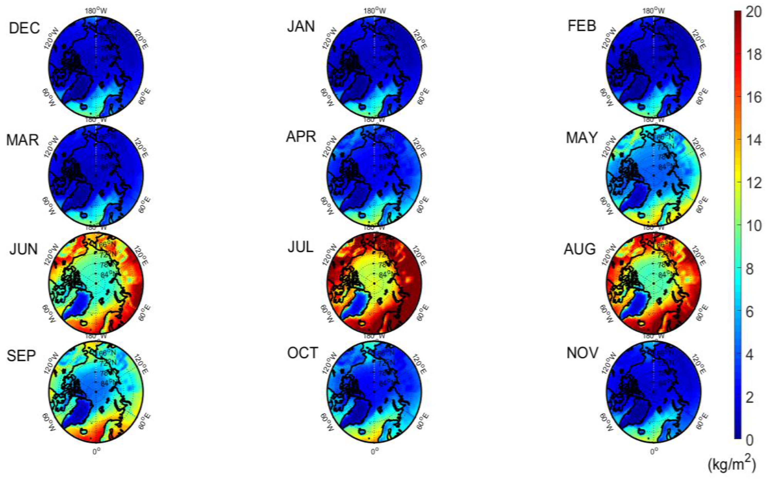
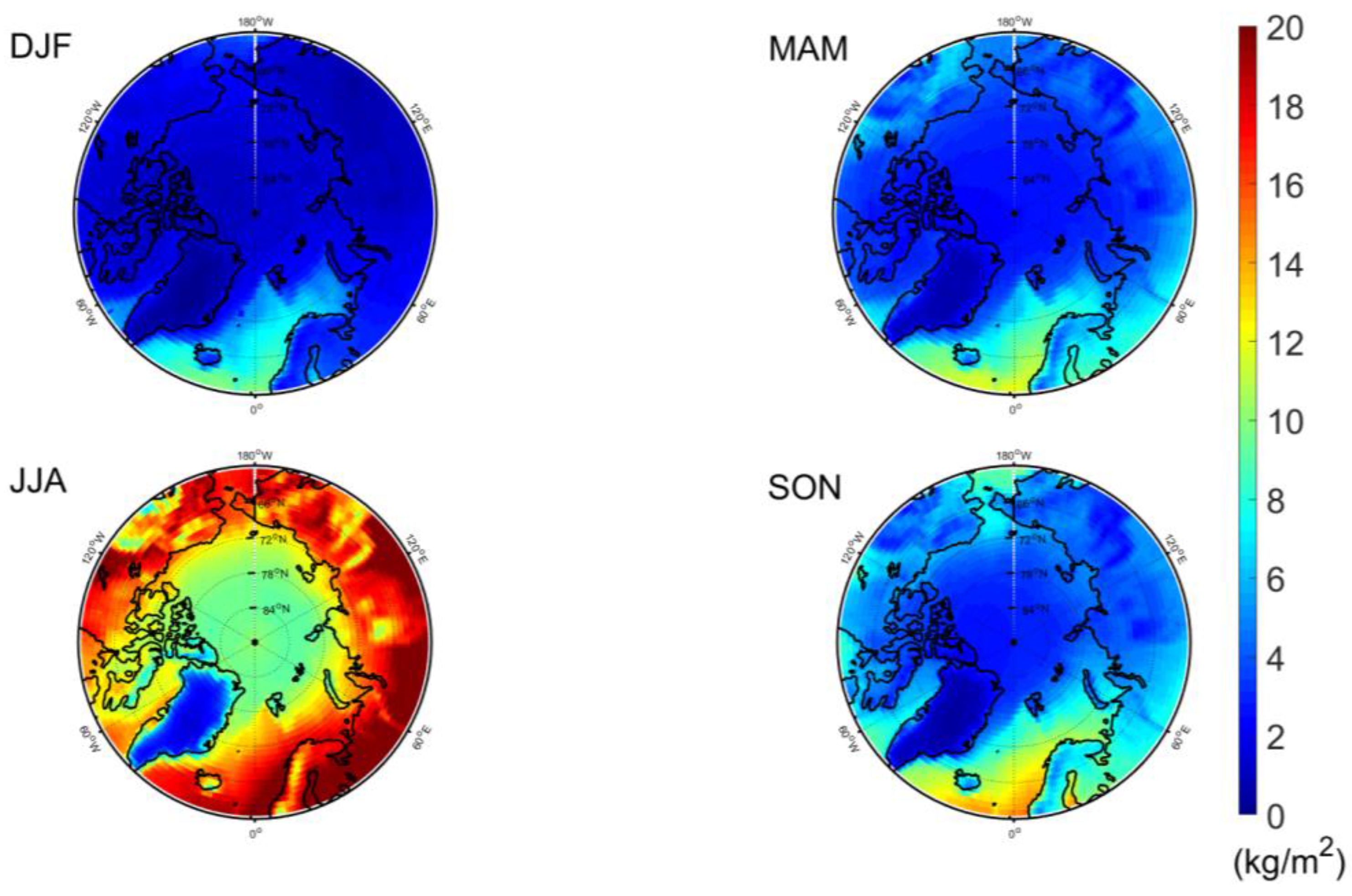
3. TCWV Features
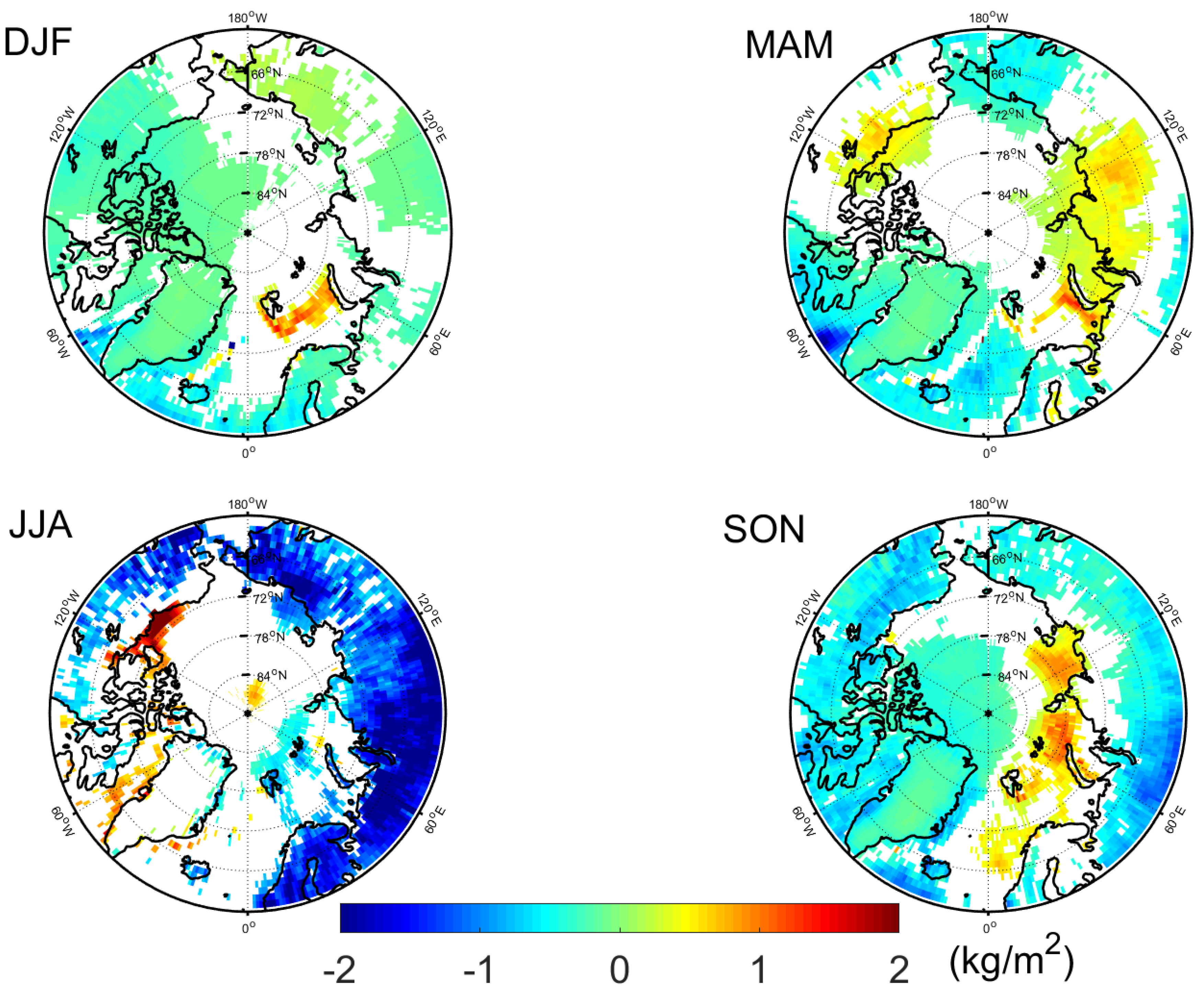
4. TCWV Linear Trends and Discussion
General Discussions
5. TCWV Responses to Arctic Amplification
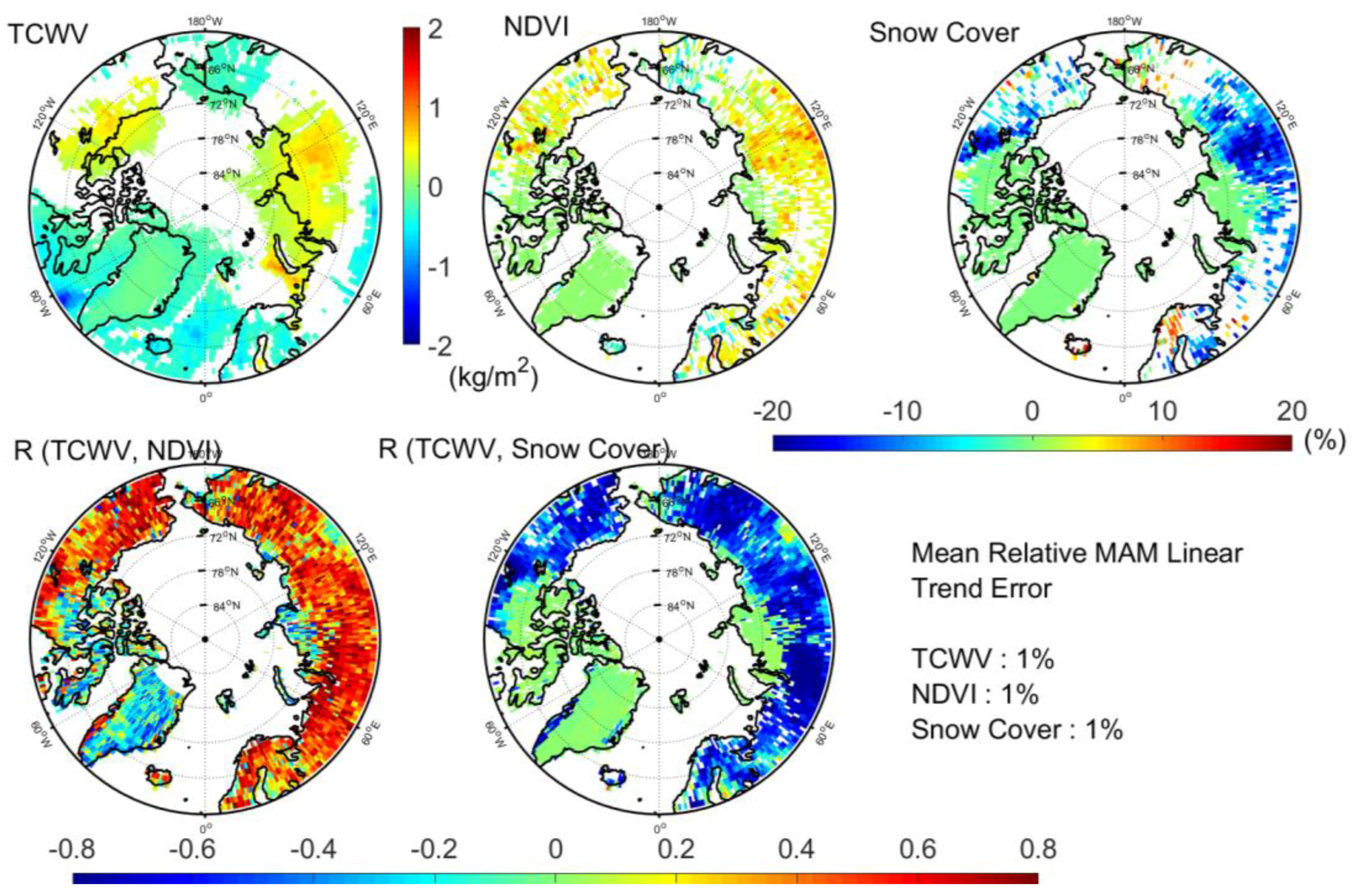
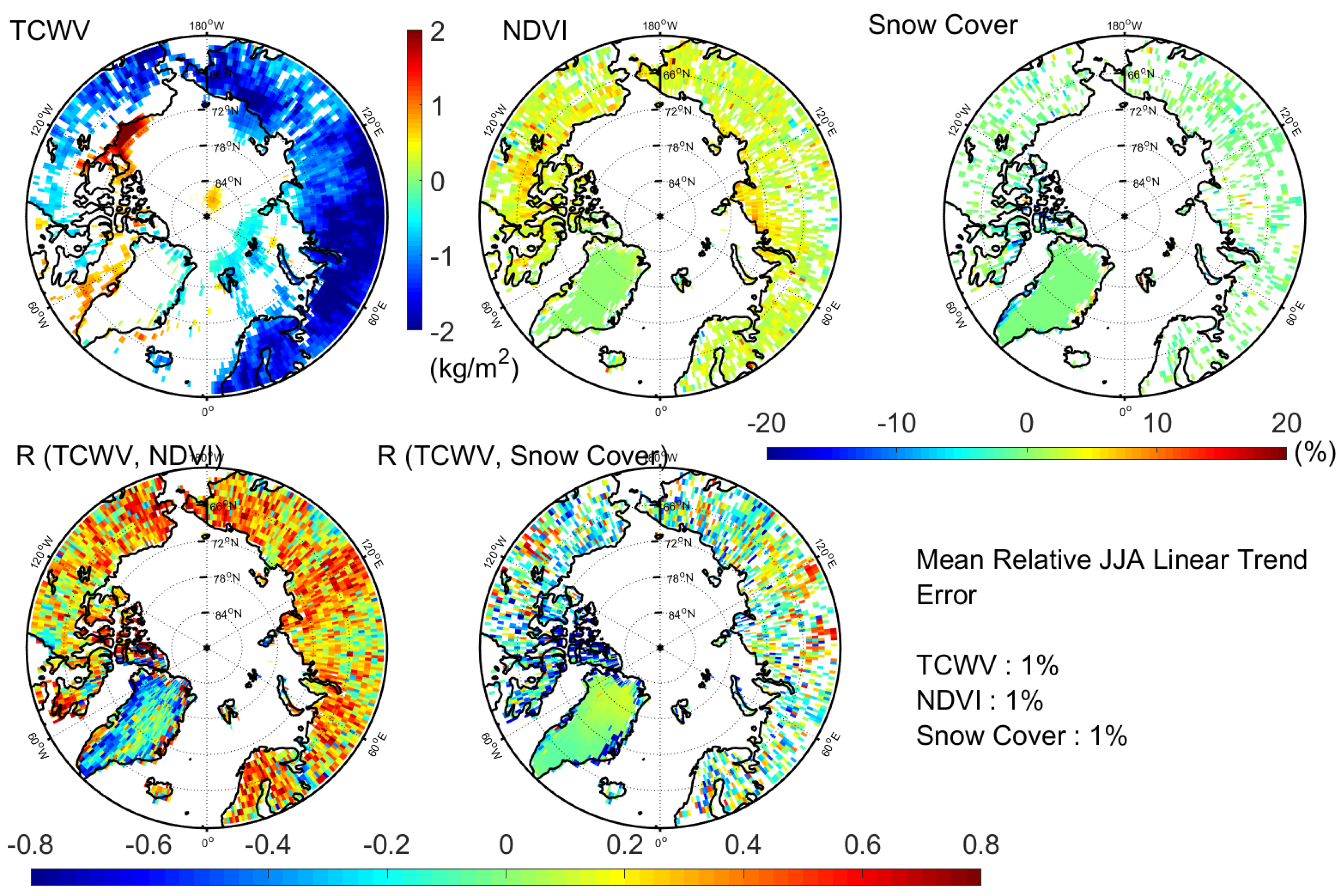
5.1. Spring and Summer TCWV Trends in Response to NDVI and Snow Cover Changes
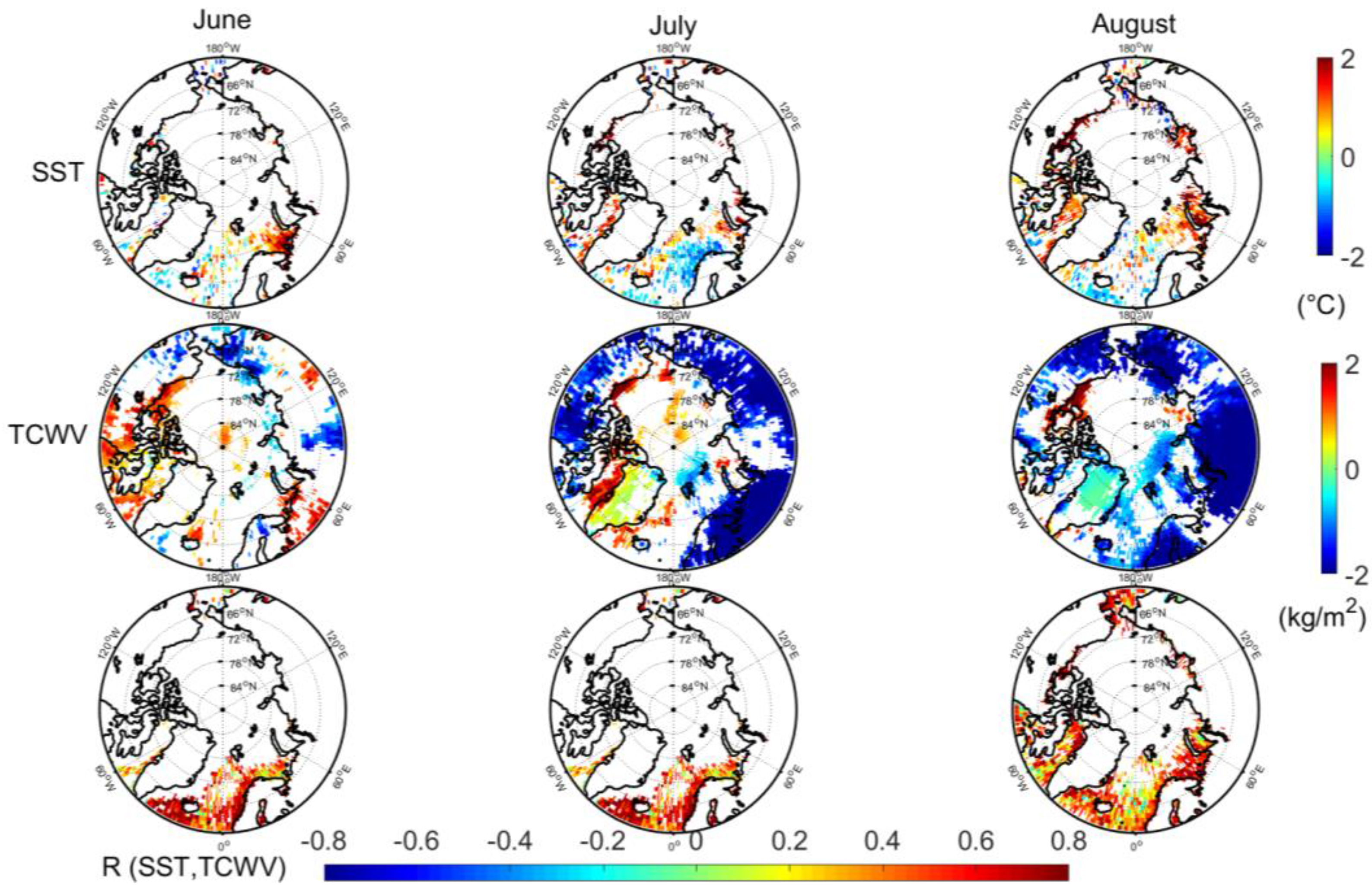
5.2. TCWV Response to Regional Upper Ocean Warming (TCWV Trends in Response to SST Trends)
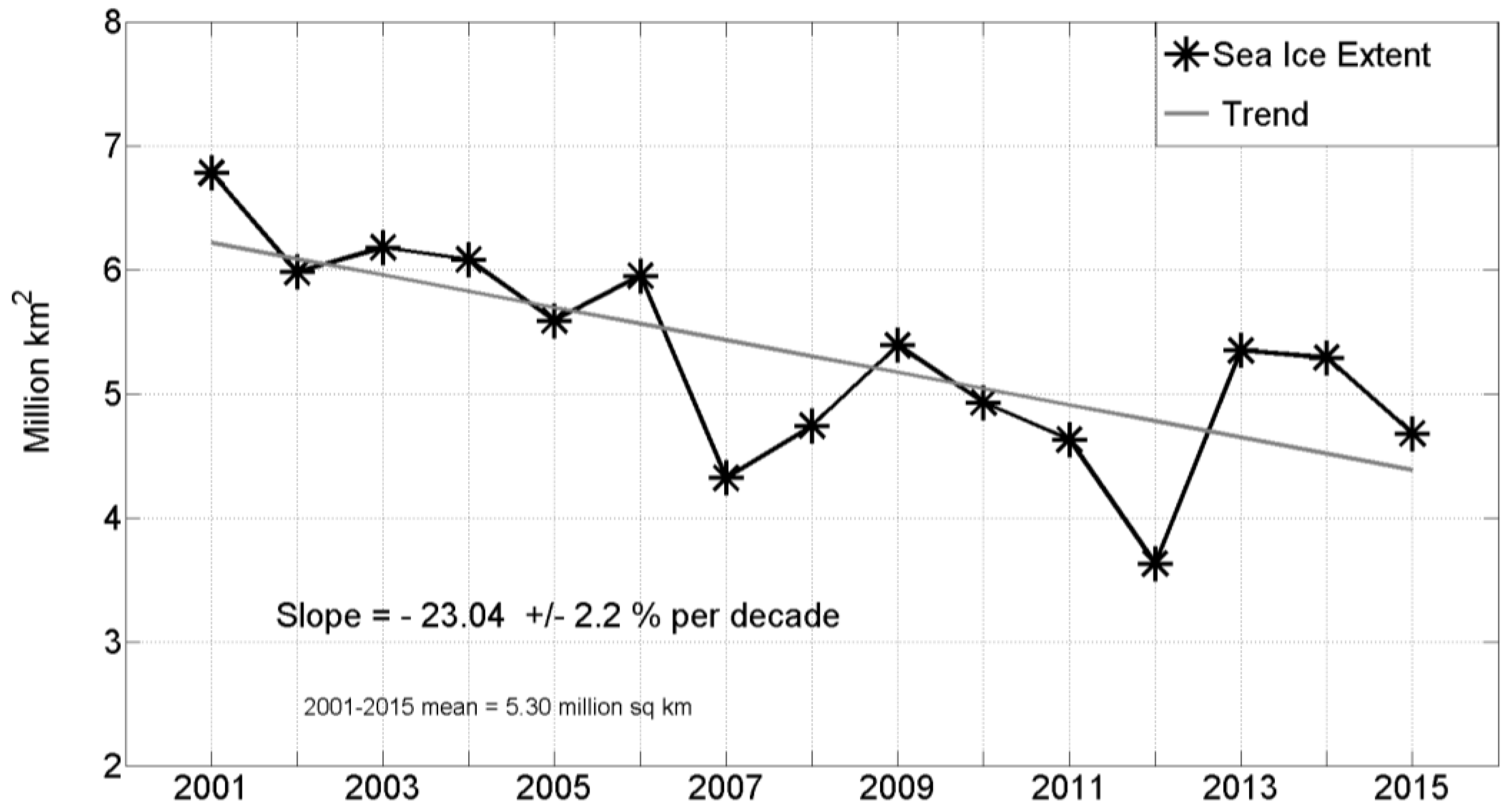
5.3. TCWV Response to Sea Ice Extent Retreat
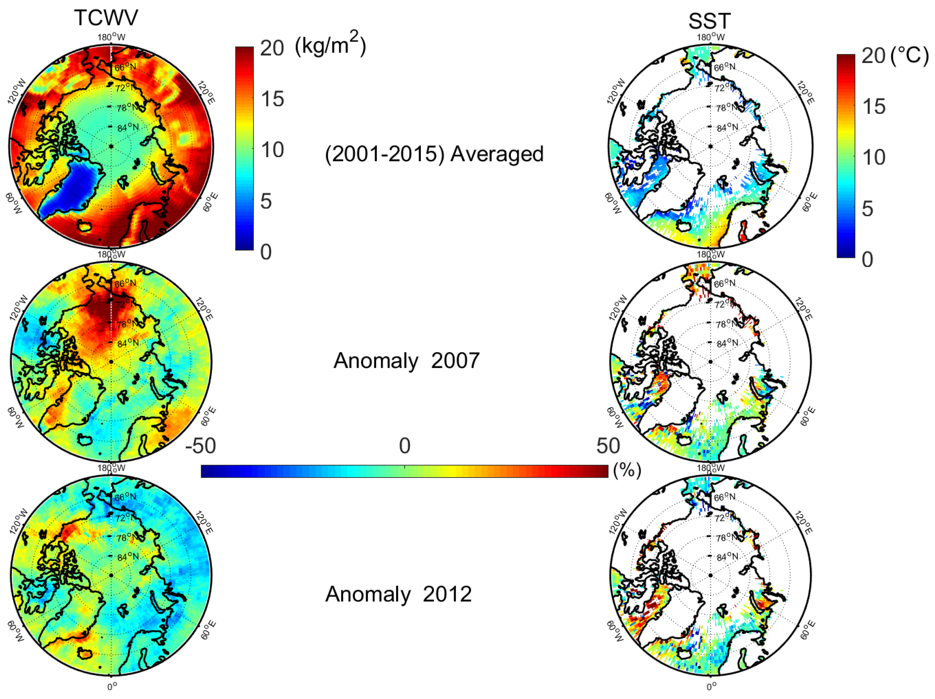
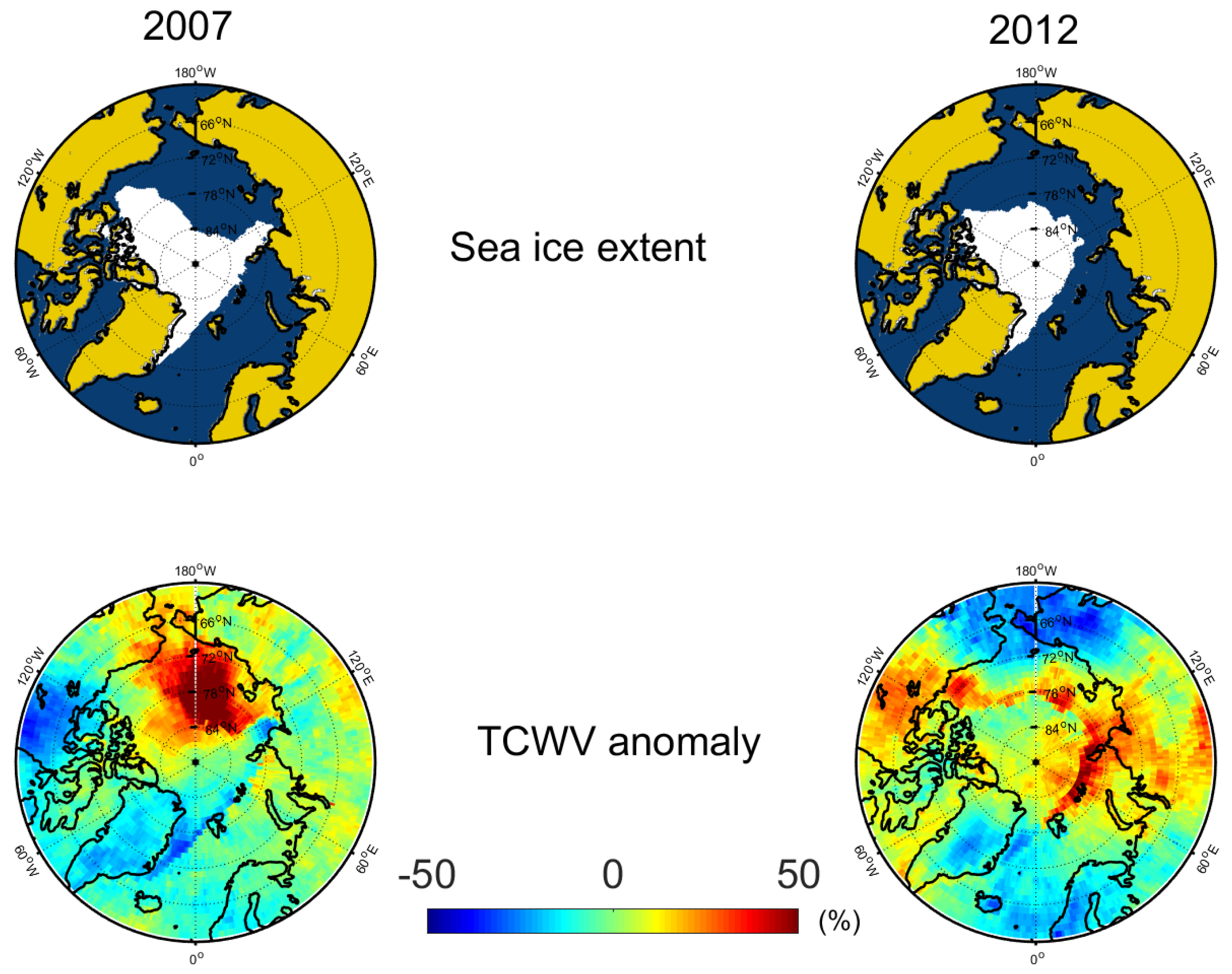
5.3.1. September Sea Ice Extent Decline in 2007 and 2012
5.3.2. Barents and Kara Amplification
6. Conclusions
Acknowledgments
Author Contributions
Conflicts of Interest
References
- Polyakov, I.V.; Alekseev, G.V.; Bekryaev, R.V.; Bhatt, U.; Colony, R.L.; Johnson, M.A.; Karklin, V.P.; Makshtas, A.P.; Walsh, D.; Yulin, A.V. Observationally based assessment of polar amplification of global warming. Geophys. Res. Lett. 2002, 29, 25-1–25-4. [Google Scholar] [CrossRef]
- Serreze, C.M.; Francis, J.A. The Arctic Amplification Debate. Clim. Chang. 2006, 76, 241–264. [Google Scholar] [CrossRef]
- Ghatak, D.; Miller, J. Implications for Arctic amplification of changes in the strength of the water vapor feedback. J. Geophys. Res. Atmos. 2013, 118, 7569–7578. [Google Scholar] [CrossRef]
- Serreze, C.M.; Barrett, A.P.; Stroeve, J.C.; Kindig, D.N.; Holland, M.M. The emergence of surface-based Arctic amplification. Cryosph 2009, 3, 11–19. [Google Scholar] [CrossRef]
- Bekryaev, V.R.; Polyakov, I.V.; Alexeev, V.A. Role of polar amplification in long-term surface air temperature variations and modern arctic warming. J. Clim. 2010, 23, 3888–3906. [Google Scholar] [CrossRef]
- Cohen, J.; Screen, J.A.; Furtado, J.C.; Barlow, M.; Whittleston, D.; Coumou, D.; Francis, J.; Dethloff, K.; Entekhabi, D.; Overland, J.; et al. Recent Arctic amplification and extreme mid-latitude weather. Nat. Geosci. 2014, 7, 627–637. [Google Scholar] [CrossRef]
- Vihma, T. Effects of Arctic Sea Ice Decline on Weather and Climate: A Review. Surv. Geophys. 2014, 35, 1175–1214. [Google Scholar] [CrossRef]
- Screen, A.J.; Simmonds, I. The central role of diminishing sea ice in recent Arctic temperature amplification. Nature 2010, 464, 1334–1337. [Google Scholar] [CrossRef] [PubMed]
- Chen, Y.; Miller, J.R.; Francis, J.A.; Russell, G.L. Projected regime shift in Arctic cloud and water vapor feedbacks. Environ. Res. Lett. 2011, 6, 44007. [Google Scholar] [CrossRef]
- Francis, J.; Hunter, E. Changes in the fabric of the Arctic’s greenhouse blanket. Environ. Res. Lett. 2007, 2, 45011. [Google Scholar] [CrossRef]
- Miller, R.J.; Chen, Y.; Russell, G.L.; Francis, J.A. Future regime shift in feedbacks during Arctic winter. Geophys. Res. Lett. 2007, 34, 7–10. [Google Scholar] [CrossRef]
- Winton, M. Amplified Arctic climate change: What does surface albedo feedback have to do with it. Geophys. Res. Lett. 2006, 33, 1–4. [Google Scholar] [CrossRef]
- Screen, A.J.; Simmonds, I.; Deser, C.; Tomas, R. The atmospheric response to three decades of observed arctic sea ice loss. J. Clim. 2013, 26, 1230–1248. [Google Scholar] [CrossRef]
- Hansen, J.; Sato, M.; Ruedy, R.; Nazarenko, L.; Lacis, A.; Schmidt, G.A.; Russell, G.; Aleinov, L.; Bauer, M.; Bauer, S. Climate and Dynamics-D18104-Efficacy of climate forcings. J. Geophys. Res. D-Atmos. 2005, 110, 18. [Google Scholar] [CrossRef]
- Hansen, J.; Sato, M.; Ruedy, R.; Kharecha, P.; Lacis, A.; Miller, R.; Nazarenko, L.; Lo, K.; Schmidt, G.A.; Russell, G.I.; et al. Dangerous human-made interference with climate: A GISS modelE study. Atmos. Chem. Phys. 2007, 7, 2287–2312. [Google Scholar] [CrossRef]
- Graversen, R.G. Do changes in the midlatitude circulation have any impact on the Arctic surface air temperature trend. J. Clim. 2006, 19, 5422–5438. [Google Scholar] [CrossRef]
- Sherwood, C.S.; Roca, R.; Weckwerth, T.M.; Andronova, N.G. Tropospheric Water Vapor, Convection and Climate. Rev. Geophys. 2010, 48, 1–29. [Google Scholar] [CrossRef]
- Gaffen, J.D.; Robock, A.; Elliott, W.P. Annual cycles of tropospheric water vapor. J. Geophys. Res. 1992, 97, 18185. [Google Scholar] [CrossRef]
- Screen, A.J.; Simmonds, I. Half-century air temperature change above Antarctica: Observed trends and spatial reconstructions. J. Geophys. Res. Atmos. 2012, 117, 16. [Google Scholar] [CrossRef]
- Ross, J.R.; Elliot, W.P. Radiosonde-based Northern Hemisphere tropospheric water vapor trends. J. Clim. 2001, 14, 1602–1612. [Google Scholar] [CrossRef]
- Trenberth, E.K.; Fasullo, J.; Smith, L. Trends and variability in column-integrated atmospheric water vapor. Clim. Dyn. 2005, 24, 741–758. [Google Scholar] [CrossRef]
- Mieruch, S.; Noël, S.; Bovensmann, H.; Burrows, J.P. Analysis of global water vapour trends from satellite measurements in the visible spectral range. Atmos. Chem. Phys. 2008, 8, 491–504. [Google Scholar] [CrossRef]
- Boisvert, N.L.; Stroeve, J.C. The Arctic is becoming warmer and wetter as revealed by the Atmospheric Infrared Sounder. Geophys. Res. Lett. 2015, 42, 4439–4446. [Google Scholar] [CrossRef]
- Boisvert, N.L.; Markus, T.; Vihma, T. Moisture flux changes and trends for the entire Arctic in 2003–2011 derived from EOS Aqua data. J. Geophys. Res. Ocean. 2013, 118, 5829–5843. [Google Scholar] [CrossRef]
- Serreze, C.M.; Barrett, A.P.; Stroeve, J. Recent changes in tropospheric water vapor over the Arctic as assessed from radiosondes and atmospheric reanalyses. J. Geophys. Res. Atmos. 2012, 117, 10. [Google Scholar] [CrossRef]
- Gao, B.C. Water vapor retrievals using Moderate Resolution Imaging Spectroradiometer (MODIS) near-infrared channels. J. Geophys. Res. 2003, 108, 1–10. [Google Scholar] [CrossRef]
- Alraddawi, D.; Sarkissian, A.; Keckhut, P.; Bock, O.; Noël, S.; Bekki, S.; Irbah, A.; Meftah, M.; Claud, C. Comparison of total water vapour content in the Arctic derived from GPS, AIRS, MODIS and SCIAMACHY. Atmos. Meas. Tech. Discuss. 2017, 5194. [Google Scholar] [CrossRef]
- Hall, K.D.; Riggs, G.A. Accuracy assessment of the MODIS snow products. Hydrol. Process. 2007, 21, 1534–1547. [Google Scholar] [CrossRef]
- Platnick, S.; King, M.D.; Ackerman, S.A.; Menzel, W.P.; Baum, B.A.; Riédi, J.C.; Frey, R.A. The MODIS cloud products: Algorithms and examples from terra. IEEE Trans. Geosci. Remote Sens. 2003, 41, 459–472. [Google Scholar] [CrossRef]
- Huete, A.; Justice, C. Modis Vegetation Index Algorithm Theoretical Basis. Environ. Sci. 1999, 13, 129. [Google Scholar] [CrossRef]
- Stow, A.D.; Hope, A.; McGuire, D.; Verbyla, D.; Gamon, J.; Huemmrich, F.; Houston, S.; Racine, C.; Sturm, M.; Tape, K.; et al. Remote sensing of vegetation and land-cover change in Arctic Tundra Ecosystems. Remote Sens. Environ. 2004, 89, 281–308. [Google Scholar] [CrossRef]
- Fetterer, F.; Knowles, K.; Meier, W.; Savoie, M. Sea Ice Index, Version 2; National Snow and Ice Data Center: Boulder, CO, USA, 2016. [Google Scholar] [CrossRef]
- Mortin, J.; Howell, S.E.L.; Wang, L.; Derksen, C.; Svensson, G.; Graversen, R.G.; Schrøder, T.M. Extending the QuikSCAT record of seasonal melt–freeze transitions over Arctic sea ice using ASCAT. Remote Sens. Environ. 2014, 141, 214–230. [Google Scholar] [CrossRef]
- Fichot, G.C.; Kaiser, K.; Hooker, S.B.; Amon, R.M.W.; Babin, M.; Bélanger, S.; Walker, S.A.; Benner, R. Pan-Arctic distributions of continental runoff in the Arctic Ocean. Sci. Rep. 2013, 3, 1053. [Google Scholar] [CrossRef] [PubMed]
- Jakobson, E.; Vihma, T. Atmospheric moisture budget in the Arctic based on the ERA-40 reanalysis. Int. J. Climatol. 2010, 30, 2175–2194. [Google Scholar] [CrossRef]
- Held, M.I.; Soden, B.J. Robust responses of the hydrologic cycle to global warming. J. Clim. 2006, 19, 5686–5699. [Google Scholar] [CrossRef]
- López-Moreno, I.J.; Boike, J.; Sanchez-Lorenzo, A.; Pomeroy, J.W. Impact of climate warming on snow processes in Ny-Ålesund, a polar maritime site at Svalbard. Glob. Planet. Chang. 2016, 146, 10–21. [Google Scholar] [CrossRef]
- Onarheim, H.I.; Smedsrud, L.H.; Ingvaldsen, R.B.; Nilsen, F. Loss of sea ice during winter north of Svalbard. Tellus Ser. A Dyn. Meteorol. Oceanogr. 2014, 66, 23933. [Google Scholar] [CrossRef]
- Stroeve, C.J.; Markus, T.; Boisvert, L.; Miller, J.; Barrett, A. Changes in Arctic melt season and implifications for sea ice loss. Geophys. Res. Lett. 2014, 41, 1216–1225. [Google Scholar] [CrossRef]
- Doxaran, D.; Devred, E.; Babin, M. A 50% increase in the mass of terrestrial particles delivered by the Mackenzie River into the Beaufort Sea (Canadian Arctic Ocean) over the last 10 years. Biogeosciences 2015, 12, 3551–3565. [Google Scholar] [CrossRef]
- Markus, T.; Stroeve, J.C.; Miller, J. Recent changes in Arctic sea ice melt onset, freezeup, and melt season length. J. Geophys. Res. Ocean. 2009, 114, 1–14. [Google Scholar] [CrossRef]
- Maslanik, A.J.; Fowler, C.; Stroeve, J.; Drobot, S.; Zwally, J.; Yi, D.; Emery, W. A younger, thinner Arctic ice cover: Increased potential for rapid, extensive sea-ice loss. Geophys. Res. Lett. 2007, 34, 2004–2008. [Google Scholar] [CrossRef]
- Woodgate, A.R.; Aagaard, K.; Weingartner, T.J. Interannual changes in the Bering Strait fluxes of volume, heat and freshwater between 1991 and 2004. Geophys. Res. Lett. 2006, 33, 2–6. [Google Scholar] [CrossRef]
- Fettweis, X.; Hanna, E.; Lang, C.; Belleflamme, A.; Erpicum, M.; Gallée, H. Brief communication; Important role of the mid-tropospheric atmospheric circulation in the recent surface melt increase over the Greenland ice sheet. Cryosphere 2013, 7, 241–248. [Google Scholar] [CrossRef]
- Bennartz, R.; Shupe, M.D.; Turner, D.D.; Walden, V.P.; Steffen, K.; Cox, C.J.; Kulie, M.S.; Miller, N.B.; Pettersen, C. July 2012 Greenland melt extent enhanced by low-level liquid clouds. Nature 2013, 496, 83–86. [Google Scholar] [CrossRef] [PubMed]
- Hanna, E.; Fettweis, X.; Mernild, S.H.; Cappelen, J.; Ribergaard, M.H.; Shuman, C.A.; Steffen, K.; Wood, L.; Mote, T.L. Atmospheric and oceanic climate forcing of the exceptional Greenland ice sheet surface melt in summer 2012. Int. J. Climatol. 2014, 34, 1022–1037. [Google Scholar] [CrossRef]
- Luo, B.; Luo, D.; Wu, L.; Zhong, L.; Simmonds, I. Atmospheric circulation patterns which promote winter Arctic sea ice decline. Environ. Res. Lett. 2017, 12, 54017. [Google Scholar] [CrossRef]
- Lee, S.; Gong, T.; Feldstein, S.B.; Screen, J.; Simmonds, I. Revisiting the cause of the 1989-2009 Arctic surface warming using the surface energy budget: downward infrared radiation dominates the surface fluxes. Geophys. Res. Lett. 2017, 44, 10654–10661. [Google Scholar] [CrossRef]
- Simmonds, I. Comparing and contrasting the behaviour of Arctic and Antarctic sea ice over the 35 year period 1979-2013. Ann. Glaciol. 2015, 56, 18–28. [Google Scholar] [CrossRef]
- Vihma, T.; Screen, J.; Tjernström, M.; Newton, B.; Zhang, X.; Popova, V.; Deser, C.; Holland, M.; Prowse, T. The atmospheric role in the Arctic water cycle: A review on processes, past and future changes, and their impacts. J. Geophys. Res. G Biogeosci. 2016, 121, 586–620. [Google Scholar] [CrossRef]
- Blunden, J.; Arndt, D.S.; Blunden, J.; Arndt, D.S. State of the Climate in 2015. Bull. Am. Meteorol. Soc. 2016, 97, Si-S275. [Google Scholar] [CrossRef]
- Webb, E.E.; Schuur, E.A.G.; Natali, S.M.; Oken, K.L.; Bracho, R.; Krapek, J.P.; Risk, D.; Nickerson, N.R. Increased wintertime CO2 loss as a result of sustained tundra warming. J. Geophys. Res. Biogeosci. 2016, 121, 249–265. [Google Scholar] [CrossRef]
- Schaefer, K.; Lantuit, H.; Romanovsky, V.E.; Schuur, E.A.G.; Witt, R. The impact of the permafrost carbon feedback on global climate. Environ. Res. Lett. 2014, 9, 85003. [Google Scholar] [CrossRef]
- Biskaborn, K.B.; Lanckman, J.P.; Lantuit, H.; Elger, K.; Streletskiy, D.A.; Cable, W.L.; Romanovsky, V.E. The new database of the Global Terrestrial Network for Permafrost (GTN-P). Earth Syst. Sci. Data 2015, 7, 745–759. [Google Scholar] [CrossRef]
- Overland, E.J.; Wang, M.; Salo, S. The recent Arctic warm period. Tellus Ser. A Dyn. Meteorol. Oceanogr. 2008, 60, 589–597. [Google Scholar] [CrossRef]
- Perovich, K.D.; Richeter-Menge, J.A.; Jones, K.F.; Light, B. Sunlight, water, and ice: Extreme Arctic sea ice melt during the summer of 2007. Geophys. Res. Lett. 2008, 35, 2–5. [Google Scholar] [CrossRef]
- Bunn, G.A.; Goetz, S.J. Trends in satellite-observed circumpolar photosynthetic activity from 1982 to 2003: The influence of seasonality, cover type, and vegetation density. Earth Interact. 2006, 10, 1–19. [Google Scholar] [CrossRef]
- Beck, A.P.S.; Goetz, S.J. Satellite observations of high northern latitude vegetation productivity changes between 1982 and 2008: Ecological variability and regional differences. Environ. Res. Lett. 2012, 7, 29501. [Google Scholar] [CrossRef]
- Bhatt, S.U.; Walker, D.A.; Raynolds, M.K.; Comiso, J.C.; Epstein, H.E.; Jia, G.; Gens, R.; Pinzon, J.E.; Tucker, C.J.; Tweedie, C.E.; et al. Circumpolar Arctic tundra vegetation change is linked to sea ice decline. Earth Interact. 2010, 14, 1–20. [Google Scholar] [CrossRef]
- Myers-Smith, H.I.; Forbes, B.C.; Wilmking, M.; Hallinger, M.; Lantz, T.; Blok, D.; Tape, K.D.; Macias-Fauria, M.; Sass-Klaassen, U.; Lévesque, E.; et al. Shrub expansion in tundra ecosystems: Dynamics, impacts and research priorities. Environ. Res. Lett. 2011, 6, 45509. [Google Scholar] [CrossRef]
- Tape, D.K.; Gustine, D.D.; Ruess, R.W.; Adams, L.G.; Clark, J.A. Correction: Range expansion of moose in Arctic Alaska linked to warming and increased shrub habitat. PLoS ONE 2016, 11, e0160049. [Google Scholar] [CrossRef] [PubMed]
- Chapin, S.F. Role of Land-Surface Changes in Arctic Summer Warming. Science 2005, 310, 657–660. [Google Scholar] [CrossRef] [PubMed]
- Blok, D.; Heijmans, M.M.P.D.; Schaepman-Strub, G.; Kononov, A.V.; Maximov, T.C.; Berendse, F. Shrub expansion may reduce summer permafrost thaw in Siberian tundra. Glob. Chang. Biol. 2010, 16, 1296–1305. [Google Scholar] [CrossRef]
- Blok, D.; Schaepman-Strub, G.; Bartholomeus, H.; Heijmans, M.M.P.D.; Maximov, T.C.; Berendse, F. The response of Arctic vegetation to the summer climate: Relation between shrub cover, NDVI, surface albedo and temperature. Environ. Res. Lett. 2011, 6, 35502. [Google Scholar] [CrossRef]
- Loranty, M.M.; Goetz, S.J.; Beck, P.S.A. Tundra vegetation effects on pan-Arctic albedo. Environ. Res. Lett. 2011, 6, 29601. [Google Scholar] [CrossRef]
- Myers-Smith, H.I.; Hik, D.S. Shrub canopies influence soil temperatures but not nutrient dynamics: An experimental test of tundra snow-shrub interactions. Ecol. Evol. 2013, 3, 3683–3700. [Google Scholar] [CrossRef] [PubMed]
- Piao, S.; Wang, X.; Ciais, P.; Zhu, B.; Wang, T.; Liu, J. Changes in satellite-derived vegetation growth trend in temperate and boreal Eurasia from 1982 to 2006. Glob. Chang. Biol. 2011, 17, 3228–3239. [Google Scholar] [CrossRef]
- Buermann, W.; Parida, B.; Jung, M.; MacDonald, G.M.; Tucker, C.J.; Reichstein, M. Recent shift in Eurasian boreal forest greening response may be associated with warmer and drier summers. Geophys. Res. Lett. 2014, 41, 1995–2002. [Google Scholar] [CrossRef]
- Kay, E.J.; L’Ecuyer, T.; Gettelman, A.; Stephens, G.; O’Dell, C. The contribution of cloud and radiation anomalies to the 2007 Arctic sea ice extent minimum. Geophys. Res. Lett. 2008, 35, 1–5. [Google Scholar] [CrossRef]
- Parkinson, L.C.; Comiso, J.C. On the 2012 record low Arctic sea ice cover: Combined impact of preconditioning and an August storm. Geophys. Res. Lett. 2013, 40, 1356–1361. [Google Scholar] [CrossRef]
- Dufour, A.; Zolina, O.; Gulev, S.K. Atmospheric moisture transport to the arctic: Assessment of reanalyses and analysis of transport components. J. Clim. 2016, 29, 5061–5081. [Google Scholar] [CrossRef]
- Comiso, C.J. Large decadal decline of the arctic multiyear ice cover. J. Clim. 2012, 25, 1176–1193. [Google Scholar] [CrossRef]
- Maslanik, J.; Stroeve, J.; Fowler, C.; Emery, W. Distribution and trends in Arctic sea ice age through spring 2011. Geophys. Res. Lett. 2011, 38, 2–7. [Google Scholar] [CrossRef]
- Stroeve, J.; Serreze, M.; Drobot, S.; Gearheard, S.; Holland, M.; Masalink, J.; Meier, W.; Scambos, T. Arctic sea ice extent plummets in 2007. Geophys. Res. Lett. 2008, 89, 13–20. [Google Scholar] [CrossRef]
- Comiso, C.J.; Parkinson, C.L.; Gersten, R.; Stock, L. Accelerated decline in the Arctic sea ice cover. Geophys. Res. Lett. 2008, 35, 1. [Google Scholar] [CrossRef]
- Stroeve, C.J.; Kattsov, V.; Barrett, A.; Serreze, M.; Pavlova, T.; Holland, M.; Meier, W.N. Trends in Arctic sea ice extent from CMIP5, CMIP3 and observations. Geophys. Res. Lett. 2012, 39, 1–7. [Google Scholar] [CrossRef]
- Mioche, G.; Jourdan, O.; Ceccaldi, M.; Delano, J. Variability of mixed-phase clouds in the Arctic with a focus on the Svalbard region: A study based on spaceborne active remote sensing. Atmos. Chem. Phys. 2015, 15, 2445–2461. [Google Scholar] [CrossRef]
- Park, R.D.; Lee, S.; Feldstein, S.B. Attribution of the Recent Winter Sea Ice Decline over the Atlantic Sector of the Arctic Ocean. J. Clim. 2015, 28, 4027–4033. [Google Scholar] [CrossRef]
- Maturilli, M.; Herber, A.; König-langlo, G. Surface Radiation Climatology for Ny-Ålesund, Svalbard (78.9° N), Basic Observations for Trend Detection. Theor. Appl. Climatol. 2015, 120, 331–339. [Google Scholar] [CrossRef]


| Region | Latitude Range | Longitude Range |
|---|---|---|
| Barents | 75° N–79° N | 30° E–34° E |
| Kara | 76° N–80° N | 85° E–89° E |
© 2017 by the authors. Licensee MDPI, Basel, Switzerland. This article is an open access article distributed under the terms and conditions of the Creative Commons Attribution (CC BY) license (http://creativecommons.org/licenses/by/4.0/).
Share and Cite
Alraddawi, D.; Keckhut, P.; Sarkissian, A.; Bock, O.; Irbah, A.; Bekki, S.; Claud, C.; Meftah, M. Enhanced MODIS Atmospheric Total Water Vapour Content Trends in Response to Arctic Amplification. Atmosphere 2017, 8, 241. https://doi.org/10.3390/atmos8120241
Alraddawi D, Keckhut P, Sarkissian A, Bock O, Irbah A, Bekki S, Claud C, Meftah M. Enhanced MODIS Atmospheric Total Water Vapour Content Trends in Response to Arctic Amplification. Atmosphere. 2017; 8(12):241. https://doi.org/10.3390/atmos8120241
Chicago/Turabian StyleAlraddawi, Dunya, Philippe Keckhut, Alain Sarkissian, Olivier Bock, Abdanour Irbah, Slimane Bekki, Chantal Claud, and Mustapha Meftah. 2017. "Enhanced MODIS Atmospheric Total Water Vapour Content Trends in Response to Arctic Amplification" Atmosphere 8, no. 12: 241. https://doi.org/10.3390/atmos8120241
APA StyleAlraddawi, D., Keckhut, P., Sarkissian, A., Bock, O., Irbah, A., Bekki, S., Claud, C., & Meftah, M. (2017). Enhanced MODIS Atmospheric Total Water Vapour Content Trends in Response to Arctic Amplification. Atmosphere, 8(12), 241. https://doi.org/10.3390/atmos8120241