Diagnosing Lee Wave Rotor Onset Using a Linear Model Including a Boundary Layer

Abstract

A linear model is used to diagnose the onset of rotors in flow over 2D hills, for atmospheres that are neutrally stratified near the surface and stably stratified aloft, with a sharp temperature inversion in between, where trapped lee waves may propagate. This is achieved by coupling an inviscid two-layer mountain-wave model and a bulk boundary-layer model. The full model shows some ability to diagnose flow stagnation associated with rotors as a function of key input parameters, such as the Froude number and the height of the inversion, in numerical simulations and laboratory experiments carried out by previous authors. While calculations including only the effects of mean flow attenuation and velocity perturbation amplification within the surface layer represent flow stagnation fairly well in the more non-hydrostatic cases, only the full model, taking into account the feedback of the surface layer on the inviscid flow, satisfactorily predicts flow stagnation in the most hydrostatic case, although the corresponding condition is unable to discriminate between rotors and hydraulic jumps. Versions of the model not including this feedback severely underestimate the amplitude of trapped lee waves in that case, where the Fourier transform of the hill has zeros, showing that those waves are not forced directly by the orography.

1. Introduction

Lee wave rotors are elongated vortices formed beneath trapped lee waves generated downstream of quasi-2D mountains, with horizontal axes roughly aligned with the orography [1]. These flow structures, where the flow stagnates and reverses near the surface, are often characterized by flow unsteadiness and turbulence, constituting a serious aviation safety hazard [2,3]. However, they are hard to forecast, because their scale is relatively small (at most, a few km across), and therefore, they are inadequately resolved not only by global, but even by most regional weather prediction models.

The nature of rotors, with flow stagnation and reversal, suggests that they are intrinsically nonlinear phenomena. For this reason and also because the associated turbulence, which affects the large-scale flow, is intrinsically 3D, their detailed forecast is probably only possible using high-resolution numerical simulations, with grid spacings smaller than 1 km and resolving at least part of the turbulence (e.g., Large-Eddy Simulations – LES) [4,5,6].

However, the onset of rotors is ultimately triggered by flow stagnation in quasi-steady flow over quasi-2D orography, a flow configuration that is much simpler than the one arising after the rotors have become turbulent and which may probably be understood using more rudimentary tools. Since carrying out high-resolution numerical simulations is computationally expensive, it would be advantageous if simpler methods could be employed to understand and predict rotor onset.

The fact that the near-surface flow stagnation that is required for rotor onset has been observed and simulated for relatively modest mountain heights (e.g., [7,8]) suggests that the flow may be nearly linear outside the boundary layer in many situations of practical interest and only boundary layer effects induce nonlinearity, with friction facilitating flow stagnation.

It is well-known that the balance of forces within a boundary layer is different from that outside it. In the free atmosphere, the flow is approximately inviscid, satisfying Bernoulli’s equation, i.e., the flow velocity is a minimum where pressure is a maximum. Inside the boundary layer, by contrast, the balance of forces is such that the flow tends to be partially directed towards lower pressures, much as occurs in a more pronounced way in flow inside a vegetation canopy [9]. This has implications for the onset of flow stagnation beneath trapped lee waves, because these waves induce pressure oscillations at the surface, which therefore lead to the possibility of flow stagnation and recirculation.

An alternative way of seeing the problem is by analogy with flow over hills. Flow over a succession of hills is in some sense analogous to flow beneath a trapped lee wave, since both are characterized by an oscillating pressure pattern at the surface, which in the case of hills attains minima over the hill tops. It is known from studies of flow over hills that the existence of a boundary layer has the effect of decelerating the mean incoming flow near the surface while concurrently amplifying the flow perturbation induced by the hill [10]. This is clearly conducive to a higher likeliness of flow stagnation, since stagnation occurs when the velocity perturbation is of equal value and opposite sign to the incoming flow velocity.

It was seen in previous investigations that linear theory can give valuable qualitative indications about the onset of flow stagnation outside the boundary layer [11]. On the other hand, the drag calculations of Teixeira et al. [12] suggested a significant correlation between trapped lee wave drag, calculated using an inviscid model, and the onset of rotors. This is not surprising, since flow stagnation is largely driven by the pressure fluctuations associated with the trapped lee waves, which are also responsible for the drag, as argued above and supported by the results of Vosper et al. [13].

This suggests the approach adopted here, where the inviscid linear model of trapped lee waves over 2D orography developed by Teixeira et al. [12] (hereafter, TAM13) is coupled with a very simple representation of the velocity boundary layer, following Smith et al. [14] (hereafter, SJD06). The idea of coupling an inviscid trapped lee wave model with a boundary layer model for simulating rotors is not wholly new, having been followed by Vosper et al. [13], who adopted the linear boundary layer model of Hunt et al. [15] for that purpose. However, that model is rather complex and turned out to be too cumbersome for a systematic exploration of parameter space.

The aim here is to develop a simpler model that is easy and quick to use for a wide range of input conditions and can provide predictions for the onset of rotors that have qualitative and even some quantitative skill. The main limitation of this model, as formulated here, is that it assumes a specific type of atmospheric profile (nevertheless fairly typical of well-mixed boundary layers), which supports lee waves trapped at the inversion capping the well-mixed layer. It should be straightforward, however, to apply the same kind of approach to other simple types of atmospheric profiles, for example, that of Scorer [16].

The remainder of this paper is organized as follows: Section 2 presents the simple linear model used to diagnose rotor onset, based on TAM13, but including a representation of the surface layer; Section 3 presents the results, where the predictions from this model are explored as a function of input parameters and compared with results from numerical simulations, including those of Vosper [8] (hereafter, V04) and Sheridan and Vosper [17] (hereafter, SV06), as well as with the laboratory experiments of Knigge et al. [18] (hereafter, KEPE10); in Section 4, the main findings of this study are summarized.

2. Linear Rotor Model

The decrease of the mean wind speed towards the ground over the depth of the atmospheric boundary layer due to the no-slip boundary condition crucially influences flow stagnation and, hence, rotor onset. The inviscid model of 2D trapped lee waves developed by TAM13, which does not incorporate this effect, is coupled here with the bulk boundary layer model of SJD06, which represents it in the simplest possible way. The model of SJD06 is essentially a model of the surface layer, coupling the wind velocity at the ground to that in the atmosphere above the surface layer using Rayleigh damping coefficients. It contains a single velocity scale for the mean flow and a single scale for the flow perturbation within the surface layer (that do not depend on height), as well as a single length scale (of the order the surface layer depth). These velocity scales quantify, with some degree of arbitrariness, the wind speed at a representative height within the surface layer. In the lowest layer considered in the model of TAM13, the flow is approximated as inviscid, and turbulence has no impact on the mean static stability and velocity profiles, which are taken as constant. It should be noted that in the real atmosphere, this well-mixed layer constitutes a major part of the full atmospheric boundary layer (namely, a convective or residual layer), whereas the surface layer beneath it, represented by the model of SJD06, is much thinner.

Since above the surface layer the flow is assumed to be inviscid, the point of departure to the calculations in this region is the Taylor–Goldstein equation for 2D flow,

$${\widehat{w}}^{″}+(l^2-k^2)\widehat{w}=0$$

(1)

Here, $\widehat{w}$ is the Fourier transform of the vertical velocity perturbation; $l=N/U$ is the Scorer parameter (where N and U are the background Brunt–Väisälä frequency and wind velocity); k is the horizontal wavenumber of the waves; and the primes denote differentiation with respect to height, z. Equation (1) assumes inviscid, non-rotating flow with the Boussinesq approximation linearized with respect to a background mean state characterized by l. Since U is assumed to be constant, $U^{″}=0$, and so, the wind curvature term does not appear in the definition of l.

The two-layer atmosphere considered by TAM13 is adopted here, where:

$$l=\left\{\begin{array}{ccc}{l}_2>0\hfill & \mathrm{if}\hfill & z>H\hfill \\ l_1=0\hfill & \mathrm{if}\hfill & 0<z<H\hfill \end{array}\right.$$

(2)

with a potential temperature discontinuity of magnitude $\Delta \theta$ at $z=H$. This corresponds to neutral stratification in the lower layer and stable stratification in the upper layer, separated by a temperature inversion.

The boundary conditions to be satisfied by the flow between the two layers and in the upper layer as $z\to +\infty$ are similar to those prescribed by TAM13, namely:

$$\begin{array}{cc}\hfill {\widehat{w}}_1(z=H)& ={\widehat{w}}_2(z=H)\hfill \end{array}$$

(3)

$$\begin{array}{cc}\hfill {\widehat{w}}_1^{\prime }(z=H)-{\widehat{w}}_2^{\prime }(z=H)& =\frac{g^{\prime }}{U^2}{\widehat{w}}_1(z=H)\hfill \end{array}$$

(4)

where $g^{\prime }=g\Delta \theta /{\theta }_0$ is the reduced gravity at the inversion, g is the gravity acceleration, ${\theta }_0$ is a reference constant potential temperature and the subscripts 1 and 2 refer to $\widehat{w}$ (and its derivative) evaluated in the lower and upper layers, respectively. Equations (3) and (4) express the continuity of mass and pressure at $z=H$, respectively. In addition, if ${\widehat{w}}_2$ corresponds to a vertically-propagating wave, it must radiate energy upwards as $z\to +\infty$, whereas if it corresponds to an evanescent wave, it must decay to zero in the same limit.

The impact of the surface layer as treated in the model of SJD06 leads to a modified surface boundary condition,

$${\widehat{w}}_1(z=0)=\mathrm{i}Uk\widehat{h}+\frac{H_{\mathrm{B}}RU}{U_{\mathrm{B}}}{\widehat{w}}_1^{\prime }(z=0)$$

(5)

where $\mathrm{i}=\sqrt{-1}$, $\widehat{h}$ is the Fourier transform of the ground elevation function $h\left(x\right)$, $H_{\mathrm{B}}$ is a height proportional to the thickness of the surface layer (presumed to be much smaller than H), $U_{\mathrm{B}}$ is the representative mean velocity within the surface layer and:

$$R=\frac{\mathrm{i}Uk+C_{\mathrm{T}}}{\mathrm{i}{U}_{\mathrm{B}}k+C_{\mathrm{B}}+C_{\mathrm{T}}}$$

(6)

Underlying Equations (5) and (6) is a representation of friction in its simplest possible form via Rayleigh damping (for details, see SJD06). Here, $C_{\mathrm{T}}$ is the Rayleigh coupling coefficient between the surface layer and the inviscid atmosphere treated by the model of TAM13, and $C_{\mathrm{B}}$ is the corresponding coupling coefficient between the surface layer and the ground. All impact of the surface layer on the atmosphere above occurs via the second term on the right-hand side of Equation (5), which changes the effective orography shape that forces the mountain waves. Since the surface layer is thin and the flow is linearized, this boundary condition is still formally applied at $z=0$ (cf. SJD06).

Solutions to Equation (1) in the two model layers described by Equation (2) take the form:

$$\begin{array}{cc}\hfill {\widehat{w}}_1& =a_1{\mathrm{e}}^{-\left|k\right|z}+b_1{\mathrm{e}}^{\left|k\right|z}\hfill \end{array}$$

(7)

$$\begin{array}{cc}\hfill {\widehat{w}}_2& =\left\{\begin{array}{ccc}{a}_2{\mathrm{e}}^{\mathrm{i}{m}_{2}z}\hfill & \mathrm{if}\hfill & \left|k\right|<l_2\hfill \\ a_2{\mathrm{e}}^{-n_{2}z}\hfill & \mathrm{if}\hfill & \left|k\right|>l_2\hfill \end{array}\right.\hfill \end{array}$$

(8)

where $m_2={(l_2^2-k^2)}^{1/2}\mathrm{sgn}\left(Uk\right)$ is the vertical wavenumber of upward propagating waves in the upper layer, $n_2={(k^2-l_2^2)}^{1/2}$ is the decay rate of evanescent waves and $a_1$, $b_1$ and $a_2$ are unknown coefficients to be determined by the boundary conditions. Note that the solutions for ${\widehat{w}}_2$ in Equation (8) already incorporate the radiation and decay boundary conditions as $z\to +\infty$, respectively.

Using Equations (3)–(5), $a_1$, $b_1$ and $a_2$ are found to take the form:

$$\begin{array}{cc}\hfill a_1& =\frac{1}{2}\mathrm{i}Uk\widehat{h}\frac{\left(\frac{g^{\prime }}{U^2}+\mathrm{i}{m}_2-\left|k\right|\right){\mathrm{e}}^{\left|k\right|H}}{T_1}\hfill \end{array}$$

(9)

$$\begin{array}{cc}\hfill b_1& =-\frac{1}{2}\mathrm{i}Uk\widehat{h}\frac{\left(\frac{g^{\prime }}{U^2}+\mathrm{i}{m}_2+\left|k\right|\right){\mathrm{e}}^{-\left|k\right|H}}{T_1}\hfill \end{array}$$

(10)

$$\begin{array}{cc}\hfill a_2& =-\mathrm{i}Uk\widehat{h}\frac{\left|k\right|{\mathrm{e}}^{-\mathrm{i}{m}_{2}H}}{T_1}\hfill \end{array}$$

(11)

where:

$$T_1=\left(\frac{g^{\prime }}{U^2}+\mathrm{i}{m}_2-\frac{H_{\mathrm{B}}RU}{U_{\mathrm{B}}}{\left|k\right|}^2\right)sinh\left(\right|k\left|H\right)-\left|k\right|\left\{1-\frac{H_{\mathrm{B}}RU}{U_{\mathrm{B}}}\left(\frac{g^{\prime }}{U^2}+\mathrm{i}{m}_2\right)\right\}cosh\left(\right|k\left|H\right)$$

(12)

if $\left|k\right|<l_2$, whereas if $\left|k\right|>l_2$:

$$\begin{array}{cc}\hfill a_1& =\frac{1}{2}\mathrm{i}Uk\widehat{h}\frac{\left(\left|k\right|-\frac{g^{\prime }}{U^2}+n_2\right){\mathrm{e}}^{\left|k\right|H}}{T_2}\hfill \end{array}$$

(13)

$$\begin{array}{cc}\hfill b_1& =\frac{1}{2}\mathrm{i}Uk\widehat{h}\frac{\left(\left|k\right|+\frac{g^{\prime }}{U^2}-n_2\right){\mathrm{e}}^{-\left|k\right|H}}{T_2}\hfill \end{array}$$

(14)

$$\begin{array}{cc}\hfill a_2& =\mathrm{i}Uk\widehat{h}\frac{\left|k\right|{\mathrm{e}}^{n_{2}H}}{T_2}\hfill \end{array}$$

(15)

where:

$$T_2=\left(n_2-\frac{g^{\prime }}{U^2}+\frac{H_{\mathrm{B}}RU}{U_{\mathrm{B}}}{\left|k\right|}^2\right)sinh\left(\right|k\left|H\right)+\left|k\right|\left\{1+\frac{H_{\mathrm{B}}RU}{U_{\mathrm{B}}}\left(n_2-\frac{g^{\prime }}{U^2}\right)\right\}cosh\left(\right|k\left|H\right)$$

(16)

This totally defines the solution to the linearized problem. Note that in the inviscid approximation $C_{\mathrm{T}}=C_{\mathrm{B}}=0$ (where $H_{\mathrm{B}}=0$ and $R=1$), the denominator $T_2$ in Equations (13)–(15) becomes purely real, which means that it may become zero for a given value of $k=k_{\mathrm{L}}$, called the resonant wavenumber. Physically, this corresponds to the existence of resonant wave modes, leading to an infinite train of trapped lee waves downstream of the mountain. However, when friction is included, R is in general complex (see Equation (6)), which suppresses this perfect resonance. As SJD06 showed, this situation corresponds to a train of trapped lee waves with their amplitude decaying exponentially downstream of the orography.

Mathematically, the solutions for the trapped lee wave perturbation velocity, pressure and drag are given in closed analytical form in the inviscid limit for the resonant wave component and may be evaluated using contour integration (see TAM13). This no longer happens when the effect of friction is included, because the singularity corresponding to $T_2=0$ no longer exists for a real value of k.

Flow Stagnation Condition

The existence of rotors beneath trapped lee waves is signalled by flow reversal near the ground, presumably in various regions downstream of the mountains that generate the waves. The onset of rotors is preceded by the onset of flow stagnation, where the wind velocity becomes zero at points within these regions. In a linearized framework, this corresponds to a streamwise velocity perturbation u that is equal and opposite to the mean background velocity U. While this condition pushes linear theory beyond its formal range of validity, since the flow perturbation is no longer much smaller than its background state, there are indications that it may still be useful qualitatively and to a certain extent even quantitatively [11].

In the model of SJD06, the Fourier transform of the streamwise velocity perturbation within the surface layer ${\widehat{u}}_{\mathrm{B}}$ is related to its value outside that layer ${\widehat{u}}_1$ (which in the present situation is at the bottom of the lower layer in the model of TAM13) by:

$${\widehat{u}}_{\mathrm{B}}=R{\widehat{u}}_1(z=0)$$

(17)

and the background velocity within the surface layer $U_{\mathrm{B}}$ is related to its value outside that layer by:

$$U_{\mathrm{B}}=\frac{C_{\mathrm{T}}}{C_{\mathrm{B}}+C_{\mathrm{T}}}U$$

(18)

Since $C_{\mathrm{T}}$ and $C_{\mathrm{B}}$ are both positive and taking into account Equation (6), it can be seen that in general $U_{\mathrm{B}}<U$ and $|{\widehat{u}}_{\mathrm{B}}|>|{\widehat{u}}_1|$ for sufficiently short waves (i.e., sufficiently high values of k). As the streamwise velocity perturbations in physical space $u_{\mathrm{B}}$ and $u_1$ are related to ${\widehat{u}}_{\mathrm{B}}$ and ${\widehat{u}}_1$ by:

$$\begin{array}{cc}\hfill u_{\mathrm{B}}(x,z)& ={\int }_{-\infty }^{+\infty }{\widehat{u}}_{\mathrm{B}}(k,z){\mathrm{e}}^{\mathrm{i}kx}dk\hfill \end{array}$$

(19)

$$\begin{array}{cc}\hfill u_1(x,z)& ={\int }_{-\infty }^{+\infty }{\widehat{u}}_1(k,z){\mathrm{e}}^{\mathrm{i}kx}dk\hfill \end{array}$$

(20)

this implies that $|u_{\mathrm{B}}|>|u_1|$. Hence, stagnation will necessarily become more likely within the surface layer than outside it (as indicated by more complex models, e.g., [15]).

The flow stagnation condition within the surface layer is:

$$\min \left(u_{\mathrm{B}}\right)=-U_{\mathrm{B}}$$

(21)

where it is implied that $\min \left(u_{\mathrm{B}}\right)$ is negative, to balance $U_{\mathrm{B}}>0$. By the above arguments, this may correspond to a situation where $|u_1|\ll U$ and, thus, where linear theory remains valid in the bulk of the atmosphere (and even within the boundary layer outside the surface layer). To express Equation (21) in terms of a minimum number of model input parameters, this equation may be made dimensionless as:

$$\min \left(\frac{u_{\mathrm{B}}H}{U{h}_0}\right)=-\frac{U_{\mathrm{B}}H}{U{h}_0}=-\frac{C_{\mathrm{T}}}{C_{\mathrm{B}}+C_{\mathrm{T}}}\frac{H}{h_0}$$

(22)

where $h_0$ is the maximum height of the mountain that generates the waves, and in the second equality, Equation (18) was used. This allows one to define a threshold or critical (minimum) value of the dimensionless mountain height $h_0/H$ above which flow stagnation begins:

$${\left(\frac{h_0}{H}\right)}_{\mathrm{crit}}=-\frac{C_{\mathrm{T}}}{C_{\mathrm{B}}+C_{\mathrm{T}}}{\left\{\min \left(\frac{u_{\mathrm{B}}H}{U{h}_0}\right)\right\}}^{-1}$$

(23)

where it should be noted again that $\min [u_{\mathrm{B}}H/\left(U{h}_0\right)]$ is negative. In general, this minimum must be calculated numerically. For that purpose, Equation (19) must be used in conjunction with Equation (17), mass conservation, $ik{\widehat{u}}_1+{\widehat{w}}_1^{\prime }=0$ (which allows ${\widehat{u}}_1$ and ${\widehat{w}}_1$ to be related), and the solution for ${\widehat{w}}_1$ Equation (7) along with the definitions of the relevant coefficients, given by Equations (9), (10), (13) and (14).

In the inviscid approximation (i.e., $C_{\mathrm{T}}=C_{\mathrm{B}}=0$), it is possible to make further progress analytically, namely if only the resonant contribution to $u_1$, $u_{1\mathrm{L}}$, is taken into account, it can be shown that:

$$\frac{u_{1\mathrm{L}}(z=0)H}{U{h}_0}=4\pi \frac{a}{H}{k}_{\mathrm{L}}^{\prime }{\widehat{h}}^{\prime }\left(k_{\mathrm{L}}^{\prime }\right)sin\left(k_{\mathrm{L}}^{\prime }{x}^{\prime }\right)\frac{\left\{F{r}^{-2}-n_2^{\prime }\left(k_{\mathrm{L}}^{\prime }\right)\right\}cosh\left(k_{\mathrm{L}}^{\prime }\right)-k_{\mathrm{L}}^{\prime }sinh\left(k_{\mathrm{L}}^{\prime }\right)}{k_{\mathrm{L}}^{\prime }\left\{1+n_2^{\prime }{\left(k_{\mathrm{L}}^{\prime }\right)}^{-1}\right\}sinh{k}_{\mathrm{L}}^{\prime }+\left\{1+n_2^{\prime }\left(k_{\mathrm{L}}^{\prime }\right)-F{r}^{-2}\right\}cosh{k}_{\mathrm{L}}^{\prime }}$$

(24)

where all primed variables have been normalized using H, and $Fr=U/{\left(g^{\prime }H\right)}^{1/2}$ is a Froude number of the flow. Note that $u_{1\mathrm{L}}(z=0)$ oscillates sinusoidally, corresponding to an unattenuated trapped lee wave. Taking the minimum of Equation (24) and applying Equation (22) (now with $u_{\mathrm{B}}$ replaced by $u_{1\mathrm{L}}(z=0)$ and $U_{\mathrm{B}}=U$) yields the following expression for the critical dimensionless mountain height for flow stagnation:

$${\left(\frac{h_0}{H}\right)}_{\mathrm{crit}}=\frac{1}{4\pi }\left(\frac{H}{a}\right)\frac{k_{\mathrm{L}}^{\prime 2}\left\{1+n_2^{\prime }{\left(k_{\mathrm{L}}^{\prime }\right)}^{-1}\right\}+\left\{1+n_2^{\prime }\left(k_{\mathrm{L}}^{\prime }\right)-F{r}^{-2}\right\}\left\{F{r}^{-2}-n_2^{\prime }\left(k_{\mathrm{L}}^{\prime }\right)\right\}}{k_{\mathrm{L}}^{\prime }\left|{\widehat{h}}^{\prime }\left(k_{\mathrm{L}}^{\prime }\right)\right|\left[{\left\{F{r}^{-2}-n_2^{\prime }\left(k_{\mathrm{L}}^{\prime }\right)\right\}}^2-k_{\mathrm{L}}^{\prime 2}\right]}$$

(25)

It is clear that, in this inviscid approximation, the critical mountain height is inversely proportional to the Fourier transform of the ground elevation function at the resonant wavenumber. If this Fourier transform has a small magnitude at that wavenumber, ${(h_0/H)}_{\mathrm{crit}}$ may be severely overestimated by assuming that direct forcing by the orography is the only mechanism forcing the waves. This may be one of the reasons why V04 found that their linear model of trapped lee waves severely underestimated the amplitude of the waves for a case where the Fourier transform of the ground elevation at the resonant wavenumber was particularly small. V04 attributed this deficiency to the neglect of nonlinear processes. However, the fact that inclusion of a surface layer changes the effective orography “seen” by the atmosphere (as noted above) may be another possible explanation. In this effective orography, the wavenumbers contributing to the trapped lee waves are no longer limited to a single value, but possess a continuous distribution (albeit fairly concentrated near the inviscid resonant wavenumber for weak friction). This has the effect of smoothing the Fourier transform of the effective ground elevation function, reducing the weight of any wavenumbers where it may be especially small.

This physical process cannot be incorporated into inviscid theory, but the amplification of $u_{\mathrm{B}}$ and the attenuation of $U_{\mathrm{B}}$ within the surface layer can, by applying Equation (23) along with Equation (17) with $u_1(z=0)$ replaced by the $u_{1\mathrm{L}}$ given by Equation (24). Then:

$${\left(\frac{h_0}{H}\right)}_{\mathrm{crit}}={\left(\frac{h_0}{H}\right)}_{\mathrm{crit}}^I\frac{C_{\mathrm{T}}}{C_{\mathrm{T}}+C_{\mathrm{B}}}\frac{1}{\left|R\right(k_{\mathrm{L}}^{\prime }\left)\right|}$$

(26)

where ${(h_0/H)}_{\mathrm{crit}}^I$ is the inviscid critical mountain height given by Equation (25). This can be seen as an improved version of the inviscid model, where the impact of the atmosphere above the surface layer influences the atmosphere within the surface layer, but not the other way around (since the lower boundary condition ignores frictional effects).

It is also instructive to note that the trapped lee wave drag $D_{\mathrm{L}}$ calculated by TAM13 (their Equation (25)) is closely related to the streamwise velocity perturbation associated with these waves, namely in the inviscid limit, it can be shown that:

$$D_{\mathrm{L}}=\pi {\rho }_0{k}_{\mathrm{L}}|\widehat{h}\left(k_{\mathrm{L}}\right)\left|U\right|\min \left\{u_{1\mathrm{L}}(z=0)\right\}|$$

(27)

where ${\rho }_0$ is a constant reference density. This relation is not fortuitous, resulting from the fact that $u_{1\mathrm{L}}$ is linked via Bernoulli’s equation to the pressure perturbation associated with the trapped lee waves, which is what causes this part of the drag. It is not surprising then (as will be seen later) that the pattern of ${(h_0/H)}_{\mathrm{crit}}$ in parameter space (which is based on $u_{\mathrm{B}}$ or $u_{1\mathrm{L}}(z=0)$) shows some qualitative resemblance to that of the drag, as was hinted by the results of TAM13 linking trapped lee wave drag and rotor onset.

3. Results

In addition to the input parameters contained in the model of TAM13 ($Fr$, $l_{2}H$ and $l_{2}a$), the present model has the following dimensionless input parameters, introduced by the surface layer model of SJD06: $C_{\mathrm{T}}/C_{\mathrm{B}}$, $C_{\mathrm{B}}H/U$ and $H_{\mathrm{B}}/H$. The normalization used in the first and last of these parameters is fairly obvious, but the second one is different in SJD06 and [19], with a instead of H used to scale $C_{\mathrm{B}}$, as $C_{\mathrm{B}}a/U$. Obviously, the behaviour of the model depends on which of those parameters is kept fixed. It was found here that use of $C_{\mathrm{B}}H/U$ improved the performance of the present model.

The values taken by the input parameters in the tests that follow are either extracted directly or inferred from the studies of V04, SV06 and KEPE10, with which the results will be compared (in the case of $Fr$, $l_{2}H$ and $l_{2}a$), or estimated to optimize comparison with V04 and SV06 (in the case of $C_{\mathrm{T}}/C_{\mathrm{B}}$, $C_{\mathrm{B}}H/U$ and $H_{\mathrm{B}}/H$). For these latter surface layer parameters, which are kept fixed throughout the present study (for maximum generality and lack of more detailed information), the best fit was found for $C_{\mathrm{T}}/C_{\mathrm{B}}=0.36$, $C_{\mathrm{B}}H/U=0.21$ and $H_{\mathrm{B}}/H=0.06$. These values are not inconsistent with those adopted in previous studies.

No previous estimate of $H_{\mathrm{B}}/H$ is available, since an atmospheric profile with an inversion was not considered in previous studies using the boundary layer model of SJD06, but a value of 0.06 seems reasonable for the height of a representative wind velocity ($U_{\mathrm{B}}$) that lies within the surface layer, whose thickness is typically about 10% of the well-mixed layer. Concerning the other two parameters, for example in SJD06, $C_{\mathrm{T}}/C_{\mathrm{B}}>0.5$ was assumed, whereas in Smith [19] $C_{\mathrm{T}}/C_{\mathrm{B}}$ took values of 0.5, 1 and 2, while from the values of $H_{\mathrm{B}}$ presented in his Table A1, $C_{\mathrm{B}}H/U$ varied between 0.1125 and 2.25, assuming $H_{\mathrm{B}}/H=0.06$. Although the value of $C_{\mathrm{T}}/C_{\mathrm{B}}$ adopted here is smaller, the difference is modest, and the value of $C_{\mathrm{B}}H/U$ falls within the interval considered by [19].

3.1. Diagnosing Flow Stagnation

For the purposes of this study, flow stagnation downstream of the orography will be equated with rotor onset, although, as will be seen, that equivalence may be questionable. Comparisons of predictions from the present model with the numerical simulations of V04 and SV06 and the laboratory experiments of KEPE10 require slightly adapting the flow stagnation condition Equation (23). In the numerical simulations of V04 and SV06, a truncated-cosine hill is assumed,

$$h\left(x\right)=\frac{h_0}{2}\left\{1+cos\left(\frac{2\pi x}{a}\right)\right\}\mathrm{for}\left|x\right|\le \frac{a}{2}$$

(28)

and $l_2{h}_0$ is held constant at 0.5, whereas in KEPE10, a Gaussian hill is employed instead,

$$h\left(x\right)=h_{0}exp\left(-\frac{x^2}{2a^2}\right)$$

(29)

with its slope $h_0/a$ held constant at 0.57, as described by Eiff et al. [20] for experiments using the same kind of model orography.

It is convenient to express the flow stagnation condition in terms of the quantities held constant in each case. From Equation (23), this yields:

$${\left(l_2{h}_0\right)}_{\mathrm{crit}}=-\frac{C_{\mathrm{T}}}{C_{\mathrm{B}}+C_{\mathrm{T}}}{\left\{\min \left(\frac{u_{\mathrm{B}}}{U{l}_2{h}_0}\right)\right\}}^{-1}$$

(30)

for the cases addressed by V04 and SV06, or equivalently:

$${\left(\frac{h_0}{a}\right)}_{\mathrm{crit}}=-\frac{C_{\mathrm{T}}}{C_{\mathrm{B}}+C_{\mathrm{T}}}{\left\{\min \left(\frac{u_{\mathrm{B}}a}{U{h}_0}\right)\right\}}^{-1}$$

(31)

for the cases addressed by KEPE10. When comparing results from the present model to the regime diagrams of V04 or SV06, the inverse of the quantity given by Equation (30) will be plotted (so that a higher likeliness of flow stagnation corresponds to higher values, i.e., a lower critical value of ${\left(l_2{h}_0\right)}_{\mathrm{crit}}$), with special emphasis on the contour of two, corresponding to the value of ${\left(l_2{h}_0\right)}_{\mathrm{crit}}=0.5$. The region of parameter space enclosed by this contour corresponds to a flow regime where stagnation has occurred (because $l_2{h}_0>{\left(l_2{h}_0\right)}_{\mathrm{crit}}$) and, hence, where rotors should exist. Similarly, when results are compared with the regime diagram of KEPE10, the inverse of the quantity given by Equation (31) will be plotted, with special emphasis on the contour of 1.754 (corresponding to the inverse of ${(h_0/a)}_{\mathrm{crit}}=0.57$, assumed by those authors). The region enclosed by that contour delimits a parameter range where $h_0/a>{(h_0/a)}_{\mathrm{crit}}$, where stagnation and, hence, rotors are expected.

3.2. Numerical Simulations of Vosper (2004)

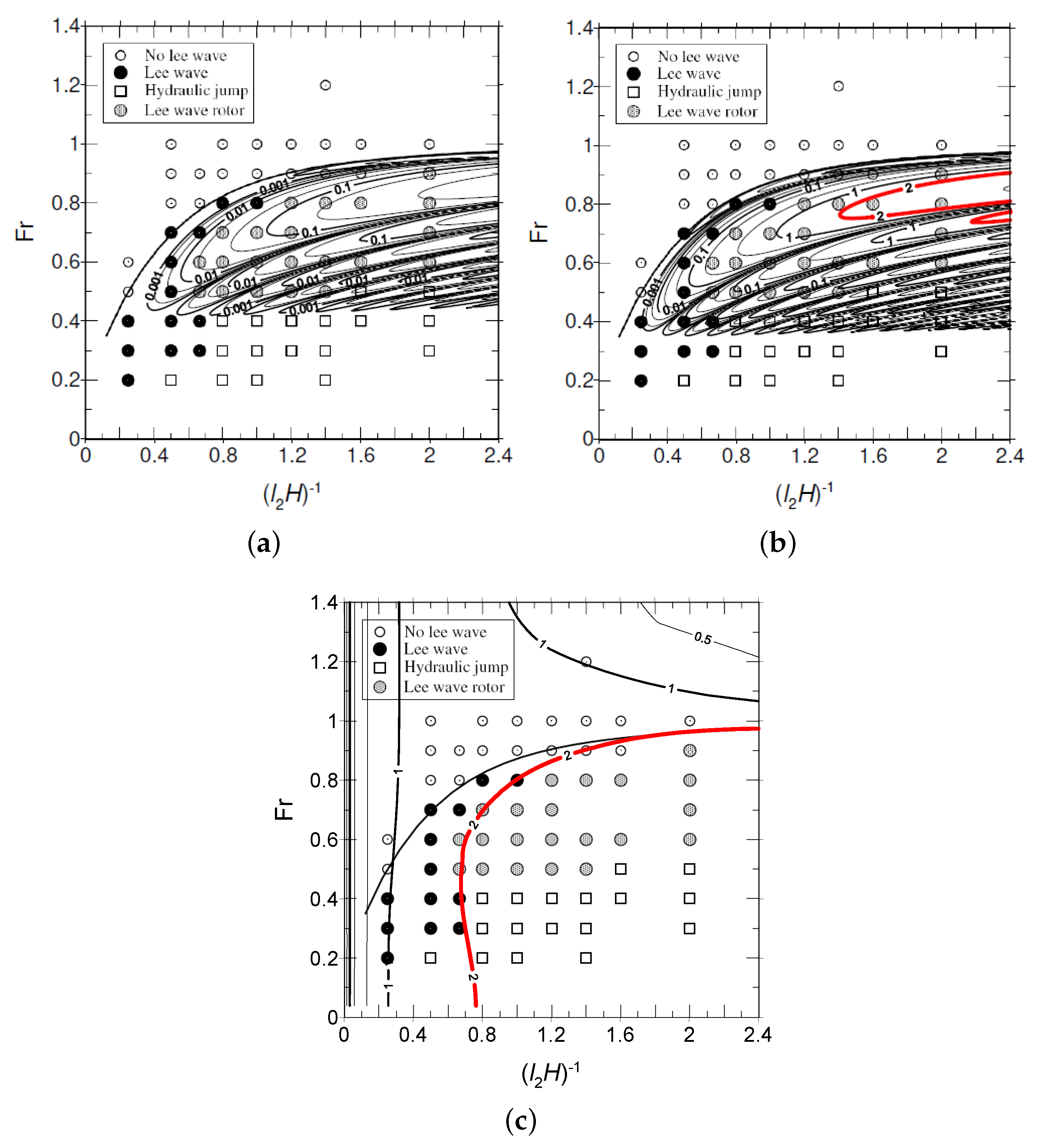
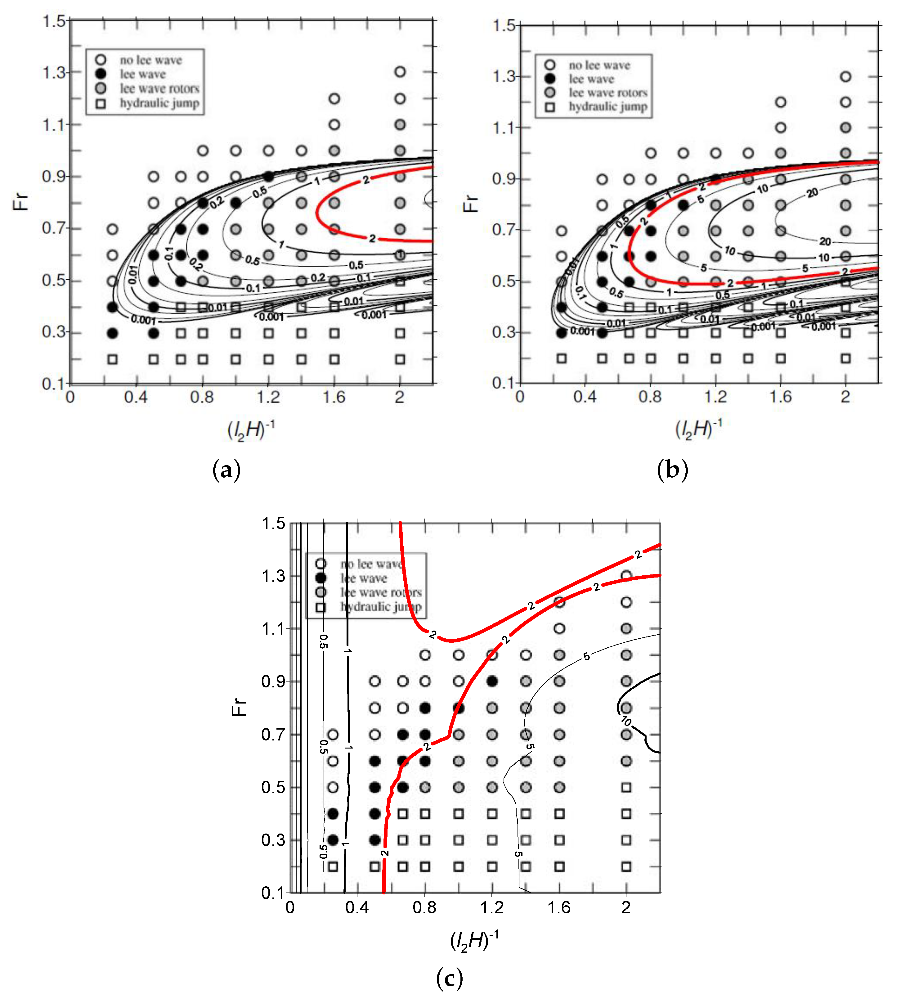
Figure 1 shows ${\left[{\left(l_2{h}_0\right)}_{\mathrm{crit}}\right]}^{-1}$ as a function of ${\left(l_{2}H\right)}^{-1}$ and $Fr$, superposed on the regime diagram of V04 (his Figure 9). In accordance with V04, it is assumed that $l_{2}a=12.5$. Note that, due to the fact that $l_2{h}_0=0.5$, the nonlinearity parameter that appears at the bottom horizontal axis in Figure 9 of V04 ($h_0/H$ in the present notation) can be related to $l_{2}H$ through $h_0/H=\left(l_2{h}_0\right)/\left(l_{2}H\right)=0.5/\left(l_{2}H\right)$. Only thus can the linear model presented here be compared with the numerical simulations of V04, since both $Fr$ and ${\left(l_{2}H\right)}^{-1}$ (but not $h_0/H$) are accessible to linear theory (as noted by TAM13).

Figure 1a shows results from the inviscid model expressed by Equation (25), where the critical mountain height for flow stagnation can be expressed in terms of ${\left(l_2{h}_0\right)}_{\mathrm{crit}}$ via mere multiplication of Equation (25) by $l_{2}H$. Although the highest values of ${\left[{\left(l_2{h}_0\right)}_{\mathrm{crit}}\right]}^{-1}$ are located directly over the region where rotors are diagnosed in the regime diagram of V04, the magnitude of this quantity that is necessary for flow stagnation is severely underestimated. Maximum values are just above 0.2, and the contour of two obviously does not appear in the graph.

Figure 1b shows results from the improved model where the effects of the amplification of $u_{\mathrm{B}}$ and attenuation of $U_{\mathrm{B}}$ in the surface layer are taken into account, but no feedback on the outer flow exists (Equation (26)). The results are substantially improved, but the magnitude of ${\left[{\left(l_2{h}_0\right)}_{\mathrm{crit}}\right]}^{-1}$ is still too small to be consistent with the occurrence of rotors in the regime diagram of V04. One of the reasons for this, as pointed out before, is that ${\left[{\left(l_2{h}_0\right)}_{\mathrm{crit}}\right]}^{-1}$ is directly proportional, through Equation (25), to the Fourier transform of the orography at the resonant wavenumber of the trapped lee waves $k_{\mathrm{L}}^{\prime }$ and is thus zero at the points in parameter space where $\widehat{h}\left(k_{\mathrm{L}}^{\prime }\right)=0$. As the Fourier transform of Equation (28) has several zeros (at $ak/\left(2\pi \right)=n$, where n is an integer; see Figure 14 of V04 and Equation (29) of TAM13), the oblique troughs that can be observed in the contours in Figure 1a,b result from these zeros.

Figure 1c shows the results from the full model, including the effect of the boundary layer on the outer flow, in addition to the direct boundary layer effects described above, and also including the contribution to flow stagnation of waves propagating vertically or evanescent in the upper layer in addition to trapped lee waves. It can be seen that the region of parameter space where ${\left[{\left(l_2{h}_0\right)}_{\mathrm{crit}}\right]}^{-1}>2$ encompasses almost perfectly the region with rotors in the regime diagram of V04. However, it also includes most of the region where a hydraulic jump was observed to occur in those numerical simulations. Figure 8b of KEPE10 shows that at least some types of hydraulic jumps are characterized by localized flow stagnation on the lee slope of the orography, although this does not seem to occur in the case illustrated by Figure 8 of V04. On the other hand, Sachsperger et al. [21] recently noted that hydraulic jumps may be a source of trapped lee waves (which are a prerequisite for rotors). This idea seems to be supported also by the inviscid results presented in Figure 7 of V04. It would be useful to develop a procedure to discriminate between rotors and hydraulic jumps in the present model, but that is beyond the scope of this study.

An interpretation of the behaviour of the flow stagnation condition in the regime diagrams may be facilitated by plotting the velocity perturbation associated with these flows. This only needs to be done for the model that produced the results of Figure 1c, as the models that produced the results of Figure 1a,b assume by design a train of sinusoidal waves downstream of the orography (since they only take into account the trapped lee wave component of the flow). Figure 2 presents $u/U$ and $u_{\mathrm{B}}/U_{\mathrm{B}}$ (the normalized streamwise velocity perturbations outside and inside the surface layer, respectively) from the present model, for the cases analysed in more detail by V04. It should be noted that $u/U=-1$ and $u_{\mathrm{B}}/U_{\mathrm{B}}=-1$ correspond to flow stagnation outside and inside the surface layer, respectively.

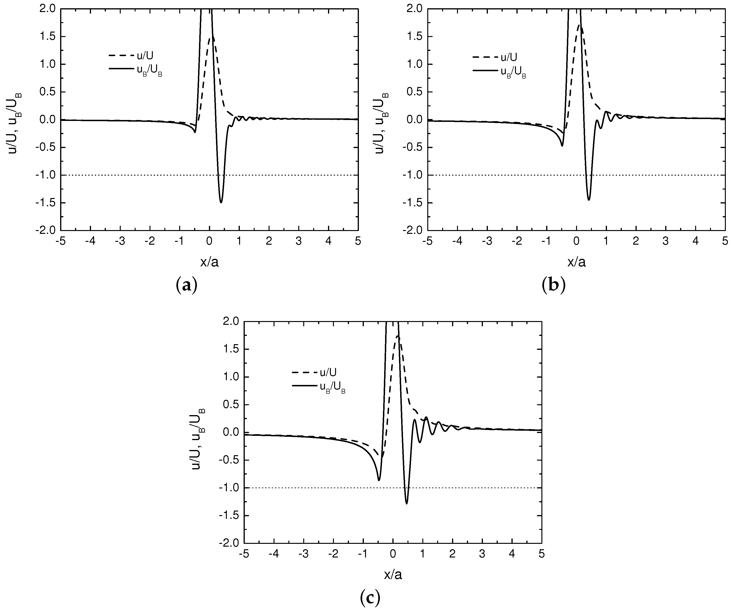
The results in Figure 2a were calculated for $Fr=0.6$ and ${\left(l_{2}H\right)}^{-1}=0.5$, corresponding, according to V04, to a situation with trapped lee waves (although of relatively modest amplitude, at least in terms of their streamwise velocity perturbation; see their Figure 4), but no rotors. It can be seen that both outside and inside the surface layer, the velocity perturbation displays a maximum (much amplified for $u_{\mathrm{B}}/U_{\mathrm{B}}$ with respect to $u/U$), centred roughly over the hill. Inside the surface layer, where this maximum is slightly displaced upstream, it is followed by a minimum downstream of the hill, but no stagnation is produced anywhere.

Figure 2b shows results for the situation with $Fr=0.6$ and ${\left(l_{2}H\right)}^{-1}=1$, which according to V04 corresponds to a case with rotors, displayed in his Figure 5. While in that figure, there is a very strong acceleration of the flow near the ground downstream of the hill and a very pronounced pattern of trapped lee waves with several stagnation points near the surface, the flow pattern from the present model is quite different. Essentially, the velocity perturbation behaves qualitatively similarly to that in Figure 2a, but with a larger amplitude, with amplification of the maximum over the hill and intensification of the downstream minimum, which now is sufficient to induce flow stagnation inside the surface layer, but only once. $u_{\mathrm{B}}/U_{\mathrm{B}}$ shows a very weak trapped lee wave oscillation, which is consistent with the weakness of this flow component inferred from the inviscid results of Figure 1a,b.

This suggests that the trapped lee wave shown in Figure 5 of V04 is highly nonlinear and not directly forced by the orography, unlike assumed in the present model. The relatively modest effect of the surface layer on the outer flow appears to be insufficient to force such a wave. However, it must be recognized that the behaviour of $u_{\mathrm{B}}/U_{\mathrm{B}}$ in the present model makes sense physically: the flow deceleration zone downstream of the hill is due to the effect of friction, corresponding to an incipient flow separation bubble. An upstream migration of the velocity perturbation maximum and a deepening of the velocity perturbation minimum downstream of the hill (which are attenuated, but qualitatively similar, versions of the processes produced by the present model) can be seen, for example, in Figure 3 of Smith [19] or Figure 5 of Jiang et al. [22]. It might be argued that although the present model does not faithfully reproduce the flow structure produced by the numerical simulations directly, the flow stagnation it predicts might act as an indirect trigger for the trapped lee waves and, hence, for the rotors.

Figure 2c shows model results for $Fr=0.4$ and ${\left(l_{2}H\right)}^{-1}=1$, which in V04 corresponds to a situation with a hydraulic jump (his Figure 8). The model results differ relatively little from those displayed in Figure 2b, but substantially from those of V04. The maximum in the velocity perturbation over the hill has decreased relative to Figure 2b, but the minimum remains equally low, corresponding to flow stagnation. The very weak trapped lee wave pattern that was barely discernible in Figure 2b is now absent. This contrasts with the strong downslope wind that can be found near the surface in the numerical simulations. Note, however, that downstream of the hydraulic jump, the flow almost stagnates in those simulations, and the same happens a short distance above the top of the hill.

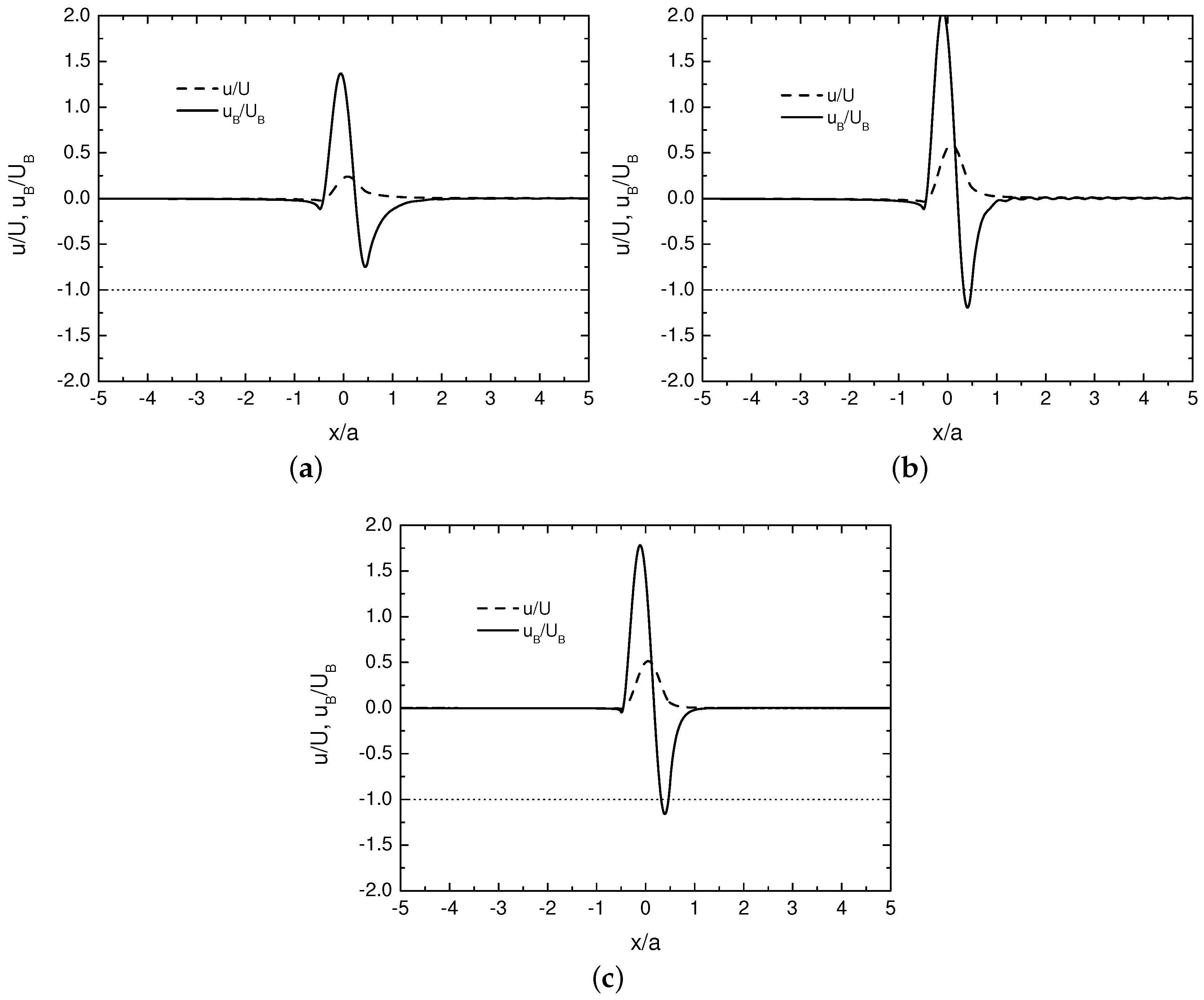
The cases analysed in detail by V04, mentioned above, are rather close to the threshold conditions for the occurrence of rotors in parameter space. Figure 3 shows results where flow stagnation is fulfilled by a wider margin, at least according to the present model.

In Figure 3, it is assumed that ${\left(l_{2}H\right)}^{-1}=2$. In Figure 3a, $Fr=0.7$; in Figure 3b, $Fr=0.8$; and in Figure 3c, $Fr=0.9$. Perhaps the main difference relative to the results presented in Figure 2 is that the maximum of the velocity perturbation over the hill is substantially increased, both outside and inside the surface layer, and the minimum downstream of the hill is also more pronounced. Additionally, there is a clearly noticeable (though spatially attenuated) trapped lee wave signature downstream of the hill (detectable only in $u_{\mathrm{B}}/U_{\mathrm{B}}$) and also a minimum of the velocity perturbation upstream of the hill. Both of these features are especially salient in Figure 3b, for $Fr=0.8$. However, in all cases (as in Figure 2), the signature of non-trapped waves (with velocity perturbations confined to the vicinity of the hill) are largely dominant with respect to the signature of trapped lee waves.

3.3. Numerical Simulations of Sheridan and Vosper (2006)

SV06 performed numerical simulations essentially similar to those of V04, except that $l_{2}a=3.125$ (i.e., more non-hydrostatic flow) was assumed, to produce an analogous regime diagram (their Figure 4). ${\left[{\left(l_2{h}_0\right)}_{\mathrm{crit}}\right]}^{-1}$ calculated from the present model is superimposed on this regime diagram in Figure 4. As in Figure 1, Figure 4a corresponds to results from the inviscid model given by Equation (25), Figure 4b to the improved model given by Equation (26) and Figure 4c to the full model.

In this case, Equation (25) still underestimates very substantially the region of parameter space where ${\left[{\left(l_2{h}_0\right)}_{\mathrm{crit}}\right]}^{-1}$ is larger than two, but the contour of two appears in the graph, as that quantity slightly exceeds this value (see Figure 4a). The improved model (Equation (26)) does a reasonably good job of predicting the region of parameter space where rotors occur (Figure 4b), but slightly underestimates its range, especially for the lowest and highest values of $Fr$. This better agreement than in Figure 1b occurs largely due to the fortuitous fact that the region where flow stagnation is more likely corresponds to trapped lee wave resonant wavenumbers that do not coincide with the zeros of the Fourier transform of $\widehat{h}$. Mathematically, the reason for this is the following: the dimensionless resonant wavenumber $k_{\mathrm{L}}^{\prime }=k_{\mathrm{L}}H$ is only a function of $l_{2}H$ and $Fr$ (not $l_{2}a$) (see Equation (22) of TAM13). Hence, it takes the same values as in V04. However, this wavenumber, as it enters in Equation (28), is normalized instead by a. This means that $k_{\mathrm{L}}a=k_{\mathrm{L}}^{\prime }(a/H)=k_{\mathrm{L}}^{\prime }\left(l_{2}a\right)/\left(l_{2}H\right)$ is smaller in SV06, being centred in a part of the normalized Fourier transform of Equation (28) mostly to the left of the existing zeros (cf. Figure 14 of V04). What this means physically is simply that the forcing a narrower hill provides at the resonant wavenumbers (which tend to be short) is stronger than the forcing provided at the same wavenumbers by a wider hill.

Figure 4c shows results from the full model, where it can be seen that the region of parameter space where ${\left[{\left(l_2{h}_0\right)}_{\mathrm{crit}}\right]}^{-1}>2$ encompasses all cases with rotors observed in the numerical simulations, as well as most of the cases with hydraulic jumps (as in the situation with $l_{2}a=12.5$). The agreement is, however, not as good as in Figure 1, since this region includes some cases classified by SV06 as simply corresponding to trapped lee waves (without rotors) or even no trapped lee waves, particularly for the highest values of $Fr$. The extent of the region of parameter space where flow stagnation is detected in the numerical simulations appears to be slightly overestimated by the full model, although it is impossible to check whether the separate region with the highest values of $Fr$, at the top of the graph, is correct, due to the lack of simulations covering that part of the parameter space.

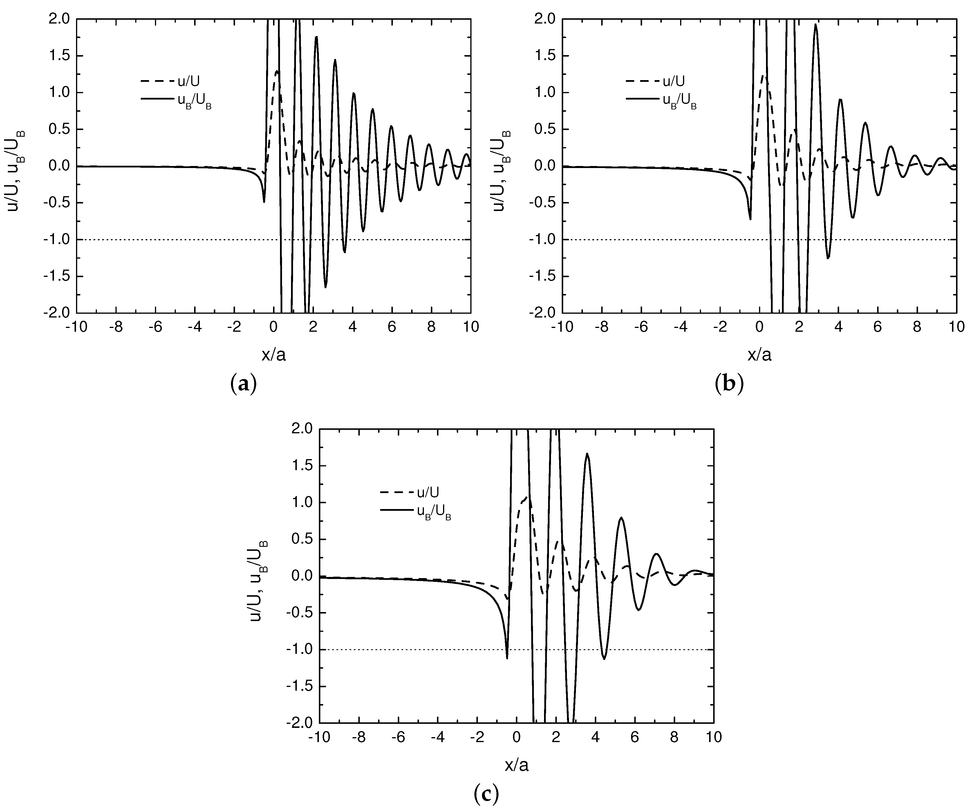
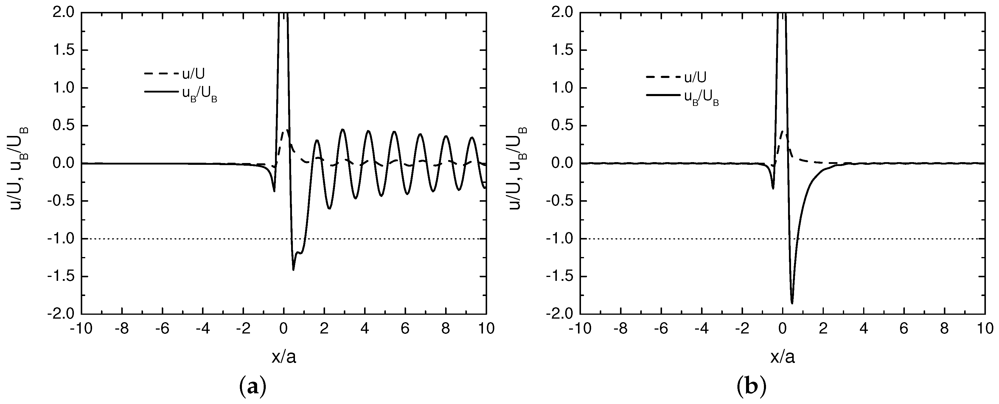
Figure 5 shows the structure of the normalized velocity perturbation in the downstream direction outside and inside the surface layer. SV06 only analyse in more detail two idealized cases: one dominated by rotors, with $Fr=0.6$ and ${\left(l_{2}H\right)}^{-1}=1$ (their Figure 3a) and another one dominated by a hydraulic jump, with $Fr=0.4$ and ${\left(l_{2}H\right)}^{-1}=1$ (their Figure 3b). Figure 5a,b shows the flow perturbations associated with each of these two cases, respectively, obtained from the present model.

Clearly, in Figure 5a, there is a strong signature of trapped lee waves (especially inside, but also outside, the surface layer). In this sense the model behaviour differs from that displayed in Figure 2b, but is consistent with the behaviour of the inviscid and improved models in Figure 4. The trapped lee waves are weaker than those displayed in Figure 3a of SV06, since flow stagnation only occurs at the first trough (which seems to be intensified by a non-trapped wave component). Nevertheless, the wavelength is not too different (though slightly smaller) than that seen in Figure 3a of SV06, being roughly $\lambda /a\approx 1.33$, or equivalently $\lambda \approx 3.33\mathrm{km}$, against $\lambda /a\approx 1.6$, or $\lambda \approx 4\mathrm{km}$ from SV06. In contrast, in Figure 5b, corresponding in SV06 to a hydraulic jump, there is a total absence of trapped lee waves and only one stagnation zone downstream of the orography, much as happened in Figure 1b,c. This is not consistent with the behaviour of the flow perturbation near the ground in the numerical simulations, where Figure 3b of SV06 shows considerable flow acceleration downstream of the mountain, but is perhaps more consistent with the flow higher up, slightly above the top of the hill.

As in Figure 3, Figure 6 presents the velocity perturbation predicted by the model for a parameter combination where flow stagnation is predicted to be fulfilled by a wider margin. The values of $Fr$ and ${\left(l_{2}H\right)}^{-1}$ are the same assumed in Figure 3. In these cases, there is an overwhelmingly dominant trapped lee wave pattern within the surface layer, leading to flow stagnation in three separate regions downstream of the hill. Therefore, these are cases where the model actually predicts rotors, as usually understood, not just flow stagnation. Interestingly, the flow outside the surface layer never approaches stagnation, showing relatively low nonlinearity (as predicted by the model), in contrast with the strong amplification it undergoes within the surface layer. The wavelength of the trapped lee waves increases from Figure 6a–c, as this is a strong function of $Fr$, and increases as $Fr$ increases (see Figure 8 of TAM13). In Figure 6c, for $Fr=0.9$, the model predicts that flow stagnation occurs even upstream of the hill inside the surface layer.

The main conclusion to take from the above results is that, despite the fact that not only the regime diagram presented by SV06, but also the flow structure associated with rotors and hydraulic jumps bear a strong resemblance to the equivalent results produced by V04, they are much more directly forced by the orography in the former case than in the latter. This is demonstrated by the fact that the present model is able to reproduce the flow structure with greater accuracy and that the improved version of the inviscid model is much more consistent with the regime diagram of SV06 than with that of V04.

3.4. Laboratory Experiments of Knigge et al. (2010)

Finally, KEPE10 considered even more non-hydrostatic and nonlinear flows in their laboratory experiments. In the cases treated by them, it is not possible to obtain figures akin to Figure 1 or Figure 4, where uniformly valid results from the present model are superposed on a regime diagram, their Figure 9. Although, as in V04 and SV06, the variable $h_0/H$ on the horizontal axis of that figure can be related to a parameter that is accessible to linear theory, i.e., $a/H=(h_0/H)/(h_0/a)$, where $h_0/a=0.57$ is fixed in the experiments, the value of $l_{2}a$ is not provided for each data point in the regime diagram. Hence, comparisons must be limited to the particular cases analysed in more detail by these authors (their Figures 4–8), where all flow parameters are specified.

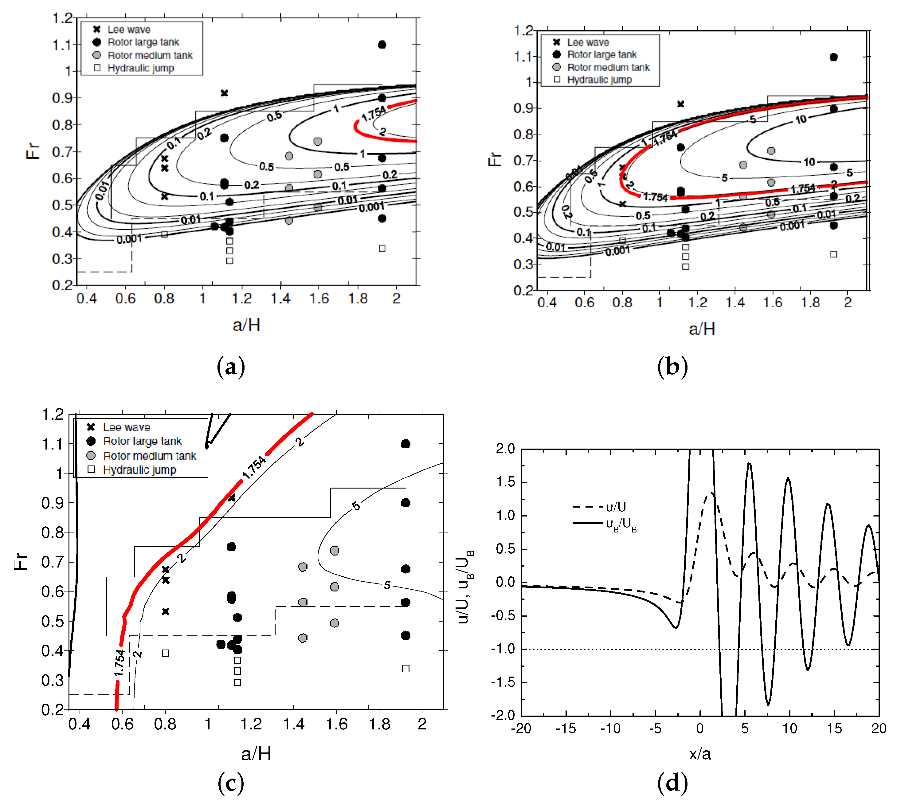
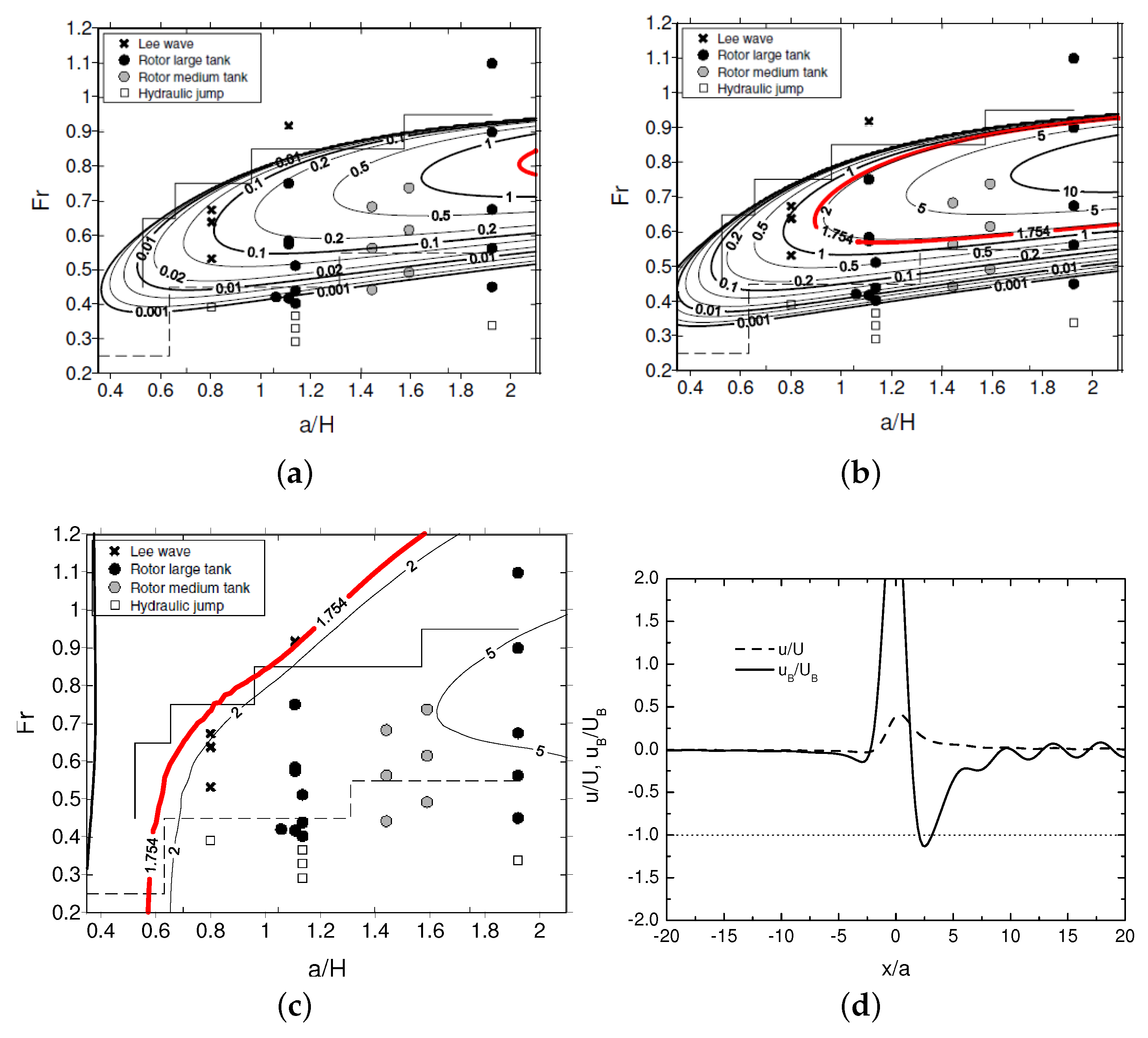
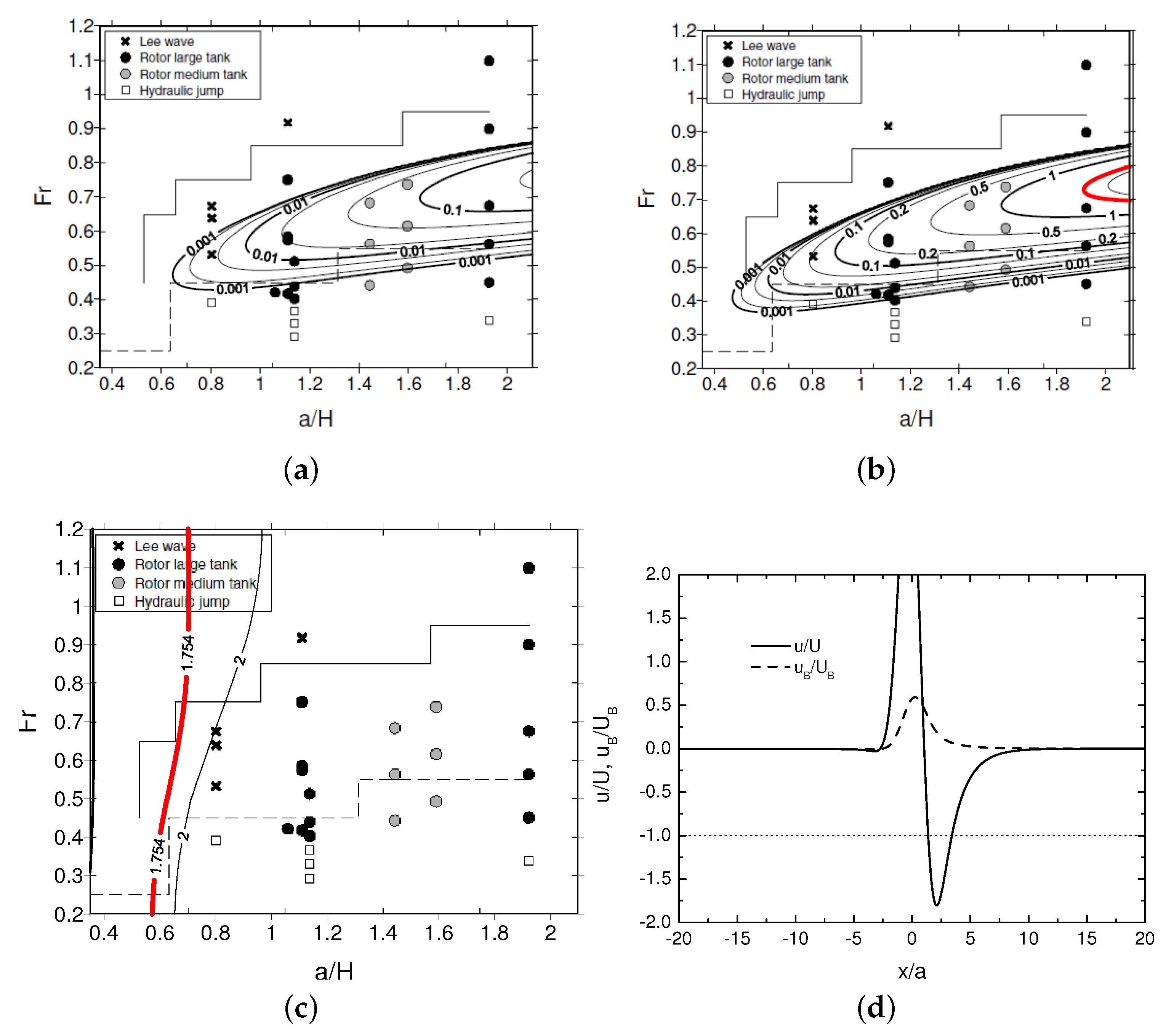
Figure 7 shows results for the case displayed in Figures 4a and 5a of KEPE10, where $l_{2}a=1.426$ (derived from their data as $l_{2}a=\left(l_2{h}_0\right)/(h_0/a)$, given that the inverse of the internal Froude number used by them was $l_2{h}_0=1/1.23$ and $h_0/a=0.57$), $Fr=0.64$ and $a/H=0.807$ (also derived from their data via $a/H=(h_0/H)/(h_0/a)$, with $h_0/H=0.46$).

Note that, unlike in Figure 1 and Figure 4, results from the present model superimposed on the regime diagrams in Figure 7a–c are only valid for the specific conditions quoted above, not for the full range of $a/H$ and $Fr$. Hence, the essential information contained in the contour plots overlaid on the regime diagrams is whether the point corresponding to those conditions is enclosed by contours where flow stagnation is predicted or not. Figure 7a shows results from the inviscid model, Figure 7b from the improved model and Figure 7c from the full model. Figure 7d shows the velocity perturbation derived from the full model, for the same specific conditions.

In Figure 7, it can be seen that both the inviscid and the improved model do not diagnose any flow stagnation, which is consistent with the absence of rotors reported by KEPE10 in this case. The full model, however, marginally predicts flow stagnation, as shown by the fact that the region of parameter space enclosed by the contour of 1.754 contains the point with $a/H=0.807$ and $Fr=0.64$, albeit at its edge. This is confirmed by the fact that in Figure 7d, the flow perturbation minimum just exceeds the stagnation limit. The trapped lee waves that can be detected in $u_{\mathrm{B}}/U_{\mathrm{B}}$ are, however, of relatively low amplitude.

Figure 8 shows similar results, but for the case displayed in Figures 4b, 5b, 6 and 7 of KEPE10, where trapped lee wave rotors were detected. The parameters that can be derived in the same way as described above from their data now take the values: $l_{2}a=1.271$, $Fr=0.9$ and $a/H=1.93$. In this case, all versions of the model except the inviscid one (Figure 8a) diagnose the occurrence of flow stagnation, although for the improved model (Figure 8b), this occurs by a relatively small margin. Stagnation is exceeded more significantly in the full model (Figure 8c), as shown by the fact that the point $Fr=0.9$ and $a/H=1.93$ lies well within the contour of 1.754. The flow perturbation is also dominated by a high-amplitude trapped lee wave signature (Figure 8d), with three zones downstream of the orography where the flow stagnates.

Finally, in Figure 9, the case displayed in Figure 8 of KEPE10 is analysed, where $l_{2}a=2.278$, $Fr=0.37$ and $a/H=1.14$, and a hydraulic jump was detected in the laboratory experiments. Both the inviscid and the improved model do not predict flow stagnation (Figure 9a,b), but the full model (Figure 9c) predicts it, again by a wide margin. However, the velocity perturbation (Figure 9d) does not show any trapped lee wave signature, but rather flow stagnation is achieved as a single zone of flow deceleration that must be caused by non-trapped waves.

The main conclusion to draw from these results is that rotors appear to be, also in this case directly, rather than indirectly, forced, and the full model appears to slightly overestimate the conditions for flow stagnation. However, the comparison of a linear model with these experiments is perhaps more questionable than in the preceding cases, since the laboratory experiments of KEPE10 depart substantially more from the assumptions of linear theory than the numerical simulations of V04 and SV06. Namely, the nonlinearity is stronger ($h_0/a=0.57$ and $l_2{h}_0=0.81,0.72,1.30$, against $h_0/a=0.04$ and $l_2{h}_0=0.5$ in V04 and $h_0/a=0.16$ and $l_2{h}_0=0.5$ in SV06). Additionally, the inversion is thicker (in relative terms) than in the numerical simulations; the velocity boundary layer is thinner and less in equilibrium (since it is only generated by the leading edge of the obstacle); reflection of propagating mountain waves in the layer further away from the hill could not be totally prevented; and the flow structures were diagnosed subjectively (see KEPE10).

Nevertheless, it is remarkable that, even in these far-from-ideal conditions, the fields of ${\left[{(h_0/a)}_{\mathrm{crit}}\right]}^{-1}$ presented in Figure 7, Figure 8 and Figure 9 still show shapes consistent with the zones in parameter space where different types of flow structures are detected. The contours of this quantity in Figure 7b, Figure 8b and Figure 9b display roughly the same shape as the region in parameter space with rotors, and in Figure 7c and Figure 8c, the contours roughly follow the regions of parameter space containing rotors or hydraulic jumps.

4. Conclusions

A model has been developed to predict flow stagnation associated with rotors produced by trapped lee waves in a way that is computationally inexpensive and affords maximum physical insight into the flow behaviour. This was done by coupling the inviscid trapped lee wave model of TAM13 with the bulk boundary layer model of SJD06. The inviscid model of TAM13 considers an atmosphere with constant wind and a neutrally-stratified layer near the surface, topped by a sharp temperature inversion, above which the static stability is constant, an idealized atmosphere adopted by a number of previous authors (V04, SV06, KEPE10). The boundary layer model of SJD06 is essentially a model for representing friction associated with wind shear within the atmospheric surface layer.

The onset of rotors is predicted based on the flow stagnation condition, i.e., that the streamwise velocity component becomes zero. This condition is necessary, but not sufficient, for the existence of rotors. Three versions of the model, with an increasing degree of complexity, are tested. The first one excludes all frictional effects, and flow stagnation is diagnosed from the (analytic) expression for the streamwise velocity component, assuming that only the trapped lee waves are important for this process. In the second version of the model, the flow stagnation condition is corrected for the attenuation of the mean wind and amplification of the flow perturbation within the surface layer. Finally, the full model accounts additionally for feedback of the boundary layer on the outer flow, through a modified surface boundary condition, and for the contribution to flow stagnation given by non-trapped waves. The solution can then only be obtained numerically.

These models were tested against data from the numerical simulations of V04 and SV06 and the laboratory experiments of KEPE10. The main conclusions are the following: when adequately calibrated, both the improved inviscid model and the full model have some ability to predict rotors as corresponding to the regions of parameter space where the flow stagnation condition is fulfilled or exceeded. While the improved model underestimates the occurrence of rotors in the more hydrostatic case treated by V04, it is able to diagnose them in an essentially correct way in the more non-hydrostatic cases treated by SV06 and KEPE10. On the other hand, the full model, via a more complete treatment of frictional effects, is able to predict fairly well the occurrence of both rotors and hydraulic jumps in all cases considered here, although the flow stagnation condition is unable to discriminate between these two flow structures and appears to slightly overestimate the occurrence of flow stagnation in the more non-hydrostatic cases of SV06 and KEPE10. However, the velocity perturbations obtained from the full model clearly show that flow stagnation in situations characterized by previous authors as having hydraulic jumps is not associated with any trapped lee waves, being caused instead (at least in the model) by non-trapped waves. This could form the basis of a methodology to discriminate between rotors and hydraulic jumps, but that is beyond the scope of the present contribution.

The flow structure calculated from the full model shows that, although this version of the model apparently can be calibrated to produce good results, the physical reasons for flow stagnation appear not to be always correct, especially for hydraulic jumps and for the rotor cases treated by V04. In V04’s numerical simulations, this turns out to be due to the rather fortuitous fact that the direct forcing of trapped lee waves by the orography is very weak, owing to the existence of zeros in the Fourier transform of the surface elevation chosen by him. In these numerical simulations, the trapped lee waves appear to be indirectly generated by nonlinear processes (as pointed out originally by V04), since the linear model, despite being able to produce flow stagnation in the correct regions of parameter space when frictional effects are included, does not produce it for the right reasons. The model shows the potential to perform globally better for orographies whose Fourier transforms do not have zeros (as happens in the laboratory experiments of KEPE10) or when the resonant wavelength of the trapped lee waves does not coincide with these zeros (as in SV06). In those cases, the present study suggests that even the improved inviscid model could have substantial predictive power.

The input parameters of the surface layer model adopted here take values selected among an ample range of suitable choices and cannot be considered definitive. It is possible that the model performance could still be optimized further by adopting a different set of values.

References

1. Kuettner, J.; Hertenstein, R.F. Observations of mountain-induced rotors and related hypotheses: A review. In Proceedings of the 10th Conference on Mountain Meteorology, Park City, UT, USA, 17–21 June 2002; pp. 326–329.
2. Darby, L.S.; Poulos, G.S. The evolution of lee-wave-rotor activity in the lee of Pike’s Peak under the influence of a cold frontal passage: Implications for aircraft safety. Mon. Weather Rev. 2006, 134, 2857–2876. [Google Scholar] [CrossRef]
3. Agustsson, H.; Ólafsson, H. Simulations of observed lee waves and rotor turbulence. Mon. Weather Rev. 2014, 142, 832–849. [Google Scholar] [CrossRef]
4. Doyle, J.D.; Durran, D.R. Rotor and subrotor dynamics in the lee of three-dimensional terrain. J. Atmos. Sci. 2007, 64, 4202–4221. [Google Scholar] [CrossRef]
5. Hertenstein, R.F. The influence of inversions on rotors. Mon. Weather Rev. 2009, 137, 433–446. [Google Scholar] [CrossRef]
6. Smith, C.M.; Skyllingstad, E.D. Investigation of upstream boundary layer influence on mountain wave breaking and lee wave rotors using a large-eddy simulation. J. Atmos. Sci. 2009, 66, 3147–3164. [Google Scholar] [CrossRef]
7. Doyle, J.D.; Durran, D.R. The dynamics of mountain-wave-induced rotors. J. Atmos. Sci. 2002, 59, 186–201. [Google Scholar] [CrossRef]
8. Vosper, S.B. Inversion effects on mountain lee waves. Q. J. R. Meteorol. Soc. 2004, 130, 1723–1748. [Google Scholar] [CrossRef]
9. Belcher, S.E.; Harman, I.N.; Finnigan, J.J. The wind in the willows: Flows in forest canopies in complex terrain. Ann. Rev. Fluid Mech. 2012, 44, 479–504. [Google Scholar] [CrossRef]
10. Belcher, S.E.; Hunt, J.C.R. Turbulent flow over hills and waves. Ann. Rev. Fluid Mech. 1998, 39, 507–538. [Google Scholar] [CrossRef]
11. Smith, R.B. Mountain-induced stagnation points in hydrostatic flow. Tellus 1989, 41A, 270–274. [Google Scholar] [CrossRef]
12. Teixeira, M.A.C.; Argaín, J.L.; Miranda, P.M.A. Orographic drag associated with lee waves trapped at an inversion. J. Atmos. Sci. 2013, 70, 2930–2947. [Google Scholar] [CrossRef]
13. Vosper, S.B.; Sheridan, P.F.; Brown, A.R. Flow separation and rotor formation beneath two-dimensional trapped lee waves. Q. J. R. Meteorol. Soc. 2006, 132, 2415–2438. [Google Scholar] [CrossRef]
14. Smith, R.B.; Jiang, Q.; Doyle, J.D. A theory of gravity wave absorption by a boundary layer. J. Atmos. Sci. 2006, 63, 774–781. [Google Scholar] [CrossRef]
15. Hunt, J.C.; Leibovich, S.; Richards, K.J. Turbulent shear flows over low hills. Q. J. R. Meteorol. Soc. 1988, 114, 1435–1470. [Google Scholar] [CrossRef]
16. Scorer, R.S. Theory of waves in the lee of mountains. Q. J. R. Meteorol. Soc. 1949, 75, 41–56. [Google Scholar] [CrossRef]
17. Sheridan, P.F.; Vosper, S.B. A flow regime diagram for forecasting lee waves, rotors and downslope winds. Meteorol. Appl. 2006, 13, 179–195. [Google Scholar] [CrossRef]
18. Knigge, C.; Etling, D.; Paci, A.; Eiff, O. Laboratory experiments on mountain-induced rotors. Q. J. R. Meteorol. Soc. 2010, 136, 442–450. [Google Scholar] [CrossRef]
19. Smith, R.B. Interacting mountain waves and boundary layers. J. Atmos. Sci. 2007, 64, 594–607. [Google Scholar] [CrossRef]
20. Eiff, O.S.; Huteau, F.; Tolu, J. High-Reynolds number orographic wave-breaking experiments. Dyn. Atmos. Oceans 2005, 40, 71–89. [Google Scholar] [CrossRef]
21. Sachsperger, J.; Serafin, S.; Grubisic, V.; Stiperski, I.; Paci, A. The amplitude of lee waves on the boundary-layer inversion. Q. J. R. Meteorol. Soc. 2016, in press. [Google Scholar] [CrossRef]
22. Jiang, Q.; Smith, R.B.; Doyle, J.D. Impact of the atmospheric boundary layer on mountain waves. J. Atmos. Sci. 2008, 65, 592–608. [Google Scholar] [CrossRef]
Figure 1. Inverse of the critical dimensionless mountain height [ ( l 2 h 0 ) crit ] 1 as a function ( l 2 H ) 1 and F r for l 2 a = 12.5 , superposed on V04’s regime diagram (adapted from Figure 9 of V04). Contours: 5, 2, 1, 0.5, 0.2, 0.1, and so on. The contour of two is denoted by a thick red line. (a) Inviscid model Equation (25); (b) improved model Equation (26); (c) full model.
Atmosphere 08 00005 g001
Figure 2. Velocity perturbation normalized by the mean velocity outside ( u / U ) and inside ( u B / U B ) the surface layer (see legend), as a function of downstream distance from the orography (assumed to be centred at x = 0 ) normalized by its width, calculated from the full model for l 2 a = 12.5 . Horizontal dotted line: flow stagnation threshold. (a) F r = 0.6 , ( l 2 H ) 1 = 0.5 ; (b) F r = 0.6 , ( l 2 H ) 1 = 1 ; (c) F r = 0.4 , ( l 2 H ) 1 = 1 .
Atmosphere 08 00005 g002
Figure 3. Similar to Figure 2, except that (a) F r = 0.7 , ( l 2 H ) 1 = 2 ; (b) F r = 0.8 , ( l 2 H ) 1 = 2 ; (c) F r = 0.9 , ( l 2 H ) 1 = 2 .
Atmosphere 08 00005 g003
Figure 4. Similar to Figure 1, except that l 2 a = 3.125 , and the contour plots are superposed on the regime diagram of SV06. Adapted from Figure 4 of SV06.
Atmosphere 08 00005 g004
Figure 5. Similar to Figure 2, except that l 2 a = 3.125 . (a) F r = 0.6 , ( l 2 H ) 1 = 1 ; (b) F r = 0.4 , ( l 2 H ) 1 = 1 .
Atmosphere 08 00005 g005
Figure 6. Similar to Figure 5, except that (a) F r = 0.7 , ( l 2 H ) 1 = 2 ; (b) F r = 0.8 , ( l 2 H ) 1 = 2 ; (c) F r = 0.9 , ( l 2 H ) 1 = 2 .
Atmosphere 08 00005 g006
Figure 7. (ac) Inverse of the critical dimensionless mountain height [ ( h 0 / a ) crit ] 1 as a function of a / H and F r for l 2 a = 1.426 , superposed on KEPE10’s regime diagram (adapted from Figure 9 of KEPE10). Contours: 5, 2, 1, 0.5, 0.2, 0.1, and so on. The contour of 1.754 is denoted by a thick red line. (a) Inviscid model Equation (25); (b) improved model Equation (26); (c) full model; (d) u / U and u B / U B as a function of x / a for l 2 a = 1.426 , F r = 0.64 , a / H = 0.807 .
Atmosphere 08 00005 g007
Figure 8. (ac) Similar to Figure 7a–c, except that l 2 a = 1.271 ; (d) similar to Figure 7d, except that l 2 a = 1.271 , F r = 0.9 , a / H = 1.93 .
Atmosphere 08 00005 g008
Figure 9. (ac) Similar to Figure 8a–c, except that l 2 a = 2.278 ; (d) similar to Figure 8d, except that l 2 a = 2.278 , F r = 0.37 , a / H = 1.14 .
Atmosphere 08 00005 g009