1. Introduction
Global warming and urbanization have severely influenced regional climate and caused many extreme climate events in recent decades [
1], attracting more and more attention.
In the past 100 years, global mean temperature (GMT) has risen about 0.72 °C and the average rising rate (ARR) was 0.072 °C/10 years [
2]. Particularly, in the most recent 50 years, ARR has reached about 0.13 °C/10 years, which is two times the ARR over the last 100 years [
3,
4]. In the next 50 years, GMT will keep rising at the rate of 0.24 °C/10 years [
5]. In addition, the response of regional climate change to global warming has also been proved. Zhang [
6] revealed that from 1961 to 2007, the annual mean temperature has risen about 1.8 °C in arid areas in China and the heating intensity was stronger than global average. After comparing the temperature changing trends (TCT) in China and global in recent 100 years, Wang [
7] indicated that TCT in China was basically the same as northern hemisphere. However, in the recent decades, the warmest and the coldest phase did not appear in the same period.
Meanwhile, with the increasing of human activities, urbanization has become one of the most important factors that influence urban climate change in recent decades. A number of studies have indicated that the impact of urbanization on climate has continuously strengthened in the recent years [
8,
9,
10,
11]. Hua [
12] reported that the impact of urbanization on air temperature has displayed sharp changes since 1978 in China. The cities with strong urban heat island (UHI) effects were mainly located in regions with rapid industrial and economic development. The analysis of the temperature changes revealed that future urbanization will strongly affect minimum temperature, whereas little impact was detected for maximum temperature. The minimum temperature changes will be noticeable throughout the year [
13]. In addition, the changes of land use, such as urban expansion, deforestation and declining area of water bodies, will also influence the intensity and distribution of UHI [
14]. Besides, Motha and Baier [
15] pointed out that warming trend caused by the urbanization was even more than the change of regional climate background. All of the above views can indicate that urbanization has the great impact on urban climate.
As the biggest metropolis in China, Shanghai has most typical urban climate features. One of these features is that TCT in Shanghai is not only influenced by global warming but also impacted by urbanization. Therefore, many scholars have studied the response of TCT in Shanghai to global warming and urbanization. Xu [
16] reported that in recent hundred years, TCT in Shanghai was similar to northern hemisphere and it had obvious features of stages, paroxysmal and periodicity. However, the changing process and amplitude of Shanghai was different from northern hemisphere, especially in the past 20 years. Zhou [
17] revealed that the urbanization of Shanghai had significant influence on city climate. Although this impact could not change the main TCT caused by global climate change, it could widen the temperature gap between urban and rural area. Cao [
18] found that various urban development indicators had significant correlation with the temperature difference between urban and suburban in Shanghai, among which, Shanghai residential construction was the main driving force causing UHI. City population and economic development also had obvious influence.
Our study aimed to find out the temperature change of Shanghai and its response to global warming and urbanization. In order to solve this problem, we firstly put emphasis on comparing temperature changing trend and cycles of Shanghai and global in multiple time scales. Next, we tried to find out their cross correlation by using Mann–Kendall test, Empirical Mode Decomposition, Cross Wavelet analysis and statistical analysis methods so that we can understand the response of TCT in Shanghai to global warming in-depth. Then, we induced a comprehensive index to reflect the urbanization level by using principal component analysis (PCA) method. Based on this index, we analyzed the impact of urbanization on TCT in Shanghai by establishing regression equations. Finally, in order to find out what possible results have global warming and urbanization caused in Shanghai, we took the frequency of annual extreme high (low) temperature (EHT or ELT) events in Shanghai as an example to investigate.
2. Data and Methodology
2.1. Data
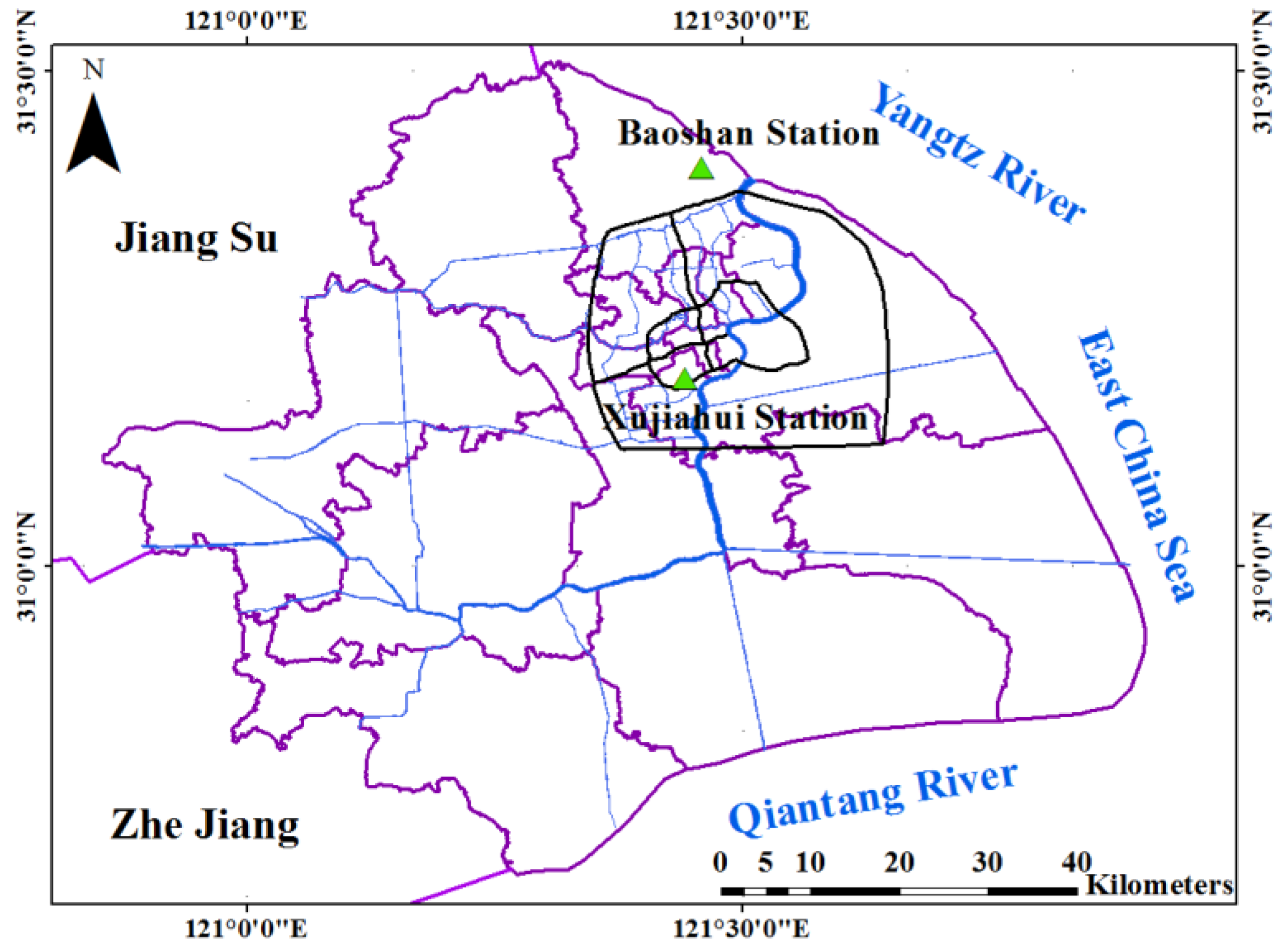
Shanghai (31°14′N, 121°29′E), with 3124 km2 built-up area and over 24 million population, is the most important metropolis in East China. With a typical subtropical monsoon climate, Shanghai has plenty of rainfall and four distinct seasons. The annual mean temperature of Shanghai is about 15 °C and annual mean precipitation is about 1100 mm.
Xujiahui and Baoshan meteorological stations are the only two national meteorological stations in Shanghai. Thus, they have the most detailed long-term meteorological data. Besides, as shown in
Figure 1, Xujiahui meteorological station is located in the city center. The data of Xujiahui station can represent the urban climate. As a comparison, Baoshan meteorological station is located in the typical suburban area. Therefore, the data of Baoshan can accurately reflect the suburban climate. Thus, we selected these two stations as our data source.
To investigate the response of TCT in Shanghai to global warming and urbanization, we used GMT dataset, Shanghai temperature dataset and Shanghai social-economic statistical dataset. GMT dataset, including global annual mean temperature from 1880 to 2015, is available on NOAA's website. Shanghai temperature dataset, including daily mean temperature, maximum temperature and minimum temperature of Xujiahui and Baoshan stations from 1880 to 2015, is provided by China meteorological data website.
Global temperature change (1880 to 2015 from GMT dataset) was caused by both nature and human factors. In order to make our study comparable, the Shanghai annual mean temperature used in this paper was calculated as the annual mean values of the daily mean temperatures of Xujiahui station because temperature data from Xujiahui could be the most typical reflection of the comprehensive influence of nature and human factors in Shanghai.
In addition, Shanghai social-economic statistical dataset, including GDP, population, energy consumption, green space area and urban built-up area, number of vehicles and city farmland area, from 1985 to 2014 was taken from the Shanghai statistical yearbooks.
2.2. Methodology
2.2.1. Mann-Kendall Test
Mann-Kendall test [
19,
20] is widely used to detect significant trends in climatologic time series. Here we used this method to test the trends of global and Shanghai temperature. The calculation steps [
21,
22] are as follows:
(1) For a time series {
xi:
i = 1,2,...,n}, define an order series S
k:
where
(2) Assuming the distribution of time series is random and independent, define statistic UF
k:
where E (S
k) and Var (S
k) are mean and variance of S
k, respectively They can be calculated as follows in the assumption that the distribution of time series
xt is random and independent:
(3) Reserve time series xt: (xn, xn-1, …, x1) and repeat above-mentioned steps. Let UBk = −UFk (k = n, n−1, … , 1), UB1 = 0 and draw the curves of UFk and UBk in the same coordinate system. UFi and UBi follow the normal distribution. If significance testing level α is given, intersection point of the two curves, which is located between the critical lines, indicates the abrupt point. If UFk line is above the upper critical line, it means increasing trend. Else, if UFk line is below the lower critical line, it means decreasing trend.
2.2.2. Maximum Entropy Spectrum Analysis
Maximum Entropy Spectrum (MES) analysis is based on power spectrum and aims to extract the main cycle of a time series. The calculation method is based on Burg algorithm, the principle of which is to establish auto-regression model with proper order and calculate the maximum entropy spectrum [
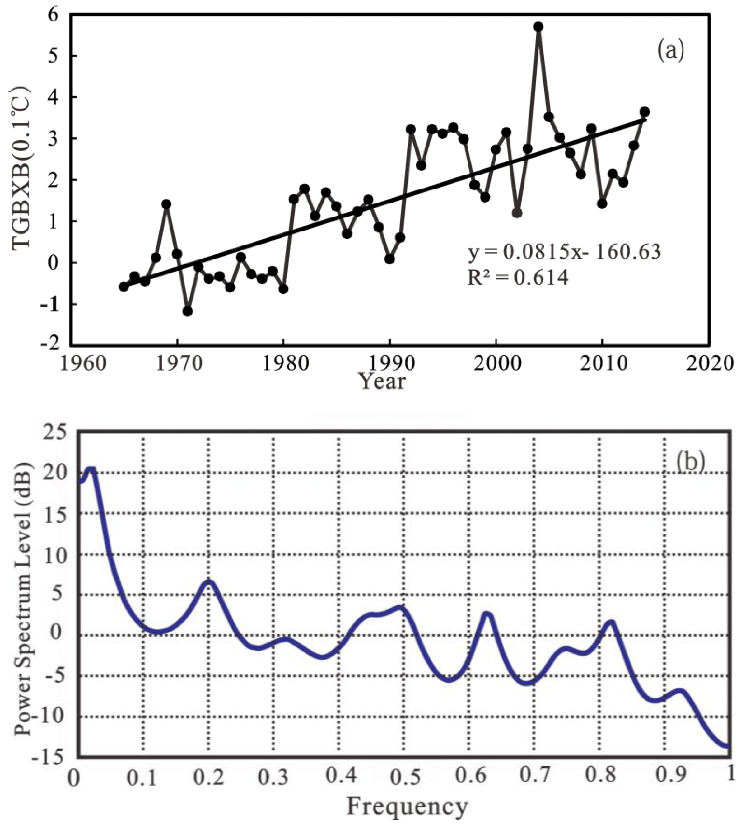
23]. In this study, maximum entropy spectrum analysis was used to calculate the cycle of temperature gap between Xujiahui and Baoshan (TGBXB) in Shanghai.
2.2.3. Empirical Mode Decomposition (EMD)
The EMD, proposed by Huang [
24,
25] in 1998, is a non-stationary signal processing method. It can decompose a signal fluctuations or trends step by step in different scales, and transform the signal into a series of time series with different feature dimensions, which is called the intrinsic mode function (IMF). Among these IMFs, the lowest frequency one can reflect is the overall trend of the original sequence, which is also called the trend term. This paper uses this method to analyze the response of the temperature change in Shanghai to global warming in different time scales.
The calculation steps of EMD are as follows:
- (1)
Calculate all the local limit point of the signal s (t).
- (2)
Evaluate the upper and lower envelope of the signal s (t). Mark upper envelope as u0 (t) and lower envelope as v0 (t).
- (3)
Mark the mean value of upper and lower envelope as m
0 (
t):
and mark the difference value between signal s(
t) and mean value of upper and lower envelope as m
0 (
t) and h
0 (
t):
- (4)
Judge whether h0 (t) satisfies the two properties of IMF. If satisfied, h0 (t) is one of the IMFs; otherwise, mark h0 (t) as s (t), and then repeat Steps 1 to 3 until h0 (t) satisfies the condition of IMF. Finally, mark h0 (t) as c1 (t).
- (5)
Let r1 (t) = s (t) − c1 (t) be a new signal. Then, repeat Steps 1 to 4, thus, getting the second IMF, marked as c2 (t). Next, Let r2 (t) = r1 (t) − c2 (t), and repeat above step, until rn (t) is a monotonous signal or the value of rn (t) is smaller than given threshold. Finally, end the decomposition.
Through the above steps, we can get n IMFs and a residue term.
2.2.4. The Cross Wavelet Analysis
Cross wavelet analysis is a new and effective method to analyze the cross-correlation between two time series, but its application to geological and climatological time-series is still limited [
26]. However, the use of Cross wavelet analysis in many studies have already provided some new insights in the temporal-changing relationships between El Nino, ice condition or tree growth, or magnetic paleointensity and remnant magnetization [
27,
28,
29,
30]. In this study, this method will be applied to analyze the cross-correlation between GMT and Shanghai annual mean temperature.
The calculation steps of Cross Wavelet analysis [
31,
32] are as follows:
The cross wavelet transform of two time series X and Y is defined as:
where
and
are the wavelet coefficient of X, and the complex conjugate of the wavelet coefficient of Y. They can be calculated as follows:
with:
where a and τ are scale and time variables, respectively, and
represents the wavelet family generated by continuous translation and dilation of mother wavelet
. Morlet wavelet was implemented in this study because it is not only a non-orthogonal mother wavelet but also an exponent complex wavelet adjusted by the Gaussian [
33]. In addition, Morlet wavelet also contains more vibration information, the wavelet power can contain positive and negative peak into a wide peak [
33]. Morlet wavelet is defined as:
where ω
0 is a constant, the Morlet wavelet can approach the admissible conditions when ω
0 ≥ 5, its first and second derivative approach zero. It also has good time-frequency resolution [
34]. The wavelet spectrum
of x (
t) is defined as the modulus of its wavelet coefficients:
where
and
are the wavelet coefficient.
2.2.5. Fast Fourier Transform (FFT)
Fast Fourier transform (FFT) was put forward by Cooley and Tukey [
35] in 1965. They took advantage of WN factor’s symmetry and periodic feature, constructing a fast algorithm of DFT, named fast discrete Fourier transform (FFT). In recent decades, FFT algorithm has been further developed [
36]. In this paper, we will use FFT to find the main cycle of each IMF decomposed by EMD method.
The definition of FFT is as follows:
Assuming
is the function of two independent variables
x and
y, and
satisfies the condition that
, then FFT of
is defined as:
Fourier inverse transform is defined as:
Amplitude spectrum, phase spectrum and energy spectrum of Fourier transform are, respectively, defined as:
2.2.6. Extreme Temperature and Its Threshold
Extreme temperature threshold (ETT) is an index used to measure whether the daily maximum (minimum) temperature significantly deviates from average state and can be judged as an extreme event. If the temperature exceeds ETT, we define it as extreme high (low) temperature (event) [
37,
38].
Because of the climatic zone and morphology varies in different areas, the frequency and amplitude of local temperature fluctuation is not the same. Therefore, extreme temperature threshold is different in different areas, so we cannot use a fixed value to describe the ETT. In this paper, we use Bonsal’s method [
39] to get the ETT value for every day in Shanghai. This method does not need the temperature to obey a certain distribution, and it is easy to calculate.
The calculatiion method is as follows:
First, the daily maximum (minimum) temperature should be sorted in ascending (descending) order for the same day from 1960 to 2014.
Second, find the 95th (5th) percentile of the daily maximum (minimum) temperature series and take it as extreme high (low) temperature (EHT (ELT)) threshold, thus, we will get 365 (366) thresholds.
Finally, we take it as an EHT (ELT) event day if daily maximum (minimum) temperature is higher (lower) than EHT (ELT) threshold.
For the determination of extreme event thresholds, we referred to the Bonsal’s method [
39]. If one meteorological element has n values, we sort these values in ascending order:
x1,
x2, …,
xm, …
xn (
x1 ≤
x2 ≤, …, ≤
xm ≤, …≤
xn).
For one value, the probability of not being larger than
xm is
where m is serial number of
xm, and n is total number of meteorological element. If there are 30 values, the 90th percentile was interpolated by the ones of
x27 (P = 87.9%) and
x28 (P = 91.1%) linearly.
2.2.7. The Linear Function for Detecting Transit Jump Point of A Time Series
Linear function for detecting transit jump point of a time series is a new method [
40] for detecting turning points of a time series trend. This method can not only find the turning points, but can also judge whether the turning point can pass the statistical significance test. This paper used this method to find the turning point of annual total number of EHT (ELT) events.
The calculation method is as follows:
Set time sequence Yt = [y1, y2,…, yn], testing steps of finding the turning point of a time series trend is as follows:
(1) Time variable t ∈ [1, n]. Insert n-2 points in (1,n]. Thus, the time variable t is divided into n intervals, marked as (1, 2], (2, 3],..., (n − 1, n].
(2) According to the intervals and half polynomial, establish a new independent variable set. Let:
where
Then, Equation (18) can be turned into linear regression form:
(3) Introduce the stepwise regression technique. Under the condition that the sign of regression coefficients of adjacent independent variables is opposite, screen Zi, and, then, the optimal variables can be automatically selected. We can find the turning points that exist in the time series by analyzing the selected variables.
3. Results
3.1. Temperature Change in Shanghai and Its Response to Global Warming
In this section, we first compared the TCT in Shanghai and globally from 1880 to 2015 by applying regression equations and the Mann-Kendall test. Next, we used the EMD method to compare the temperature cycles in Shanghai and globally over different time scales and then used a cross wavelet analysis to find their cross-correlation. Finally, we established a regression equation between the Shanghai temperature and global temperature to find their interrelationships.
3.1.1. Change Trend Comparison
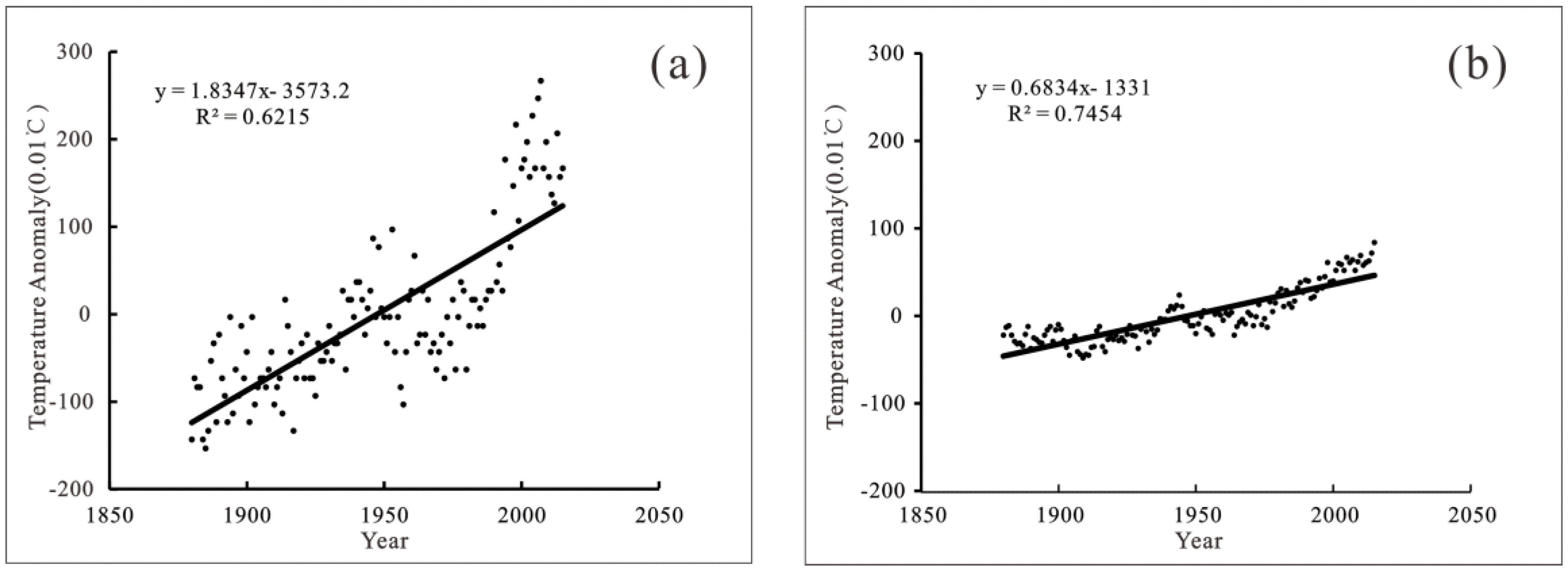
Based on the temperature anomaly data in Shanghai and globally from 1880 to 2015, we established a linear regression equation (
Figure 2) that suggested the temperature anomaly both in Shanghai and globally changed from negative to positive in 1947, indicating that their turning points were in the same year. Additionally, the correlation coefficient (CORRCOEF) of these two time series reached 0.85, which passed the 99.9% confidence test. This result means that the TCT in Shanghai was highly correlated to global warming.
Considering the rate of change in the past 135 years (1880–2015), the ARR of the Shanghai annual mean temperature was about 0.18 °C/10 years, which was more than double the global ARR (0.068 °C/10 years). In the past 50 years, the temperature rose more quickly in Shanghai, with an ARR of 0.56 °C/10 years, which was triple the global rate (0.18 °C/10 years). In addition, the amplitude of the Shanghai annual mean temperature fluctuation was greater than the global fluctuation.
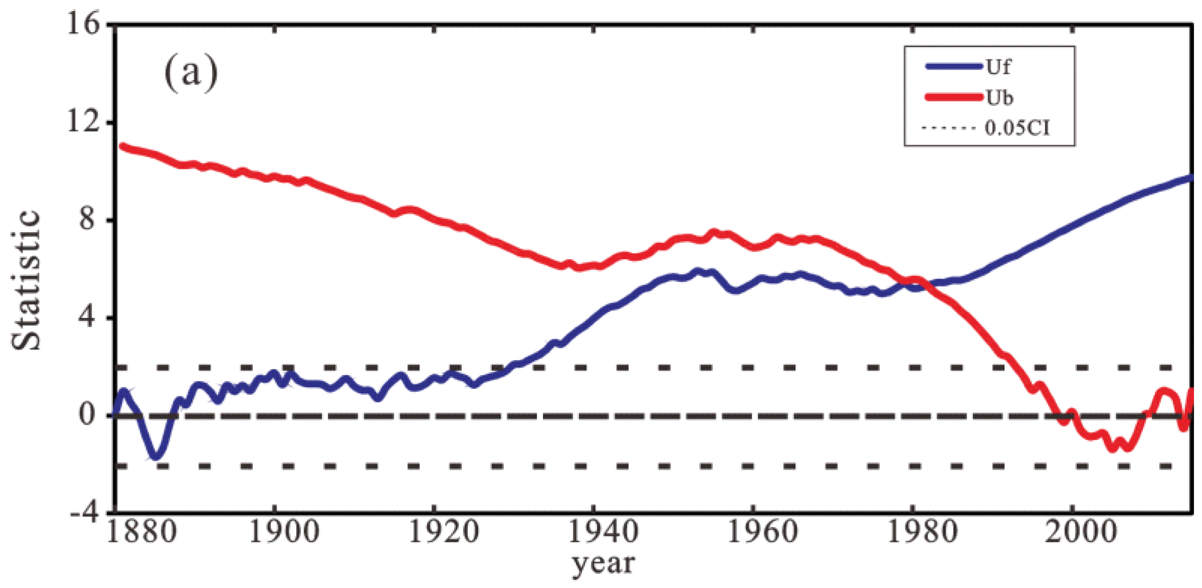
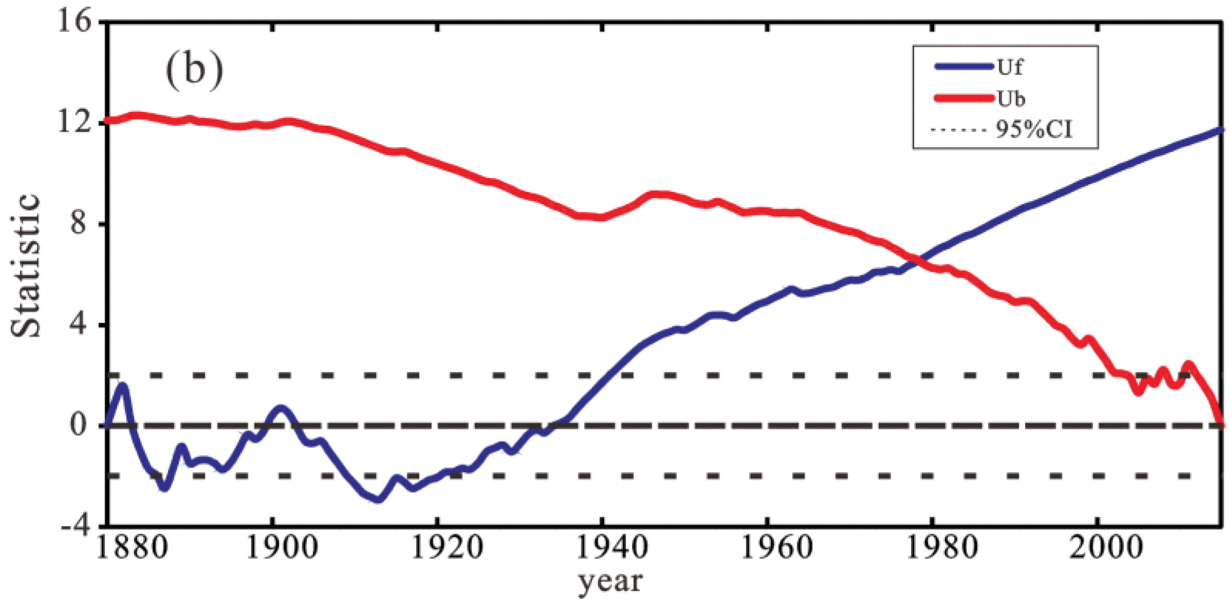
After establishing the linear regression equation, we used the Mann-Kendall test to determine the changing rules between the Shanghai and global mean temperatures. The results of the M-K test had three features:
(1) From 1880 to 1930, the TCT (temperature changing trends) of Shanghai was relatively stable. Under the 0.05 significance level, there was no obvious trend. However, a turning point appeared in 1930 in Shanghai, with a stable increasing trend being established in 1930 and the increasing trend becoming stronger after 1980. By contrast, the GMT showed a significant increasing trend after 1930, which means that its turning point lagged behind that of Shanghai. In addition, the GMT showed stronger fluctuations than that of Shanghai during 1880 to 1940, and it showed a decreasing trend from 1909 to 1920.
(2) The intersection of the UFk and UBk for Shanghai and globally is above 1.96, which means that at the significance level of 0.05, both the Shanghai and global mean temperatures had no abrupt change point from 1880 to 2015. In other words, the Shanghai and global temperature changed smoothly during the past 135 years.
(3) The statistic UF
k in the M-K test is a standardized order series, which can reflect the main trend of the original time series. In
Figure 3, it is obvious that the UF
k series of the Shanghai temperature anomaly was consistent with that of the global temperatures. The CORRCOEF reaches 0.95, which passed 99% confidence test.
3.1.2. Change Cycle Comparison
Section 3.1.1 illustrates that the Shanghai TCT was highly related to global warming. In this section, we mainly focus on comparing the temperature change cycle between the local temperature at Shanghai and the global temperature.
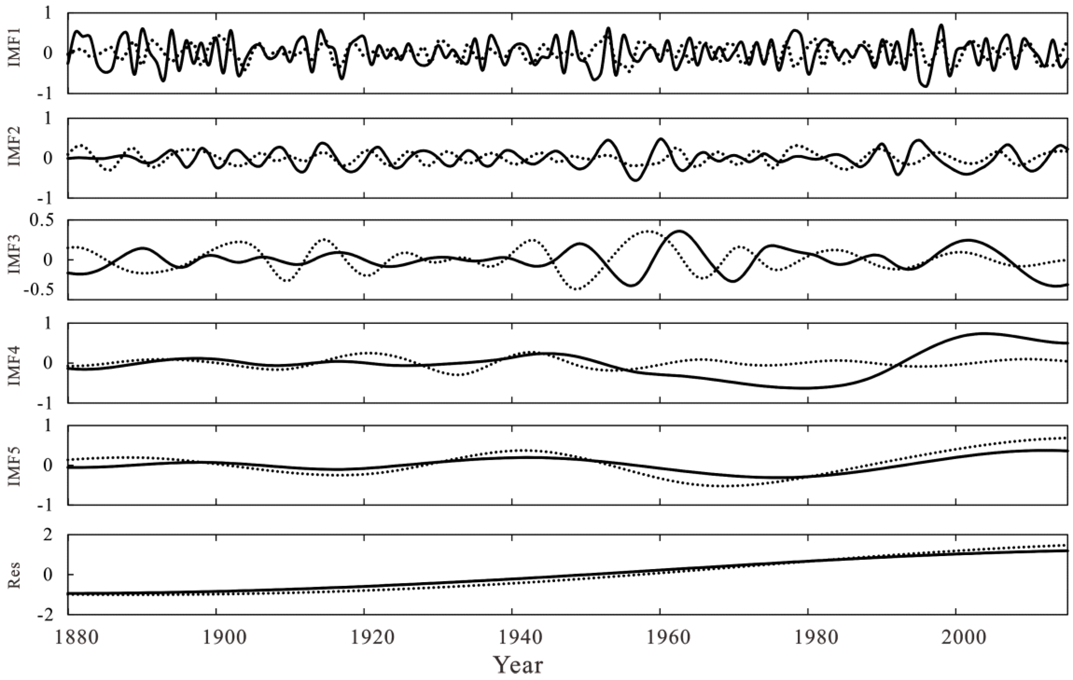
First, we used the EMD method to decompose the temperature anomaly for Shanghai and globally into five IMFs and one trend term, as shown in
Figure 4. Five IMFs indicated that, both in Shanghai and globally, there were different temperature changing rules in different time scales, while the residual term revealed that the Shanghai and global temperatures have almost the same trend.
The Fast Fourier Transform (FFT) was applied then to obtain the main cycle of each IMF component.
Table 1 lists the main cycle of each IMF component. It was obvious that the Shanghai and global temperature changes had the same cycle in the time scale of 15 years (IMF3), 23 years (IMF4), and 68 years (IMF5).
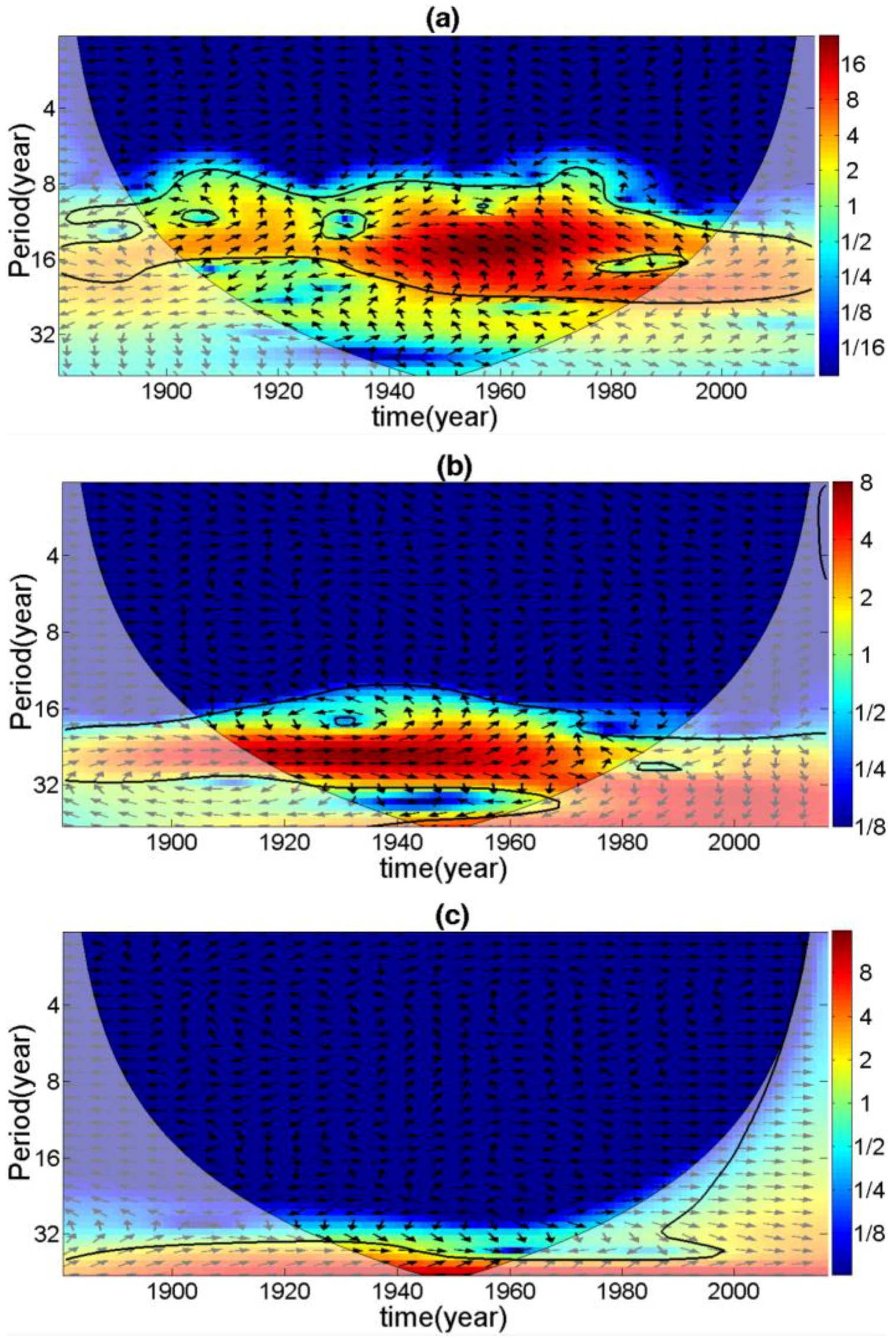
Finally, we applied a cross wavelet analysis to these three IMF components, and the results are shown in
Figure 5.
For the IMF3 component, its main cycle was about 15 years. The cross wavelet analysis showed that the temperature change phase of Shanghai was opposite to the global change phase, which means that the Shanghai temperature change lagged behind the global by about half a cycle (about 7.5 years) in the time scale of 15 years. When the global temperature rose to its highest phase, the Shanghai temperature started to rise. When the global temperature went to its lowest phase, the Shanghai temperature rose to the highest phase in its change cycle and then declined.
The IMF4 component was relatively complex, and its main cycle was about 23 years. However, after 1945, it did not show an obvious 23-year cycle. Instead, the 68-year cycle became significant. Applying the cross wavelet analysis to the main cycle (23 years) (
Figure 4b) revealed that the Shanghai and global temperatures appeared to have complex changing rules. The temperature change phase of Shanghai kept the same pace with or slightly lagged behind the global phase. However, this relationship is not stable. In addition, the CORRCOEF between this IMF component and the original time series did not pass the 95% confidence test.
The most important component was the IMF5. Its main cycle was 68 years. The CORRCOEF between this IMF and the original time series was over 0.5, which reached the 99% significant level. A cross wavelet analysis result also indicated that the change in Shanghai temperature almost kept the same pace as the global change or lagged behind the global change by about 2–10 years during the time scale of 68 years.
Based on the above analysis, the primary conclusion was that the 68-year cycle was the most significant time scale that clearly reflected the corresponding relationship between TCT in Shanghai and global warming. In addition, the response process had features of hysteresis and uncertainty, which mainly indicated that the temperature change of Shanghai lags behind the global change by about 2–10 years.
3.1.3. The Response of Shanghai TCT to Global Warming
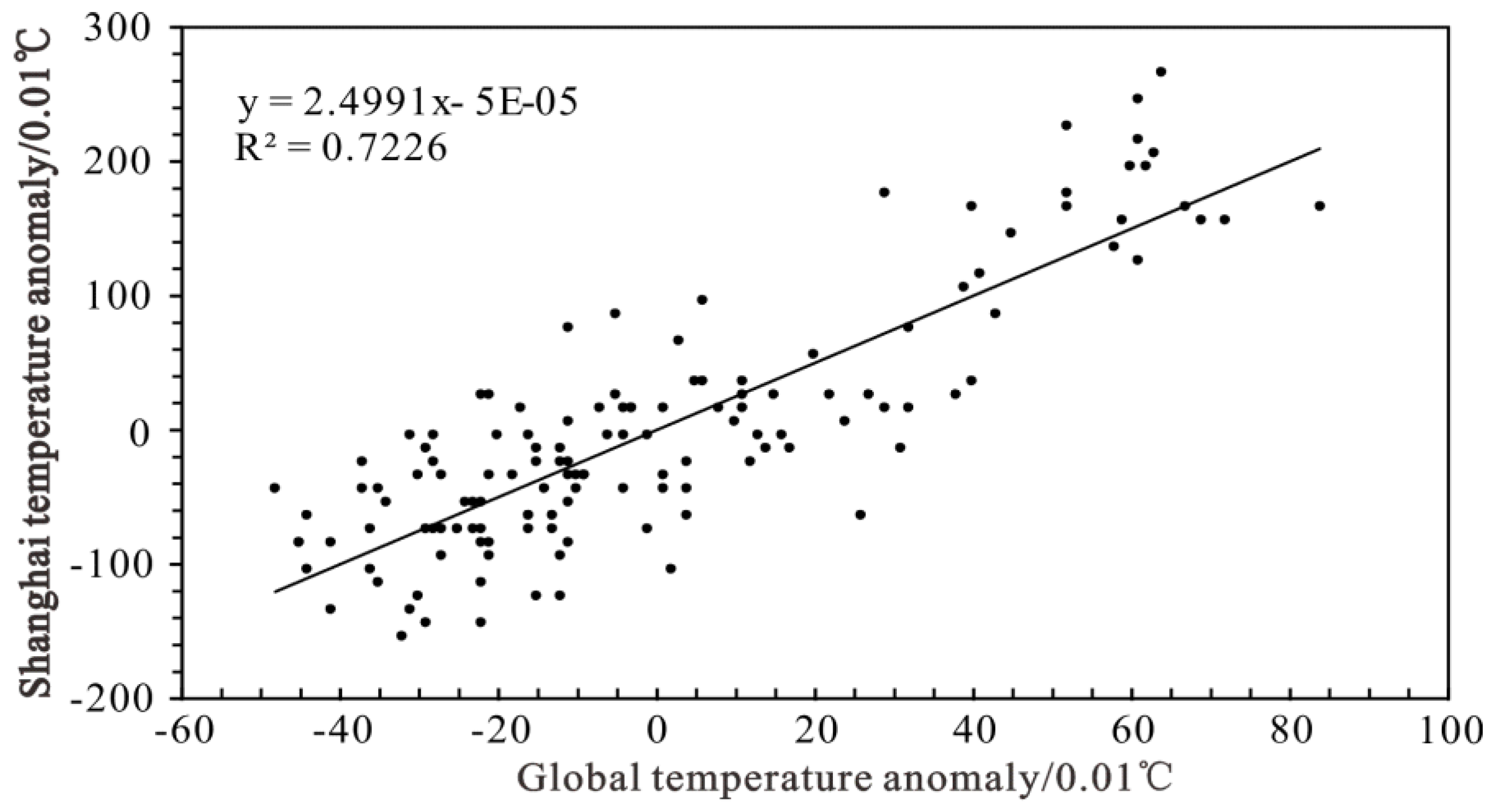
Taking the global temperature anomaly as the independent variable and the Shanghai temperature anomaly as the dependent variable, a regression equation was established.
Figure 6 shows that if the global mean temperature rose by 1 °C, the Shanghai mean temperature rose by about 2.5 °C, indicating that the Shanghai temperature change could be thought of as a strong response to global warming.
However, the Shanghai TCT was not only influenced by global warming, but its warming process could also be affected by urbanization. Therefore, we have paid attention to the effect of urbanization on the temperature change in Shanghai in the following analysis.
3.2. The Effect of Urbanization on the Temperature Change in Shanghai
In order to understand the response of temperature change in Shanghai to the urbanization process, we selected the years from 1965 to 2014, which was the typical phase of rapid urbanization in Shanghai, as our study period. We first analyzed the changing rule of the TGBXB in Shanghai and then, respectively, established the regression equations between seven socio-economic statistic indexes and the TGBXB to investigate how each index influenced the city climate. Finally, we used a principal component analysis (PCA) method to obtain a comprehensive index to reflect the urbanization level. Based on this index, we conducted further analysis on the influence of urbanization on the Shanghai temperature change.
3.2.1. The Temperature Difference between Urban and Suburban and Its Implication
TCT in Shanghai was not only influenced by urbanization but was also impacted by natural factors, such as the periodic oscillation of atmospheric circulation. Therefore, it was important to find a way to remove the impact caused by natural factors. In this study, we chose to use the temperature difference between the urban and suburban areas to remove this impact.
In the past 50 years (1965–2014), as shown in
Figure 7, the TGBXB in Shanghai increased nearly 0.4 °C, with an ARR of about 0.08 °C/10 years. This result was also found by Mu [
41]. In addition, the temperature difference would suddenly jump up 0.1 °C every 10–13 years. This result indicated that the response of the Shanghai temperature change to urbanization processes had obvious features of both continuity and rhythmicity.
3.2.2. Socio-Economic Indicators of Urbanization Affecting Temperature Change
Seven socio-economic indexes, including the city population, built-up area, GDP, total energy consumption, total civil motor vehicles, city farmland area, and urban green space were chosen to reflect comprehensively the degree of urbanization [
42,
43]. These seven socio-economic indexes have been widely used to analyze the UHI effect [
44]. The city population, built-up area, and city farmland area can reflect the urban size; total energy consumption and total civil motor vehicles can reflect the amount of energy consumption and greenhouse gases emission; GDP can reflect the size of the economy; and, finally, urban green space can reflect the extent of urban greening. We established regression equations between TGBXB and each index. The results are shown in
Table 2.
By analyzing the results of the CORRCOEFs between the socio-economic indexes and TGBXB, the factors of urbanization could be divided into three classes (positive correlation, negative correlation, and not significant correlation).
The indexes of population, energy consumption, built-up area, GDP, and total civil motor vehicles showed a positive correlation with TGBXB. These indexes could represent the size and economic development level of a city. Among them, city population and GDP were two important indexes.
City population is an important index for evaluating city size. Different population distributions lead to different energy consumptions and building densities, which influence the distribution of air temperature. Analyzing the regression equation, we found that with increasing population, the TGBXB increased quickly at first, and then the rate slowed until TGBXB reached the maximum value. Finally, the trend decreased.
The GDP reflects the economic development level, through which we could know the degree of development of a city. The regression model showed that the CORRCOEF between ln (GDP) and TGBXB is 0.78, which reached a 99% confidence level. Therefore, the GDP was highly correlated with the TGBXB. Before the 1990s, the GDP increased slowly with a narrow temperature difference. However, after the 1990s, the GDP increased quickly in Shanghai. As a response, the TGBXB rose rapidly at first and then tended to be stable.
The city farmland area showed the only negative correlation with TGBXB. In the process of urbanization, city farmland area decreased along with the expansion of the built-up area. Using the regression equation and supposing that other factors in the urbanization effect would not change, the TGBXB would rise by 0.02 °C, if 1000 hectares of farmland area were removed in Shanghai.
The final class includes urban green area, which is a unique index. Urban green space in a city is often regarded as a “green lung”. It had a strong positive correlation with urbanization level (CORRCOEF with PC1 is 0.94) but had a negative correlation with the TGBXB. The regression equation between green space area and TGBXB had a weak correlation (only –0.11). This indicated that urban green space had no obvious effect on adjustments to the climate of the entire city.
3.2.3. The Principal Component of Urbanization Effecting Temperature Change.
Table 2 shows that all the socio-economic indexes had a strong correlation with the TGBXB except for the urban green space area. The remaining six indexes could all reach the 99.9% or 99% confidence level, which indicated that they had a great influence on the TGBXB. Therefore, we can use the PCA method to extract a comprehensive index to measure the urbanization level instead of using the six indicators.
The results of the PCA method are given in
Table 3. The first principal component variance rate of these six indexes reached 97.66%, greater than 90%. Therefore, the first principal component can replace these six indicators to represent the Shanghai urbanization level.
According to the first principal component corresponding eigenvectors, the following formula can be developed
where P is the population; E is the energy consumption; S1 is the built-up area; G is the GDP; C is the numbers of civil motor vehicles; and S2 is the farmland area (all of the above data are standardized).
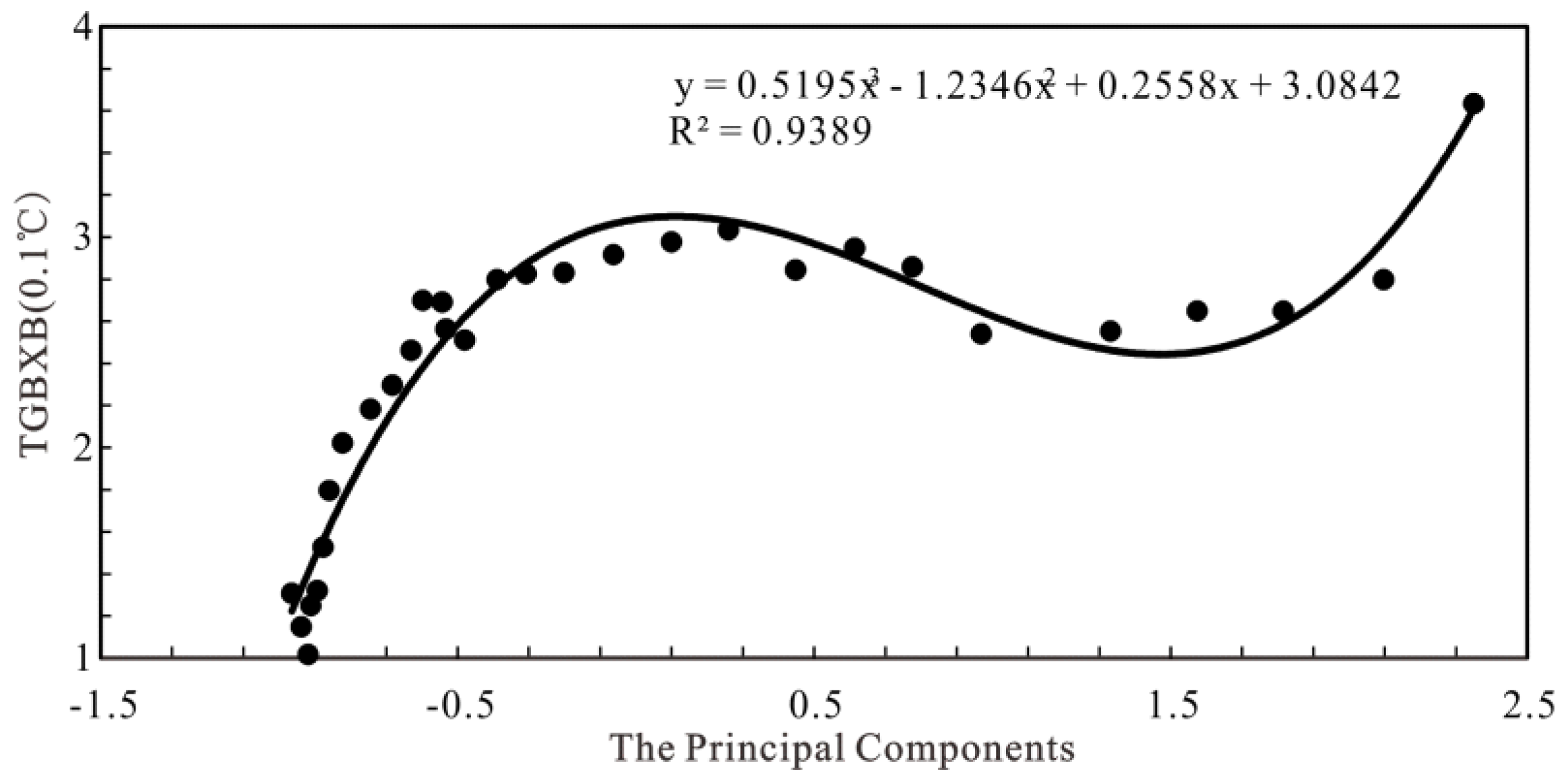
Equation (20) shows that the urbanization level was highly positive related to city population, energy consumption, built-up area, GDP, and the number of civil motor vehicles and significantly negative related to city farmland area. Therefore, the z value can be defined as the developing level of urbanization. According to the first principal component of urbanization (z value) and the smooth value of TGBXB, the relationship between them can be made into a scatter plot as shown in
Figure 8.
The TGBXB in Shanghai has a cubic relationship with the z value, and its goodness of fit is 0.94, which passed the 99.9% confidence test. The coefficient of the fitting function explained that in the low stage of urbanization (urbanization level (z value) is below 0), the TGBXB was rapidly rising with the developing urbanization. When the urbanization was in the medium stage (urbanization level (z value) between 0 and 1.5), the TGBXB showed a slowly declining trend with a deepening of the urbanization level. However, when the urbanization reached a higher stage (urbanization level (z value) is above 1.5), the TGBXB showed a significant upward trend with further urbanization.
3.3. The Frequency of Extreme Temperature Events in Shanghai
The frequency of annual extreme temperature events in Shanghai can be considered as a result of global warming and urbanization. According to the definition (
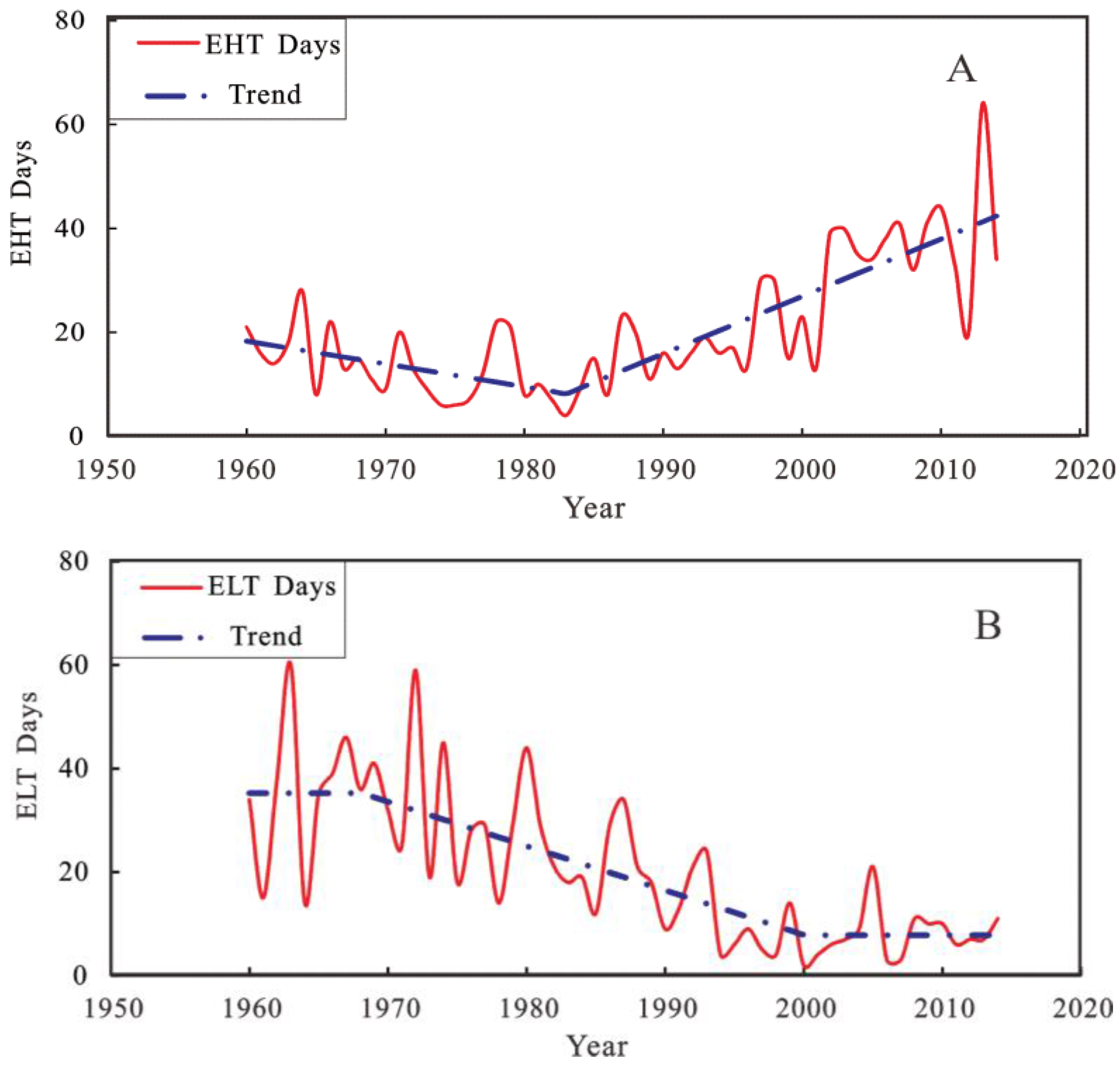
Section 2.2.7), we separately counted the annual days of EHT and ELT events in Shanghai (at the Xujiahui meteorological station) from 1960 to 2014 (
Figure 9). By using the method mentioned in
Section 2.2.6, we found that the trend of annual EHT days in Shanghai was decreasing during the years from 1960 to 1983 with a rate about −0.4 days/year. However, during the years from 1983 to 2014, the trend became significantly increasing with an ARR of about 1 day/year. As for the annual ELT days,
Figure 9B shows that the annual ELT days in Shanghai remained relatively stable with a mean value of 35.22 days/year between 1960 and 1970. However, from 1970 to 2000, the trend showed a decline with a rate of about −0.8 days/year. After 2000, the ELT days became stable again, with a mean value of 7.8 days/year established.
In order to further study the response of the Shanghai extreme temperatures to global warming and urbanization, we separately converted the annual EHT (ELT) days, GMT, and TGBXB into an annual EHT (ELT) index, GMT index, and TGBXB index, respectively, by using the normalization of the standard deviation.
Based on these indexes, we first calculated the CORRCOEF between the EHT (ELT) index and GMT index and TGBXB index, respectively. The results showed that the frequency of the annual EHT (ELT) events was highly correlated with GMT and TGBXB (rEHT-GMT = 0.67, rELT-GMT = −0.68, rEHT-TGBXB = 0.60, and rELT-TGBXB = −0.72).
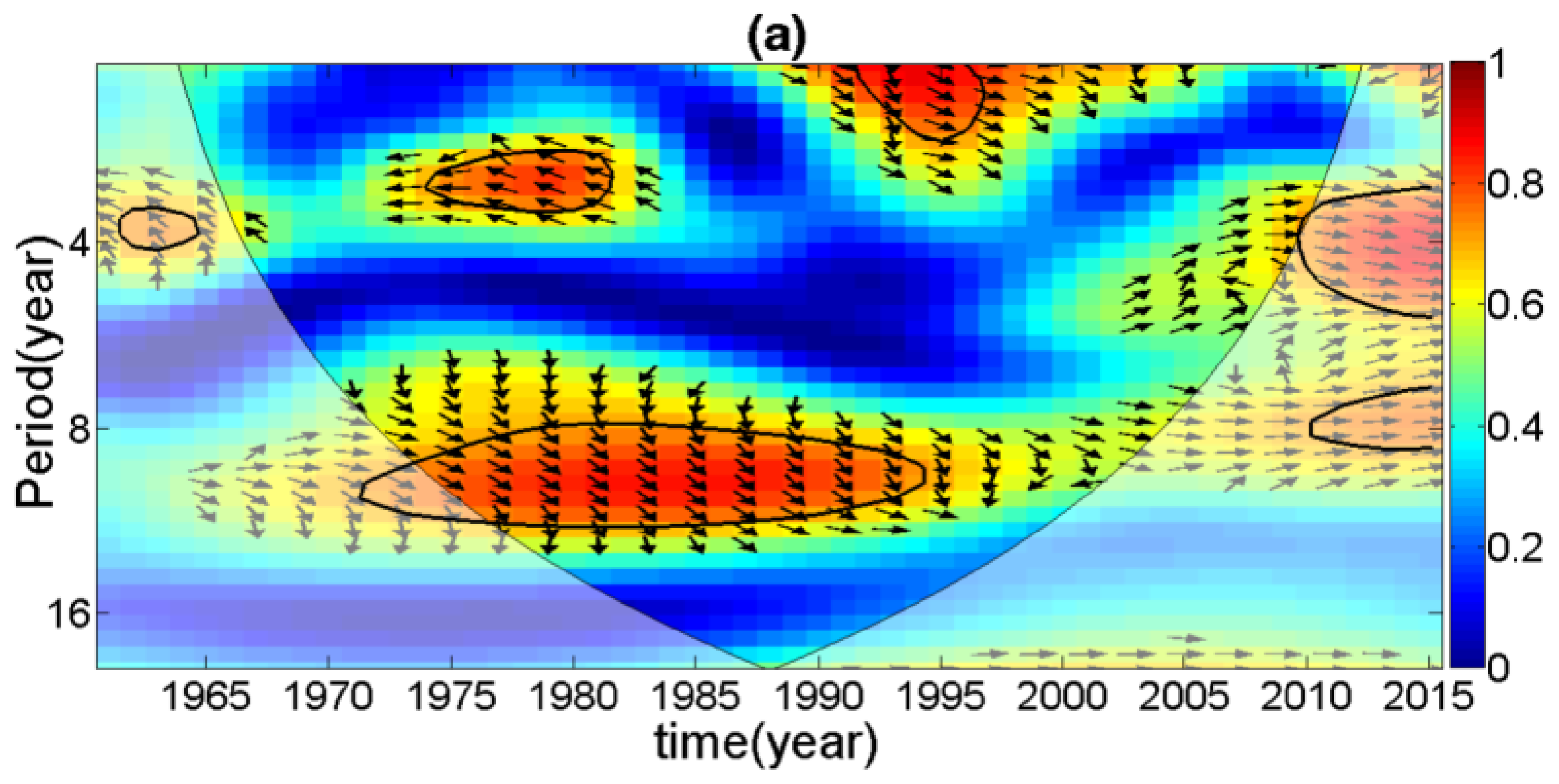
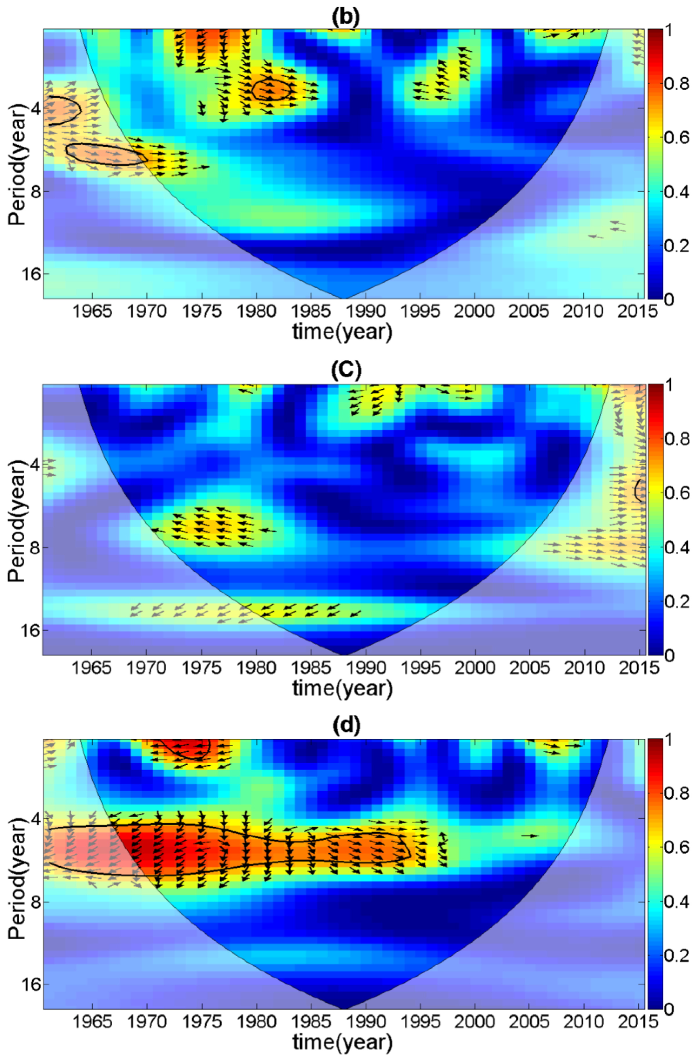
A cross wavelet analysis was used to investigate their interrelationships.
Figure 10 shows that the frequency of annual EHT events had a strong corresponding relationship with global warming, especially during the years from 1970 to 1995. The year when the GMT was on a high phase was the year when the annual EHT days were greater than average. However, the frequency of annual ELT events was not sensitive to the GMT change. Instead, the EHT events were highly correlated to the TGBXB (
Figure 10c), especially from 1960 to 1995, which indicated that urbanization was the main factor that influenced the ELT events.
4. Discussion
In
Section 3.1, we chose the M-K test instead of a t-test to determine whether the TCT of Shanghai had abrupt change points because this method did not require the data to obey a certain distribution [
22]. The results showed that the TCT for Shanghai and globally had no abrupt change points, which means that the climate change during our study period was stable; in another words, there was one climate condition. However, according to Li [
45], the Shanghai temperature had an abrupt point in 1934 based on the temperature data from 1873 to 1989. This difference may be caused by the length of the study period and the data source as different study periods will lead to different results. This is the case when we used the M-K test and temperature data from different datasets based on different statistical methods.
Concerning the EMD results, we obtained 2-year, 6-year, 15-year, 23-year, and 68-year cycles of Shanghai temperature change, which is similar to Shen [
3]. Shen [
3] and Xu [
46] suggested that the 2-year and 6-year cycles were caused by East Asian monsoons, which indicates that the East Asian monsoon can affect the short-term climate change. The 68-year cycle of Shanghai temperature change was caused by the global temperature change according to the results of this study, and the global temperature change was caused by periodical solar radiation changes according to Qian [
47]. This reveals that long-term climate change is mainly influenced by solar radiation.
In
Section 3.2, we found that GDP, population, and city farmland area were the three main factors influencing urban temperature, and the result that among all indicators of urbanization, urban population and economic development are both the important factors for the development of heat island effect in Shanghai was also confirmed by Cao [
18].
According to Gao [
48], people gather in urban areas initially and the population in suburban areas is lower, resulting in a quite significant difference in the populations between the urban and suburban areas. As urbanization increased, more and more people immigrated to Shanghai, leading to a population in the urban area close to the saturation value. Due to the supersaturation by the urban population, more and more people moved to suburban or even rural areas, leading to a more balanced population distribution. This is why the TGBXB increased at first and finally decreased with increasing population.
As for the influence of city farmland area on urban climate, Dong [
49], Pei [
50], and Gouma [
51] have also found that temperature difference increases with decreasing farmland area. In addition, Dong [
49] explained this phenomenon from the standpoint of the heat exchange between the atmosphere and land surface. In his theory, if the land type is farmland, the land surface albedo will decrease. The plants in the farmland will contain more heat, and the heat transmission from the land surface to the atmosphere will be retarded, leading to a slower temperature rise than in non-farmland areas.
We should be most concerned about the urban green areas. Although it had no obvious effect on the entire city climate in this study, according to Ge [
52], as the urban green space expands, it can increasingly affect the city climate. The z value of Shanghai was above 2 in 2015 according to the data from Shanghai statistical yearbook, which indicates that the urbanization level of Shanghai was at a relative high stage as discussed in
Section 3.2.3. At this stage, the TGBXB will rise rapidly with urbanization, so we should expand the urban green area to reduce the rising rate of the TGBXB.
Using the PCA method to extract an index to reflect the urbanization level of a city and connect it to city warming is a relative new idea. Wang and Shen [
43] have applied this idea to analyze the connection between UHI and the urbanization level. They explained the UHI change rule in the low and middle stages of urbanization. In our study, by using more socio-economic indicators and a more detailed dataset, we revealed the TGBXB change rule not only in low and middle stages, but also at higher stages of urbanization. Compared with traditional methods, such as a single index analysis, this method can quantitatively determine the level of urbanization and indicate the sensitivity of the temperature difference between urban and suburban areas to urbanization.
Section 3.3 has mainly revealed the changing trend of the frequency of the annual EHT or ELT events in Shanghai. Daniel [
13] suggested that urbanization can strongly affect minimum temperature, and Deng [
53] suggested that global warming has increased the frequency of EHT events in the Yangtze River delta during the past 120 years. With these views and our data, a solid conclusion can be made that the frequency of annual EHT events was mainly controlled by global warming, while the frequency of the annual ELT events was mainly impacted by urbanization.
However, we still have questions remaining for further studies. As mentioned, the IMF4 component cannot pass the 95% confidence test. Before 1945, it showed an obvious 23-year cycle; but after 1945, a 68-year cycle became significant. We considered it a random fluctuation between a meso-scale cycle (15 years) and a long cycle (68 years). The physical mechanism that caused this fluctuation remains unknown. The second question surrounds the prediction of climate change based on these results. A neural network algorithm was proposed by Rumelhart and McCelland [
54] in 1986. It is now widely used to predict hydrological and meteorological processes. Based on the EMD results, we can use a BP neural network algorithm to simulate climate change in future studies. Besides, it was a pity that we cannot use the same data length in
Section 3.2 and
Section 3.3 because Shanghai social-economic data before 1965 are not available to the public.
5. Conclusions
The main objective of this paper is to find out the response of TCT in Shanghai to global warming and urbanization. Through the above analysis, we can draw the following conclusions:
(1) TCT of Shanghai displayed 2-year, 6-year, 15-year, 23-year and 68-year periodic fluctuation, which was similar to global in the past 135 years. However, warming strength in Shanghai was stronger than global warming. The corresponding relationship between Shanghai and global temperature was obvious and had the features of similarity and hysteresis in the middle-long cycles. Similarities include that both Shanghai and global annual mean temperature have obvious cycle of 15 years and 68 years with a 23 years long-term fluctuation. Hysteresis refers to the fact that Shanghai temperature change lags behind global change.
(2) In recent decades, rapid urbanization process has significantly pushed up the annual mean temperature of Shanghai and widened the TGBXB with the features of continuity, stage and rhythmic. TGBXB in Shanghai had unique increasing trend, showing that TGBXB would suddenly jump 0.1 °C every 10 to 13 years (ARR is 0.08 °C/10 years). The various indicators in the urbanization had different influence on TGBXB. Among these indicators, the increasing of population and GDP and the decreasing of city farmland were three main factors that lead to strong UHI event. Urban green space could regulate the microclimate [
53], but it had only a small impact on the whole city climate.
(3) In different levels of urbanization, the contribution of urbanization to urban warming is different, which is specific performance in that with the deepening of urbanization, TGBXB rises rapidly at first, then it turns to a decreasing trend, and finally returns to a significant upward trend.
(4) The frequency of annual EHT events has strong correlation with global warming, whereas the frequency of annual ELT events is sensitive to urbanization process. With global warming strengthening [
5] and urbanization process continuing, the frequency of annual EHT events will become higher, while the frequency of annual ELT events will become lower in the future.


