An Improved Iterative Fitting Method to Estimate Nocturnal Residual Layer Height

Abstract

The planetary boundary layer (PBL) is an atmospheric region near the Earth’s surface. It is significant for weather forecasting and for the study of air quality and climate. In this study, the top of nocturnal residual layers—which are what remain of the daytime mixing layer—are estimated by an elastic backscatter Lidar in Wuhan (30.5°N, 114.4°E), a city in Central China. The ideal profile fitting method is widely applied to determine the nocturnal residual layer height (RLH) from Lidar data. However, the method is seriously affected by an optical thick layer. Thus, we propose an improved iterative fitting method to eliminate the optical thick layer effect on RLH detection using Lidar. Two typical case studies observed by elastic Lidar are presented to demonstrate the theory and advantage of the proposed method. Results of case analysis indicate that the improved method is more practical and precise than profile-fitting, gradient, and wavelet covariance transform method in terms of nocturnal RLH evaluation under low cloud conditions. Long-term observations of RLH performed with ideal profile fitting and improved methods were carried out in Wuhan from 28 May 2011 to 17 June 2016. Comparisons of Lidar-derived RLHs with the two types of methods verify that the improved solution is practical. Statistical analysis of a six-year Lidar signal was conducted to reveal the monthly average values of nocturnal RLH in Wuhan. A clear RLH monthly cycle with a maximum mean height of about 1.8 km above ground level was observed in August, and a minimum height of about 0.7 km was observed in January. The variation in monthly mean RLH displays an obvious quarterly dependence, which coincides with the annual variation in local surface temperature.

1. Introduction

The planetary boundary layer (PBL) is an atmospheric region near the Earth’s surface affected by surface frictional resistance [1,2,3]. The entrainment layer at the top of the boundary layer exerts a partial blocking effect on the dispersion of surface pollutants; this effect results in a high concentration of near-surface contaminants [4,5,6]. Therefore, accurate determination of PBL height is significant for weather forecasting and studying air quality and climate [7,8]. The convectively-driven PBL is known as a convective boundary layer (CBL) that develops about half an hour after sunrise, and nocturnal residual layers (RL) are what remain of the daytime CBL [1]. Studying the urban nocturnal RL height (RLH) is important for the accurate modelling of air quality [9].

Continuous elastic Lidar measurement with high spatial and temporal resolution allows for the estimation of the diurnal cycle of RLH [4,10,11]. Three Lidar methods used to obtain RLH are the ideal profile-fitting (IPF) [12], gradient (Grad) [5,8,13], and wavelet covariance transform (WCT) methods [10,14,15]. The IPF method is utilized to obtain RLH by fitting the Lidar signal or particle backscatter coefficient to an idealized profile [12]. The Grad method determines RLH as the gradient maximum of the Lidar signal profile [5,8,13]. The WCT method analyzes the vertical gradients of aerosol and the fast temporal changes in the signal time series as a function of height, and is less affected by signal noise compared to gradient methods [10,14,15]. The work of Summa et al. [16] demonstrates a dependency of PBL height on temperature, which can be applied to estimate diurnal CBL height and nocturnal RLH from the identification of minima in the first-order derivative of the logarithm of the range-corrected rotational Raman Lidar signals. However, RLH determination with Lidar is affected by strong backscatter layers, such as clouds and optical thick aerosols (e.g., mineral dust aerosol) [14,17,18]. These layers cause strong peaks in the range-corrected Lidar signal, and these peaks may cause large errors in RLH detection. Therefore, we propose an improved iterative fitting method based on the IPF method to eliminate the optical thick layer effect on RLH detection using Lidar signals. The improved method can find the optical thick layer and remove it gradually.

In this study, two typical cases are used to demonstrate the theory and advantage of the proposed method. Then, six-year measurements (from 28 May 2011 to 17 June 2016) are conducted to compare the simultaneous RLHs evaluated by IPF and the proposed improved method. The frequency distribution of long-term RLHs derived from the improved method is also revealed. Lastly, IPF and the proposed improved method based on elastic Lidar backscatter signals are used to evaluate long-term monthly RLHs.

2. Experimental Methods

The elastic Lidar system operates at the top of a building in the State Key Laboratory of Information Engineering in Surveying, Mapping, and Remote Sensing (30°32′N, 114°21′E and 28 m above sea level) at Wuhan University, Wuhan City, Hubei Province, China [19,20]. The backscatter signals of the elastic Lidar are recorded every minute. The vertical range resolution of the elastic Lidar profile is 7.5 m. Twenty-minute averaged Lidar signals—which can improve the signal-to-noise ratio—are applied in this study.

Aerosol vertical distribution is strongly influenced by PBL thermal structures. The concentration of pollutants on the mixing layer is higher than that on the upper layer, which leads to a sharp gradient in the Lidar signal profiles near the top of the PBL. The characteristic of PBL is associated with CBL height at daytime and with RLH during nighttime [21]. The IPF method is widely applied in Lidar observations to determine RLH [10,22].

2.1. IFP Method

Steyn (1999) proposed the IPF method, which obtains the PBL parameters by fitting a Lidar-derived backscatter profile to an idealized backscatter profile B(r). The idealized backscatter profile B(r) can be expressed as [10,12]

$$B(r)=\frac{B_m+B_{\mu }}{2}-\frac{B_m-B_{\mu }}{2}erf\left(\frac{r-r_m}{s}\right)$$

(1)

where B_m is the mean mixed layer backscatter, B_u is the mean backscatter in the air immediately above the mixed layer, r_m is the mixed layer depth, and s is related to the thickness of the entrainment layer. The least square fitting method is applied to minimize the root-mean-square deviation between the idealized backscatter profile B(z) and the Lidar-derived backscatter profile. Thereafter, the four idealized backscatter profile parameters in Equation (1) can be determined. The thickness of the entrainment zone is equal to 2.77s, where s is the thickness of the layer in which layer air and overlying air are mixed.

The range-corrected signal (RCS) of Lidar is applied to estimate RLH in this study. The Lidar RCS is defined as

$$X(r)=[P(r)-b]r^2$$

(2)

where P(r) refers to the elastic Lidar equation [23,24]

$$P(r)=\frac{C[{\beta }_p(r)+{\beta }_m(r)]\cdot T^2(r)}{r^2}+b$$

(3)

where P(r) is the Lidar signal at an altitude of r; C includes all system independent parameters, such as Lidar system constant and transmitting energy; β_p and β_m represent particle and molecule backscattering coefficients, respectively; T(r) refers to the single-way atmospheric transmission; and b represents background noise.

The RLH detection algorithm searches for strong decrements in the Lidar signal with height. However, clouds are characterized by a steep increase in RCS at the cloud base, followed by a strong decrease in the signal with increasing cloud penetration depth. Thus, RLH determination with Lidar-measured RCS is affected by cloud layers with strong backscatter signals [14,17,18]. To eliminate the cloud layer effects, we propose an improved iterative fitting method to determine RLH.

2.2. Improved Method

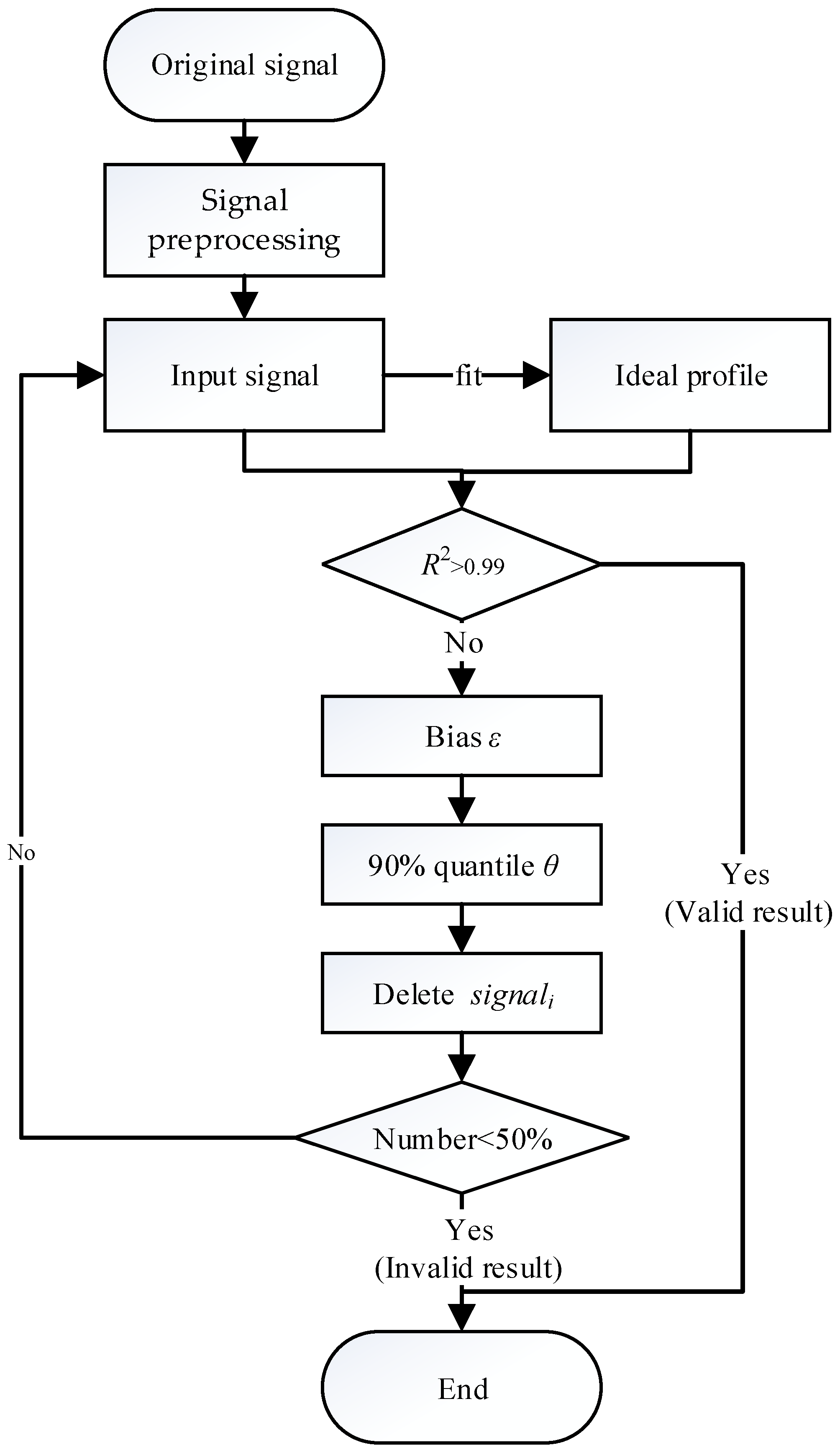
The improved iterative fitting method requires the IPF method to accurately obtain the region where aerosols decrease dramatically in the first iteration. However, the IPF method may regard the cloud base as RLH when the cloud layer is thick, which can be seen in the second case analysis. Therefore, signal preprocessing is necessary. To avoid misjudgment of the IPF method in the first iteration, the backscatter signals where intensity is larger than the surface signal intensity (below 0.3 km) are removed first.

After signal preprocessing, an idealized fitting profile can be obtained by fitting the Lidar-derived backscatter profile with the IPF method. Cloud layer is characterized by a strong backscatter signal. Thus, the Lidar-derived backscatter signal at a given altitude with a cloud layer is larger than the idealized fitting profile value at the corresponding height. To identify the Lidar-derived signal with an optical thick layer, the bias (ε) between the Lidar-derived signal and the idealized ideal profile is calculated. The Lidar-derived signal at the altitude where bias (ε) is larger than the threshold value is regarded as an optical thick layer. The threshold value is defined as 90% quantile (θ) of the bias (ε), which is determined through several experiments. After deleting the Lidar-derived signal with an optical thick layer for the first time, we obtained the improved Lidar-derived signal profile. By reapplying the IPF method, now to the improved Lidar-derived signal, we obtain an improved idealized fitting profile. To remove the optical thick layer further, the bias (ε) between the improved Lidar-derived signal and the improved idealized fitting profile needs to be calculated. After removing the Lidar-derived signal with a cloud layer, we further improve the signal profile. Multiple iterations are conducted until the fitting decision coefficient (R²) is greater than 0.99 to remove the cloud layer. However, if the number of improved signals is less than 50% of the number of original signals before the fitting decision coefficient reaches 0.99, the iteration stops with an invalid result. The flowchart of the improved iterative fitting method is shown in Figure 1. The main iterative steps are as follows:

(1)

Signal preprocessing. The backscatter signals where intensity is larger than the surface signal intensity (below 0.3 km) are removed.

(2)

Fit input signal by IPF method to obtain an ideal profile. Input signal refers to the preprocessed Lidar-derived backscatter signal in the first iteration. Then, the improved signal serves as the input signal in later iteration.

(3)

Calculate the fitting decision coefficient R² between the input signal and the ideal profile. If R² is greater than 0.99, the iteration stops with a valid result. If not, continue iteration.

(4)

Calculate bias ε between the input signal and the ideal profile.

(5)

Calculate 90% quantile θ of the bias ε, which is a threshold value to judge optical thick layer.

(6)

Delete the signal_i (subscript i refers to the altitude at each point) where ε_i is greater than θ, because the signal_i at the altitude where ε_i is greater than θ is regarded as optical thick layer.

(7)

Calculate the number of the improved signal. If the number of the improved signal is less than 50% of the number of original signal, the iteration stops with an unusable result. If not, continue iteration.

(8)

Fit the improved signal by reapplying the IPF method to obtain an improved ideal profile.

Repeat steps (2)–(8) until the number of improved signal is less than 50% of the number of the original signal (invalid result) or until the fitting decision coefficient R² is greater than 0.99 (valid result).

3. Case Analysis

Two cases—which represent the typical evolution of nocturnal RLHs from Lidar-measured RCSs with thin and thick clouds—were analyzed. The theory and performance of the improved iterative fitting method is also demonstrated in this section.

3.1. Case Study 1 (29 November 2013)

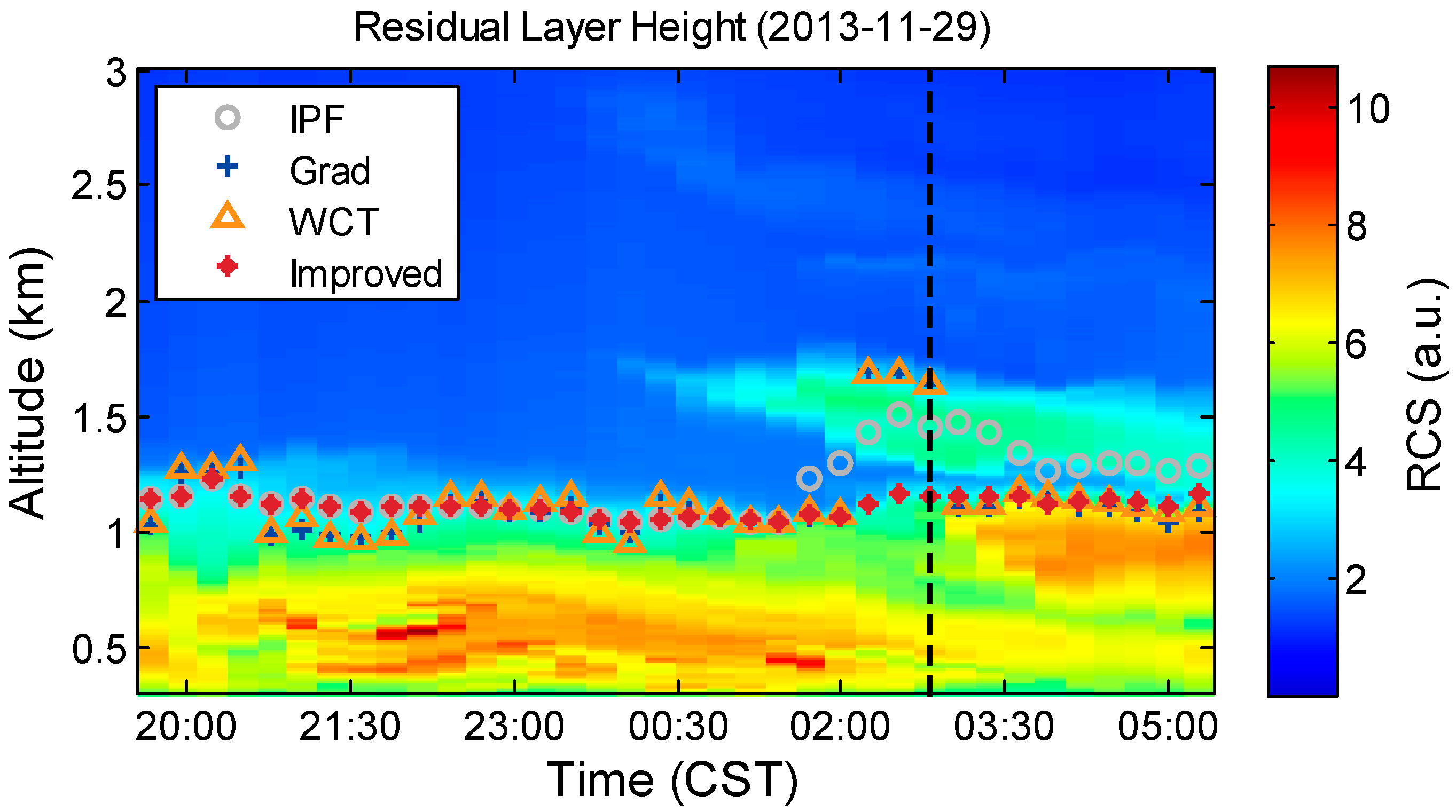
Figure 2 shows Lidar-measured RCS data (20 min/7.5 m resolution) and the RLHs estimated with IPF, Grad, WCT, and improved methods throughout an entire night. The evolution of RLH is visible from the time–height contour of RCS (Figure 2). The results derived from IPF, Grad, WCT, and the improved method coincide before 2:00 on 30 November 2013 Chinese Standard Time (CST) under cloudless conditions. Thin cloud layers are clearly visible at 1.2–1.8 km after 2:00. Aerosols mainly exist below 1 km, as shown in Figure 2. The RLHs estimated with IPF, gradient, and WCT methods are clearly affected by the thin cloud layer above RL. The obviously inaccurate results of the IPF and Grad methods at 02:00–03:00 are attributed to the high cloud tops regarded as RLHs. The cloud layer also lends to an overestimation of RLH derived from the IPF method. The reason is explained in the next paragraph, which presents a single RCS profile analysis. Good agreement exists among IPF, Grad, WCT, and improved methods when the cloud layer is thin or nonexistent. The practicality of the improved method is demonstrated in this case analysis, especially under the effects of a low cloud layer.

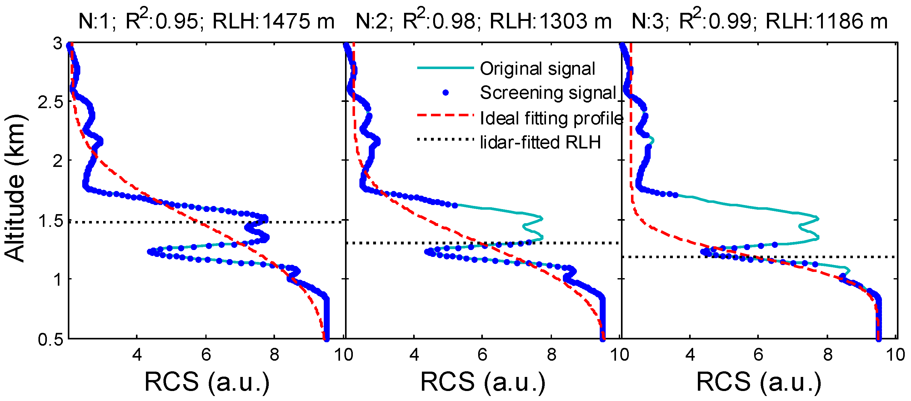
Figure 3 presents a case that involves a cloud layer near the top of the RL, which corresponds to the black dotted line in Figure 2. When iteration number N is equal to 1, the cloud layers exert a significant influence on RLH detection. The IPF method provides an unreasonable RLH in the cloud layer, with a low determination coefficient (R² = 0.95). The cloud layers at 1.2–1.8 km (which seriously affect the fitting results) can be removed gradually by the improved method. After three iterations (i.e., N = 3), an authentic result (1186 m) with perfect fitting (R² = 0.99) is obtained.

3.2. Case Study 2 (12 May 2015)

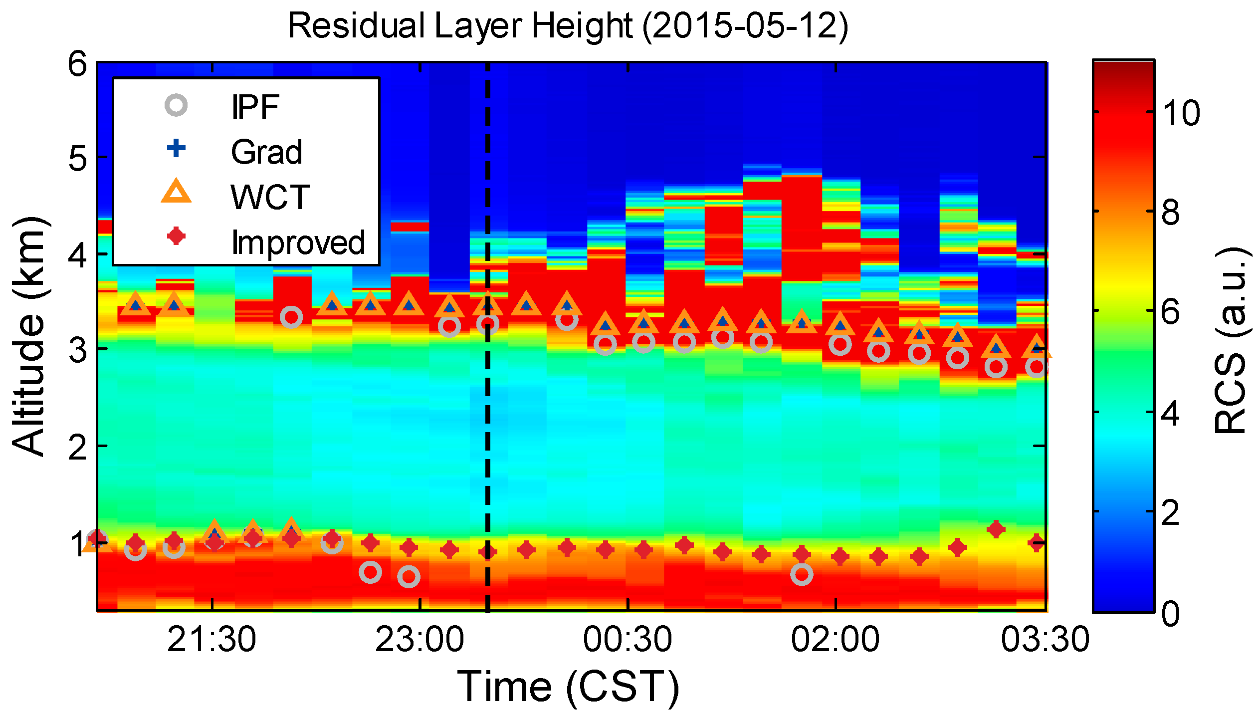
Figure 4 shows the time–height contour plots (20 min/7.5 m resolution) of the Lidar-measured RCS and RLHs estimated with the IPF, gradient, WCT, and improved methods. The evolution of RLH (the top of the aerosol layer) is visually manifested by the color contour plots of RCS. Based on the RCS shown in Figure 4, the RLHs are calculated with the various methods. As shown in Figure 4, the RLs exhibit minimal variation between 20:00 and 03:30 CST on the following day. The height reaches ~1.0 km. However, IPF, gradient, and WCT methods overestimate the RLHs (~3.0 km), especially after 23:00. The thick cloudy layers at 3–4 km contribute to the misjudgment of the three methods. The improved method shows a good performance in RLH detection in this case. The thick cloudy layers exert a small effect on the improved method. To explain the misjudgment of the IPF method and to show the functionality of the improved method, we select a RCS profile at 23:28, 12 May 2015 (CST), which corresponds to the black dotted line in Figure 4.

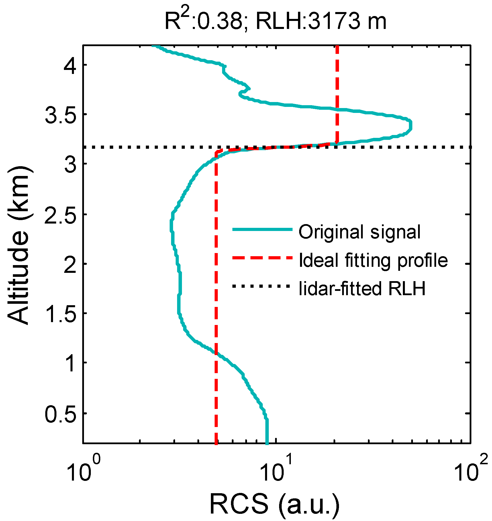
Figure 5 presents the 20-min averaged profile of RCS and the corresponding ideal fitting profile from the IPF method. The black dotted line in Figure 5 refers to the IPF-derived RLH. The IPF method regards the cloud base as RLH and provides an overestimated RLH (3173 m). A low determination coefficient (R² = 0.38) indicates that the fitting result is poor. The backscatter signal intensity of the cloud layer at 3–4 km is about one order of magnitude larger than the surface signal intensity (below 0.5 km), which causes the IPF method to fail to accurately obtain the region where aerosols decrease dramatically.

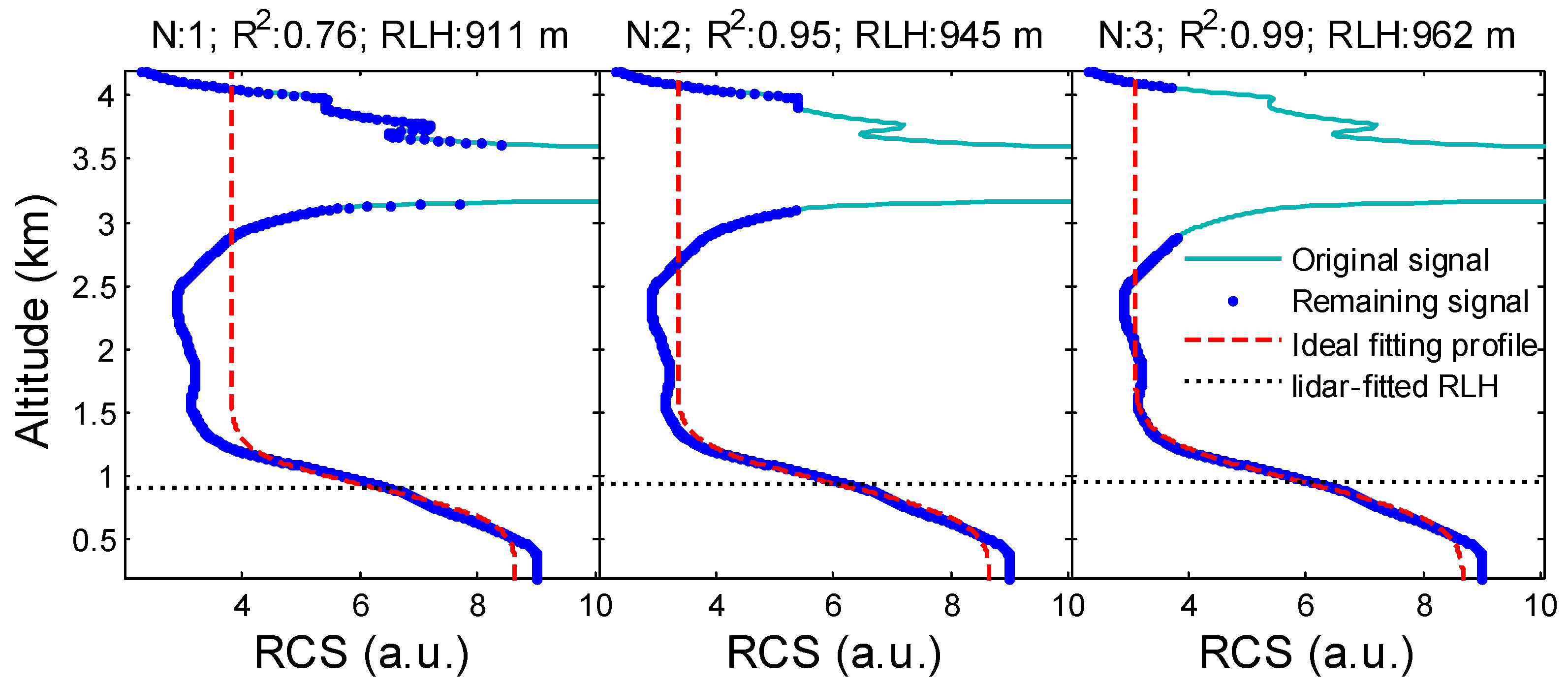
The 20-min mean RCS profile and the corresponding ideal fitting profile from the improved method (Figure 6) display the theory of the improved method for RLH evolution. To avoid misjudgment in the improved method before the first iteration, the backscatter signals where intensity is larger than the surface signal intensity (below 0.3 km) are removed first. This is signal preprocessing as shown in Figure 1. Second, the improved method can be applied to evaluate RLH. Figure 6 shows that the improved method can accurately identify the region where aerosols decrease dramatically, despite the cloud layer exerting a significant influence on RLH detection in the first iteration. The IPF method provides an RLH with a low determination coefficient (R² = 0.76), which indicates that the accuracy of the RLH is poor. Large deviations between the original signal and the ideal fitting profile can also be found at 1.5–3.0 km. After three iterations (i.e., N = 3), an expected authentic result (962 m) with perfect fitting (R² = 0.99) is obtained. The thick cloud layers at 3.0–4.0 km—which seriously affect the fitting results—can be removed gradually.

4. Long-Term Analysis

Statistical analysis data were measured by elastic Lidar at no-rain nighttime (i.e., 20:00–05:00 CST) from 28 May 2011 to 17 June 2016. The temporal resolution of the retrieved results was 20 min, and 357 days were available at all times. A large amount of data was missing during the measured period. The reason is that our elastic Lidar is a self-developing Lidar with many measurements used only for signal tuning. Moreover, many observation times were overlooked because of maintenance of the elastic Lidar system. Furthermore, we only analyzed the signal with obvious nocturnal RLH. Our elastic Lidar cannot measure under rainy or other severe weather conditions. The valid case in the long-term analysis is 6137. The invalid value from the improved method was discarded in the following analysis. Therefore, the statistical results may not completely represent the true results because of inadequate measurement data.

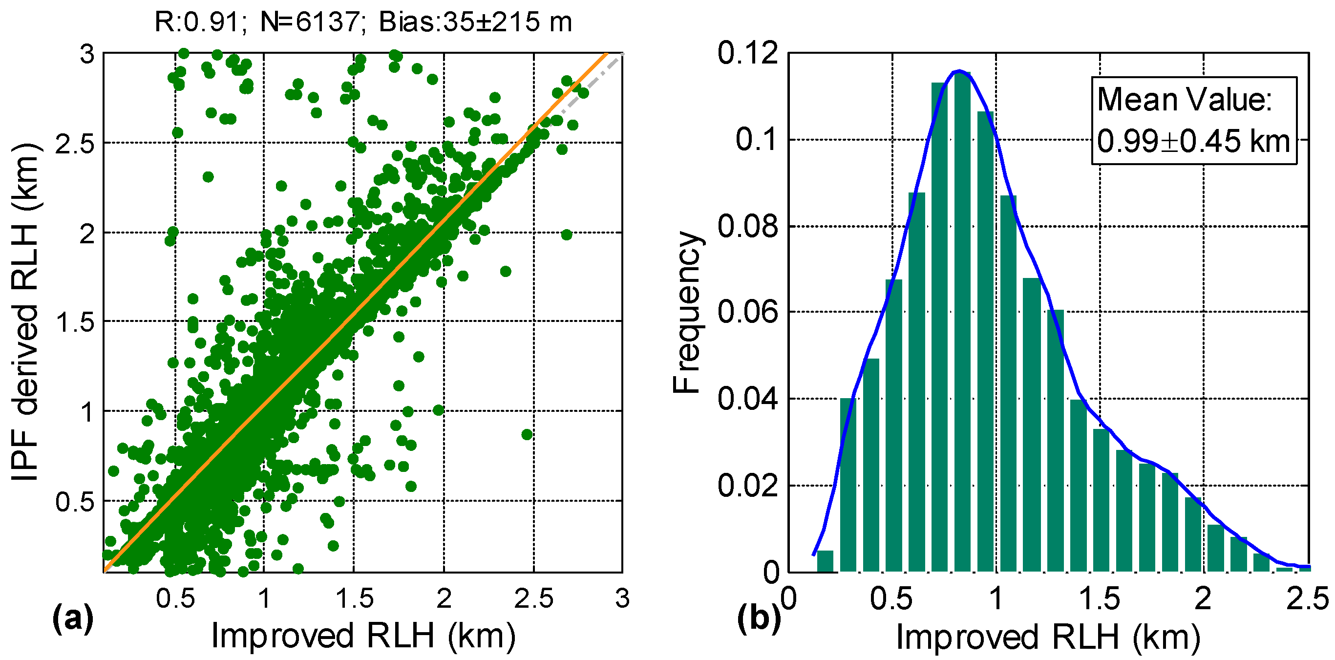
The improved iterative fitting approach described above is tested in long-term studies to evaluate its applicability. Figure 7a compares the 20-min average RLHs obtained with the improved method to the 20-min mean RLHs estimated by the IPF method from Lidar-derived RCS. The statistical parameters (correlation coefficient R, number of comparisons N, and bias) for the study are plotted on top of each subfigure. N, which is the valid number for comparison, is defined as the range of RLH from 0.2–3 km to avoid the effects of incomplete overlap correction below 0.2 km. The correlation coefficients (R) for Figure 7a are 0.91, and the bias is 35 ± 215 m. The high correlation coefficient and low bias reveal the consistency of RLHs obtained from the improved and IPF methods. However, several IPF-derived RLHs are higher than the corresponding improved RLHs, which may contribute to the influence of the low cloud layer.

The practicablity of the improved method is proven by the two case analyses and the correlation analysis between the improved and IPF methods. Therefore, we only used the improved RLHs to demonstrate the frequency distribution of RLHs. Figure 7b presents the frequency distribution of RLHs derived with the improved method during measurement periods. Most of the RLHs range from 0.5–1.3 km, with a peak value of 0.8 km and a mean value of 0.99 ± 0.45 km.

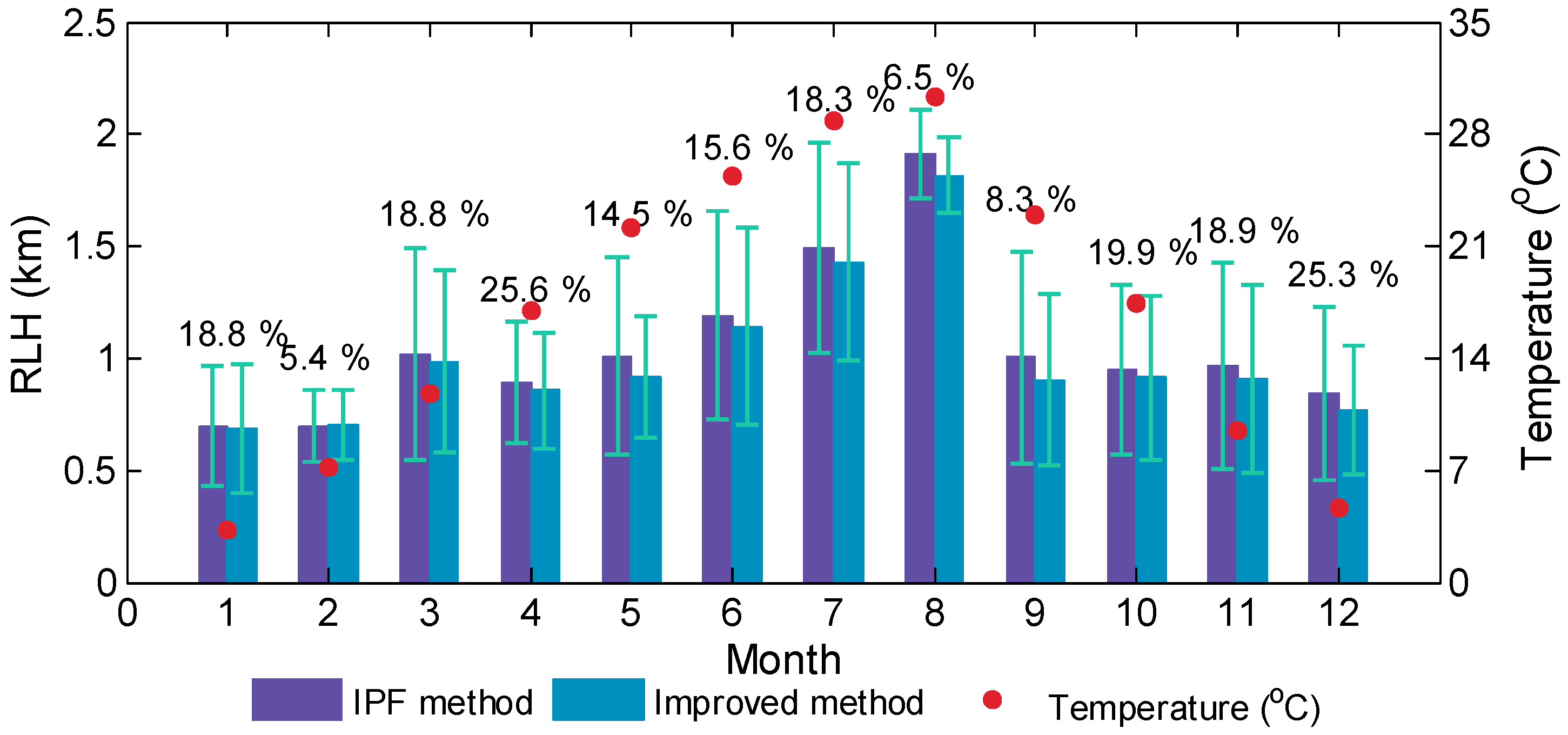
Figure 8 shows the monthly mean RLHs derived with IPF and the improved methods with Lidar measurements in Wuhan during the entire study period. The red circles refer to the mean temperature (°C) based on the same measuring days of the Lidar for each month. The percentage of available days in each month during the six years are plotted in the same figure. For all months, the RLHs derived by the improved method are less than those derived by the IPF method. This finding may indicate that some overestimations occur in the results of the IPF method. The two case analyses determine the overestimates when low cloud layers appear. The decrease in standard deviations (i.e., the error bar in Figure 8) of the improved method indicates that the variation ranges of IPF-obtained RLH are also overestimated.

The monthly variation in RLH is also obtained based on the statistical analysis of monthly survey data. A clear RLH monthly cycle is also found through monthly survey data statistical analysis, with the maximum mean height reaching approximately 1.8 km above ground level in August and the minimum height reaching approximately 0.7 km in January. The monthly mean values of temperatures are also plotted as red dots in Figure 8. In summer over Wuhan, the atmosphere’s convective motions become frequent and intense because of the strong solar radiation and high surface temperature, which cause the diffusion of aerosol particles and pollutants. Therefore, the RLHs during this time are higher than those during the cold months. In summer (winter), strong (weak) atmospheric convective motions under high (low) temperatures result in high (low) RLH. Similar conclusions about the relationship between RLH and temperature have been reported in several previous studies [25,26]. The variation in the monthly mean RLH displays an obvious quarterly dependence, which coincides with the annual variation in the local surface temperature. However, an accurate evaluation of the relationship may require additional continued observations.

5. Conclusions

Long-term RLHs are evaluated and studied by IPF and the improved method with elastic Lidar RCS measured from 28 May 2011 to 17 June 2016 at Wuhan University. The improved iterative fitting method is proposed to eliminate the optical thick layer effect on RLH detection. Two typical case analyses are performed to evaluate the performance of the proposed improved method. The analyses reveal that the improved method is more practical and precise for nocturnal RLH evaluation than IPF, Grad, and WCT methods under low cloud conditions. The comparison of long-term 20-min average RLHs obtained with the improved and IPF methods from Lidar-derived RCS shows a high correlation coefficient and low bias, which indicate the consistency of RLHs obtained with the two methods. However, several IPF-derived RLHs are higher than the corresponding improved RLHs, which may contribute to the influence of the low cloud layer. The frequency distribution of RLHs derived with the improved method shows that most of the RLHs range from 0.5–1.3 km, with a peak value of 0.8 km and a mean value of 0.99 ± 0.45 km. On the basis of a statistical analysis of six-year Lidar data, the monthly mean Lidar-derived RLHs from IPF and the improved method around the Lidar site in Wuhan are reported. A clear RLH monthly cycle is found, with the maximum mean height of about 1.8 km above ground level in August and the minimum height of about 0.7 km in January. The variation in the monthly mean RLH displays an obvious quarterly dependence, which coincides with the annual variation in the local surface temperature.

Future studies should determine the nocturnal RLH using multiple tools and methods. The relationships between RLH and other optical parameters or synoptic conditions require in-depth study. Moreover, the improved method can also be applied in the evaluation of PBL height at daytime.

References

- Stull, R.B. An Introduction to Boundary Layer Meteorology; Kluwer Academic Publishers: Dordrecht, The Netherlands, 1988. [Google Scholar]
- Zhang, Y.; Gao, Z.; Li, D.; Li, Y.; Zhang, N.; Zhao, X.; Chen, J. On the computation of planetary boundary-layer height using the bulk richardson number method. Geos. Model Dev. 2014, 7, 2599–2611. [Google Scholar] [CrossRef]
- Zhang, Y.; Seidel, D.J.; Zhang, S. Trends in planetary boundary layer height over Europe. J. Clim. 2013, 26, 10071–10076. [Google Scholar] [CrossRef]
- Granados-Muñoz, M.; Navas-Guzmán, F.; Bravo-Aranda, J.; Guerrero-Rascado, J.; Lyamani, H.; Fernández-Gálvez, J.; Alados-Arboledas, L. Automatic determination of the planetary boundary layer height using Lidar: One-year analysis over southeastern spain. J. Geophys. Res. 2012. [Google Scholar] [CrossRef]
- Luo, T.; Yuan, R.; Wang, Z. Lidar-based remote sensing of atmospheric boundary layer height over land and ocean. Atmos. Meas. Tech. 2014, 7, 173–182. [Google Scholar] [CrossRef]
- Bravo-Aranda, J.A.; Titos, G.; Granados-Muñoz, M.J.; Guerrero-Rascado, J.L.; Navas-Guzmán, F.; Valenzuela, A.; Lyamani, H.; Olmo, F.J.; Andrey, J.; Alados-Arboledas, L. Study of mineral dust entrainment in the planetary boundary layer by Lidar depolarization technique. Tellus B 2015, 67, 26180. [Google Scholar]
- McGrath-Spangler, E.L.; Denning, A.S. Global seasonal variations of midday planetary boundary layer depth from calipso space-borne Lidar. J. Geophys. Res. 2013, 118, 1226–1233. [Google Scholar] [CrossRef]
- Tsaknakis, G.; Papayannis, A.; Kokkalis, P.; Amiridis, V.; Kambezidis, H.; Mamouri, R.; Georgoussis, G.; Avdikos, G. Inter-comparison of Lidar and ceilometer retrievals for aerosol and planetary boundary layer profiling over athens, greece. Atmos. Meas. Tech. 2011, 4, 1261–1273. [Google Scholar] [CrossRef]
- Fochesatto, G.J.; Drobinski, P.; Flamant, C.; Guedalia, D.; Sarrat, C.; Flamant, P.H.; Pelon, J. Evidence of dynamical coupling between the residual layer and the developing convective boundary layer. Bound. Layer Meteorol. 2001, 99, 451–464. [Google Scholar] [CrossRef]
- Baars, H.; Ansmann, A.; Engelmann, R.; Althausen, D. Continuous monitoring of the boundary-layer top with Lidar. Atmos. Chem. Phys. 2008, 8, 7281–7296. [Google Scholar] [CrossRef]
- Korhonen, K.; Giannakaki, E.; Mielonen, T.; Pfüller, A.; Laakso, L.; Vakkari, V.; Baars, H.; Engelmann, R.; Beukes, J.; Van Zyl, P. Atmospheric boundary layer top height in south Africa: Measurements with Lidar and radiosonde compared to three atmospheric models. Atmos. Chem. Phys. 2014, 14, 4263–4278. [Google Scholar] [CrossRef]
- Steyn, D.G.; Baldi, M.; Hoff, R.M. The detection of mixed layer depth and entrainment zone thickness from Lidar backscatter profiles. J. Atmos. Ocean. Technol. 1999, 16, 953–959. [Google Scholar] [CrossRef]
- Hayden, K.; Anlauf, K.; Hoff, R.; Strapp, J.; Bottenheim, J.; Wiebe, H.; Froude, F. The vertical chemical and meteorological structure of the boundary layer in the lower fraser valley during Pacific ′93. Atmos. Environ. 1997, 31, 2089–2105. [Google Scholar] [CrossRef]
- Mao, F.Y.; Gong, W.; Song, S.L.; Zhu, Z.M. Determination of the boundary layer top from Lidar backscatter profiles using a haar wavelet method over Wuhan, China. Opt. Laser Technol. 2013, 49, 343–349. [Google Scholar] [CrossRef]
- Brooks, I.M. Finding boundary layer top: Application of a wavelet covariance transform to Lidar backscatter profiles. J. Atmos. Ocean. Technol. 2003, 20, 1092–1105. [Google Scholar] [CrossRef]
- Summa, D.; Di Girolamo, P.; Stelitano, D.; Cacciani, M. Characterization of the planetary boundary layer height and structure by raman Lidar: Comparison of different approaches. Atmos. Meas. Tech. 2013, 6, 3515–3525. [Google Scholar] [CrossRef]
- Hicks, M.; Sakai, R.; Joseph, E. The evaluation of a new method to detect mixing layer heights using Lidar observations. J. Atmos. Ocean. Technol. 2015, 32, 2041–2051. [Google Scholar] [CrossRef]
- Cohn, S.A.; Angevine, W.M. Boundary layer height and entrainment zone thickness measured by Lidars and wind-profiling radars. J. Appl. Meteorol. 2000, 39, 1233–1247. [Google Scholar] [CrossRef]
- Wang, L.; Gong, W.; Xia, X.; Zhu, J.; Li, J.; Zhu, Z. Long-term observations of aerosol optical properties at wuhan, an urban site in central China. Atmos. Environ. 2015, 101, 94–102. [Google Scholar] [CrossRef]
- Wang, W.; Gong, W.; Mao, F.; Pan, Z.; Liu, B. Measurement and study of Lidar ratio by using a raman Lidar in central China. Int. J. Environ. Res. Public Health 2016, 13, 508. [Google Scholar] [CrossRef] [PubMed]
- Collaud Coen, M.; Praz, C.; Haefele, A.; Ruffieux, D.; Kaufmann, P.; Calpini, B. Determination and climatology of the planetary boundary layer height above the Swiss plateau by in situ and remote sensing measurements as well as by the cosmo-2 model. Atmos. Chem. Phys. 2014, 14, 13205–13221. [Google Scholar] [CrossRef]
- Eresmaa, N.; Karppinen, A.; Joffre, S.; Räsänen, J.; Talvitie, H. Mixing height determination by ceilometer. Atmos. Chem. Phys. 2006, 6, 1485–1493. [Google Scholar] [CrossRef]
- Kovalev, V.A.; Eichinger, W.E. Elastic Lidar: Theory, Practice, and Analysis Methods; Wiley-Interscience: New York, NY, USA, 2004. [Google Scholar]
- Weitkamp, C. Lidar: Range-Resolved Optical Remote Sensing of the Atmosphere; Springer Science & Business Media: New York, NY, USA, 2006. [Google Scholar]
- Yan, Q.; Hua, D.; Wang, Y.; Li, S.; Gao, F.; Wang, L.; Liu, C.; Zhang, S. Observations of the boundary layer structure and aerosol properties over Xi’an using an eye-safe MIE scattering Lidar. J. Quant. Spectrosc. Radiat. Transf. 2013, 122, 97–105. [Google Scholar] [CrossRef]
- Kong, W.; Yi, F. Convective boundary layer evolution from Lidar backscatter and its relationship with surface aerosol concentration at a location of a central China megacity. J. Geophys. Res. 2015, 120, 7928–7940. [Google Scholar] [CrossRef]
© 2016 by the authors; licensee MDPI, Basel, Switzerland. This article is an open access article distributed under the terms and conditions of the Creative Commons Attribution (CC-BY) license (http://creativecommons.org/licenses/by/4.0/).