
Optimized Estimation of Surface Layer Characteristics from Profiling Measurements

Abstract
:
1. Introduction
2. Methods
2.1. The Basic Theory
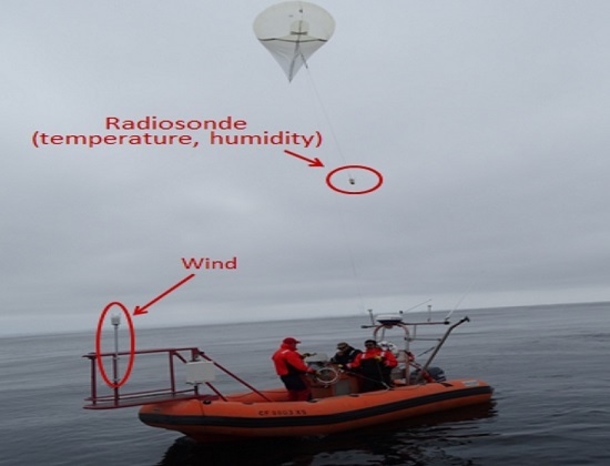
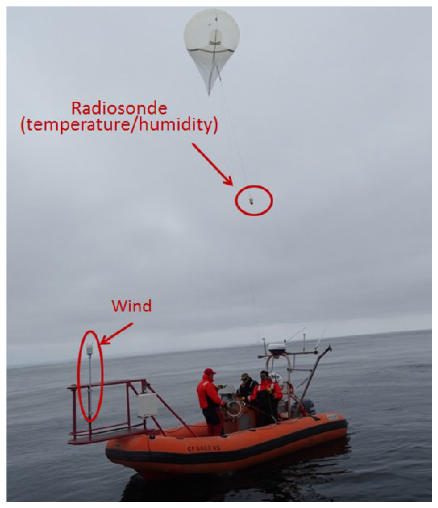
2.2. The Testing Data Sets

2.3. Optimal Estimation Based on the Weighted Nonlinear Least-Squares
2.4. The Numerical Algorithm
3. Results and Discussions
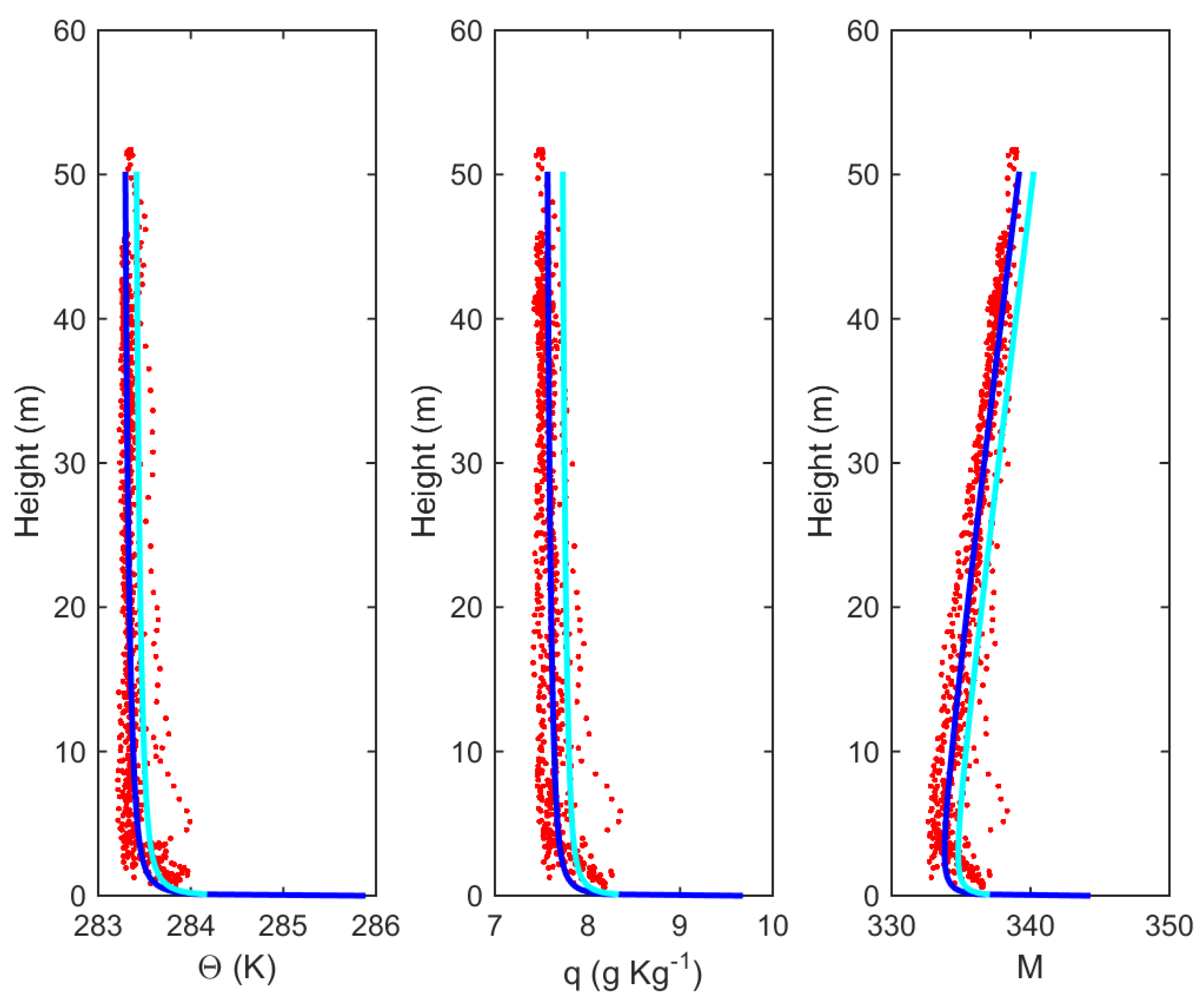
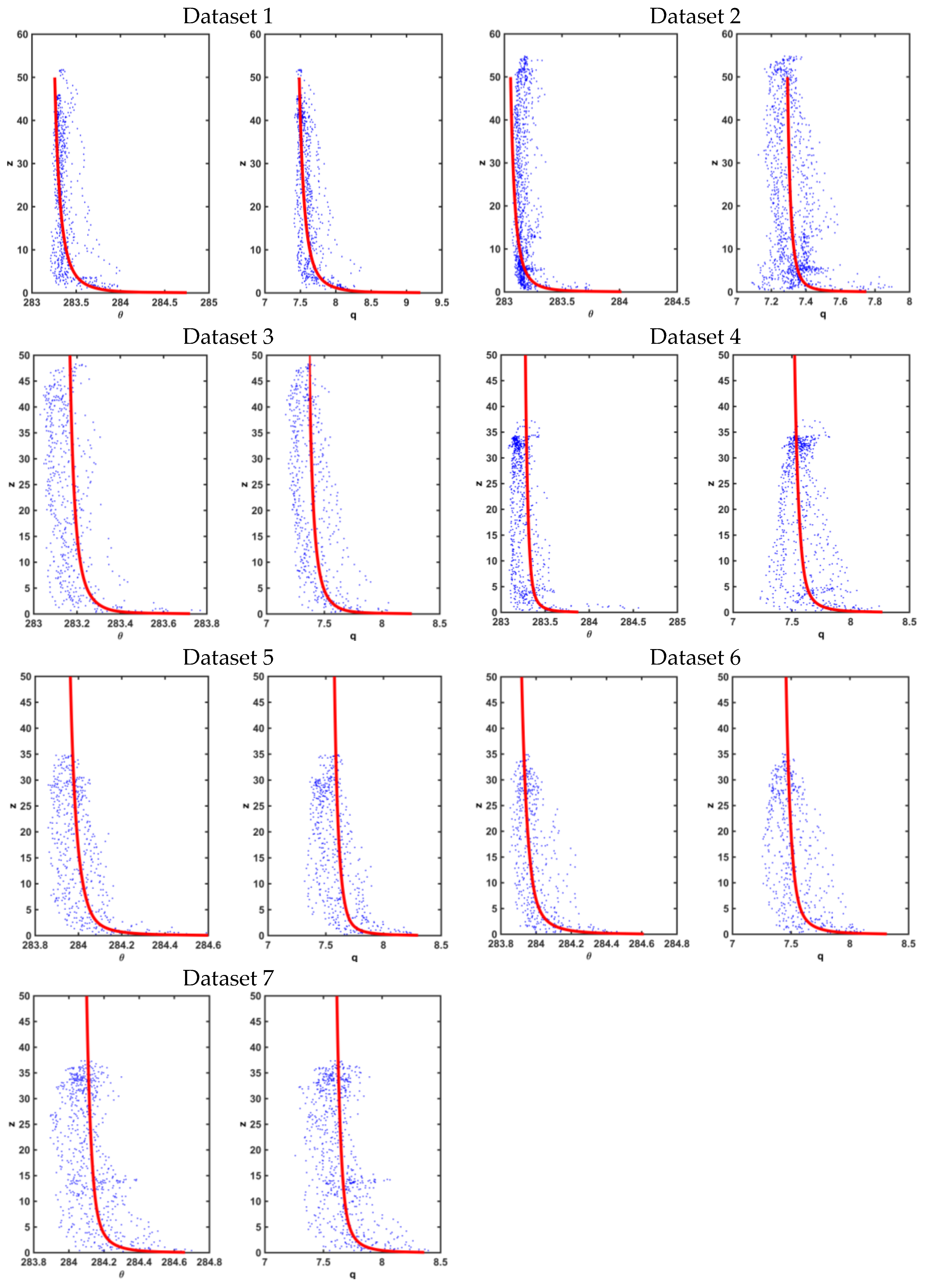
3.1. Estimated Surface Layer Profiles and Fluxes

| -- | Cost | Momentum Flux | Sensible Heat Flux | Latent Heat Flux | |||
|---|---|---|---|---|---|---|---|
| Data 1 | 0.47 | 0.12 | −0.340 | −0.391 | −0.018 | 52.61 | 150.15 |
| Data 2 | 1.07 | 0.06 | −0.454 | −0.215 | −0.005 | 35.02 | 41.28 |
| Data 3 | 0.69 | 0.10 | −0.096 | −0.154 | −0.014 | 12.78 | 50.97 |
| Data 4 | 0.99 | 0.19 | −0.056 | −0.069 | −0.044 | 13.38 | 41.39 |
| Data 5 | 0.82 | 0.16 | −0.067 | −0.076 | −0.034 | 14.17 | 40.08 |
| Data 6 | 0.81 | 0.20 | −0.062 | −0.077 | −0.053 | 16.36 | 50.41 |
| Data 7 | 0.70 | 0.20 | −0.048 | −0.064 | −0.052 | 12.51 | 41.46 |

3.2. Choice of Weights and the Cost Function
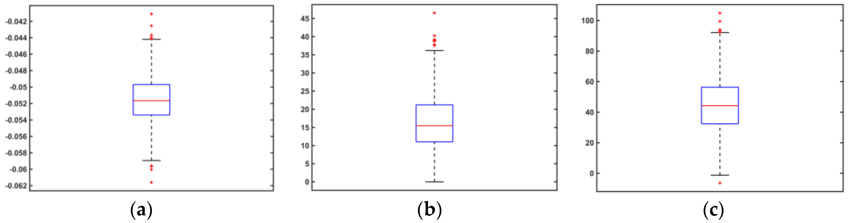
3.3. The Characteristics of the Estimator—An Empirical Analysis
| -- | True Value | Mean | Median | Standard Deviation | IQR | Maximum | Minimum |
|---|---|---|---|---|---|---|---|
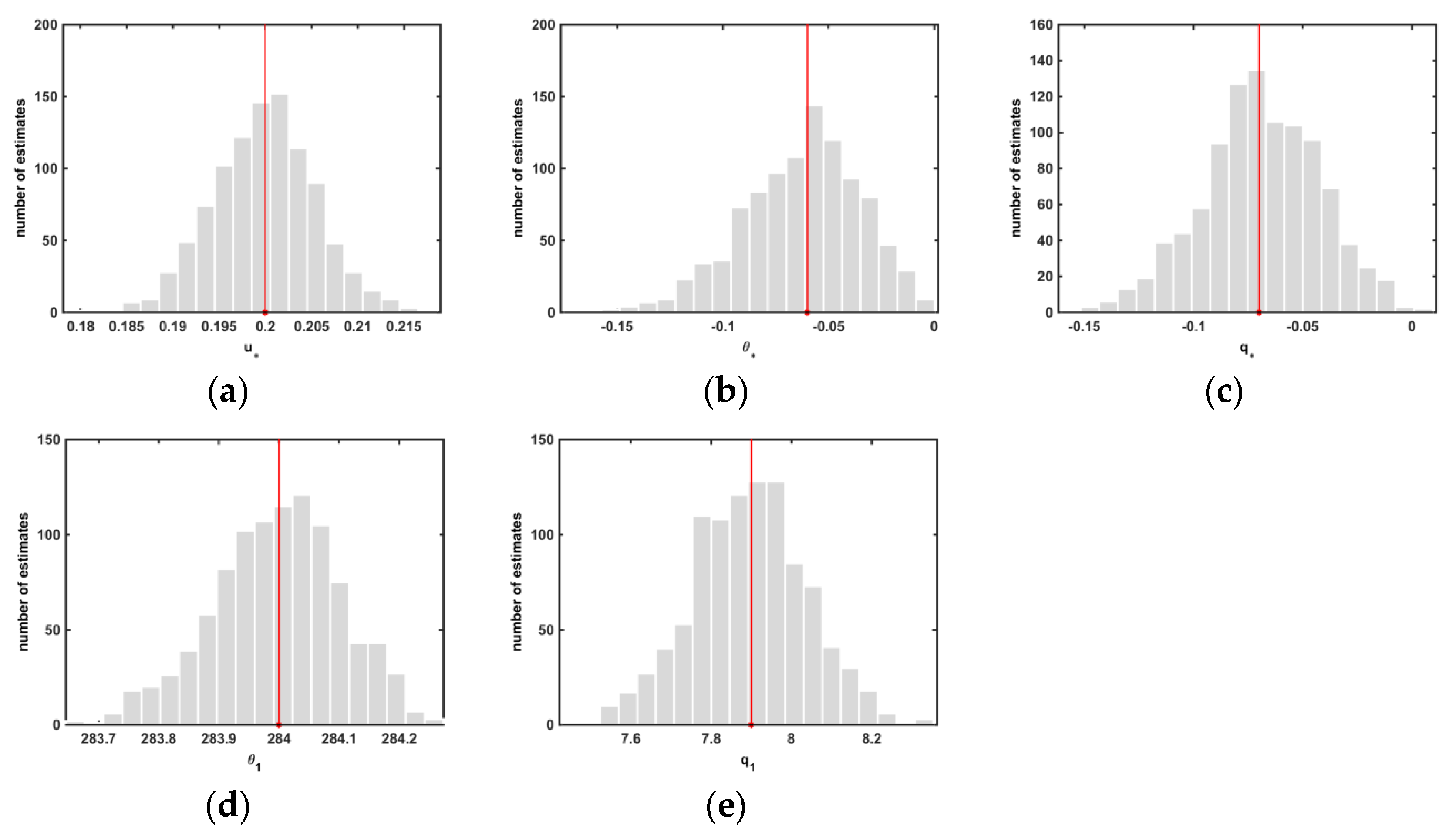
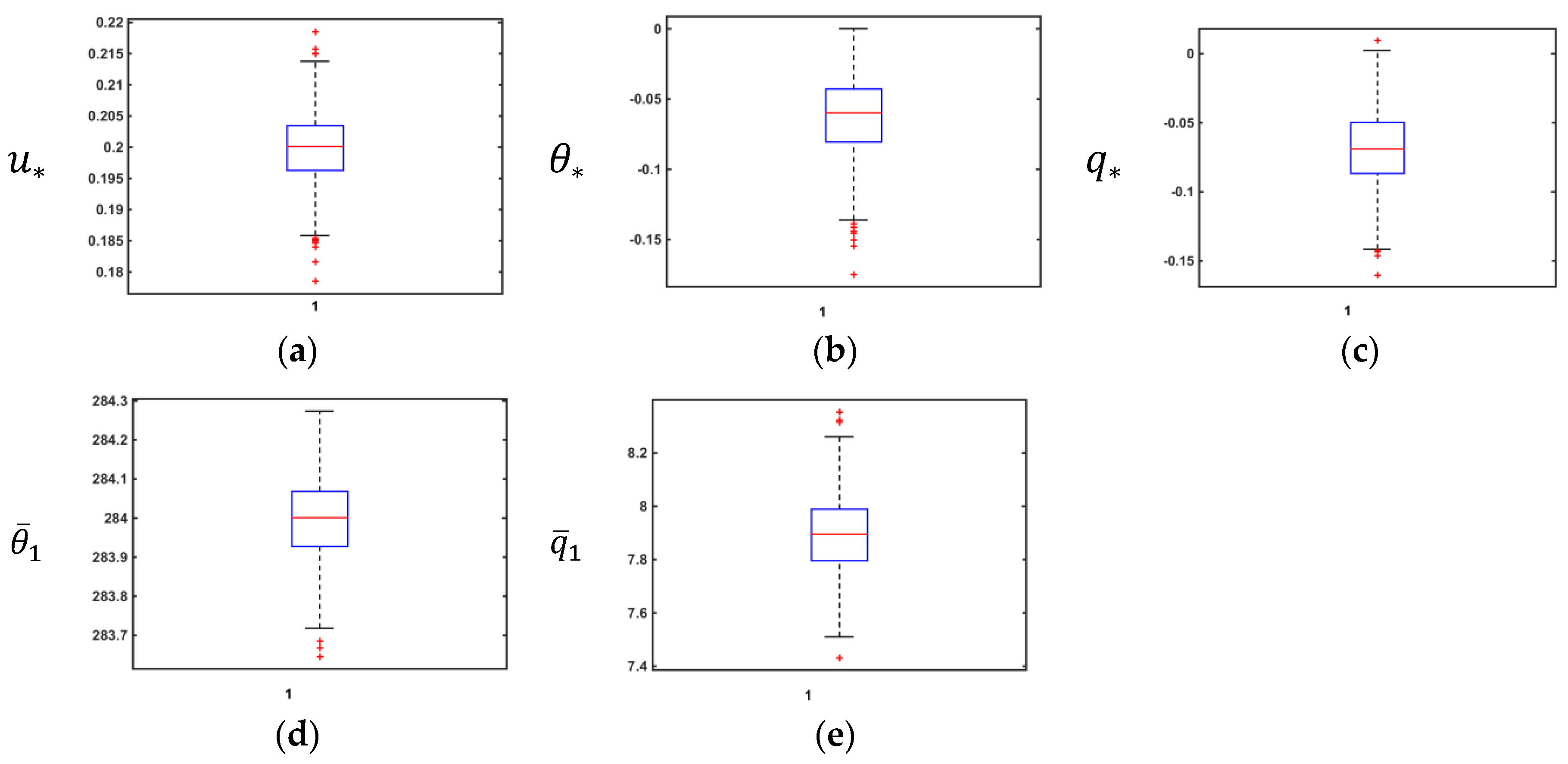
| 0.20 | 0.20 | 0.20 | 5.52 × 10⁻³ | 7.18 × 10⁻³ | 0.22 | 0.18 | |
| –0.06 | –0.06 | −0.06 | 0.028 | 0.038 | 8.0 × 10⁻⁵ | −0.175 | |
| –0.070 | –0.069 | −0.069 | 0.027 | 0.037 | 9.45 × 10⁻³ | −0.016 | |
| 284.00 | 284.00 | 284.00 | 0.106 | 0.141 | 284.27 | 283.66 | |
| 7.90 | 7.89 | 7.90 | 0.014 | 0.019 | 8.35 | 7.74 |
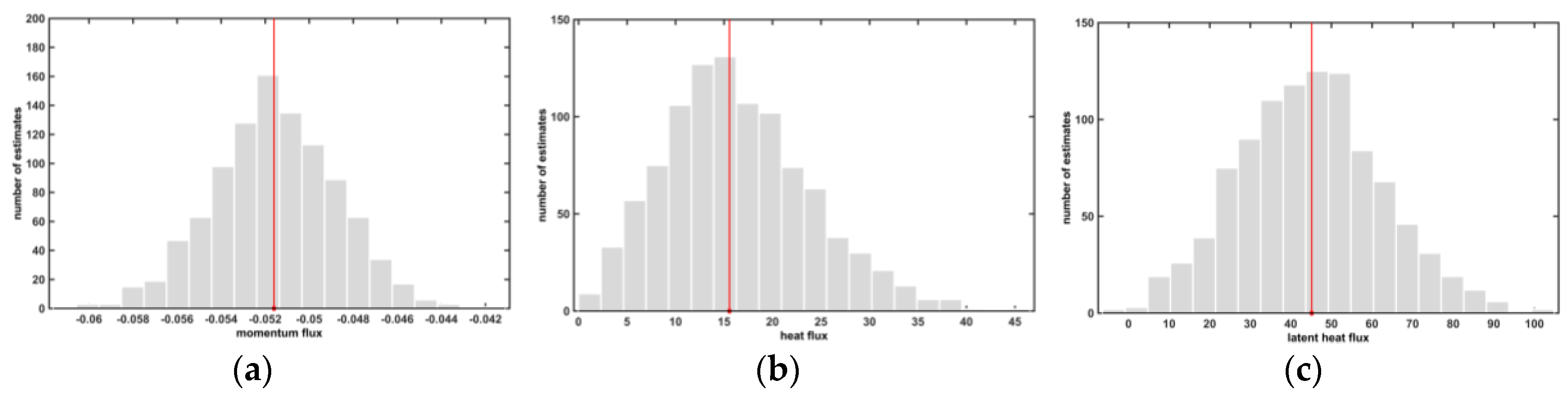
| -- | True Value | Mean | Median | Std dev | IQR | Maximum | Minimum |
|---|---|---|---|---|---|---|---|
| Momentum Flux | −0.052 | −0.052 | −0.052 | 2.84 × 10⁻³ | 3.70 × 10⁻³ | −0.041 | −0.062 |
| Sensible Heat Flux | 15.56 | 16.36 | 15.46 | 7.46 | 10.18 | 46.52 | −0.02 |
| Latent Heat Flux | 45.15 | 44.61 | 44.2 | 17.63 | 23.93 | 104.85 | −6.37 |

4. Discussion and Conclusions
Acknowledgments
Author Contributions
Conflicts of Interest
References
- Webster, P.J.; Lukas, R. The coupled ocean atmosphere response experiment. Bull. Am. Meteorol. Soc. 1992, 73, 1377–1416. [Google Scholar]
- Turton, J.D.; Bennets, D.A.; Farmer, S.F.G. An introduction to radio ducting. Meteorol. Mag. 1988, 117, 245–254. [Google Scholar]
- Babin, S.M.; Young, G.S.; Carton, J.A. A new model of the oceanic evaporation duct. J. Appl. Meteorol. 1997, 36, 193–204. [Google Scholar] [CrossRef]
- Paulus, R.A. Practical application of an evaporation duct model. Radio Sci. 1985, 20, 887–896. [Google Scholar] [CrossRef]
- Anderson, K.; Brooks, B.; Caffrey, P.; Clarke, A.; Cohen, L.; Crahan, K.; Davidson, K.; de Jong, A.; de Leeuw, G.; Dion, D.; et al. The RED experiment, an assessment of boundary layer effects in a trade wind regime on microwave and infrared propagation over the sea. Bull. Am. Meteorol. Soc. 2004, 85, 1355–1365. [Google Scholar] [CrossRef]
- Edson, J.B.; Zappa, C.J.; Ware, J.A.; McGillis, W.R. Scalar flux profile relationship over the open ocean. J. Geophys. Res. 2004, 109. [Google Scholar] [CrossRef]
- Fairall, C.W.; Bradley, E.F.; Hare, J.E.; Grachev, A.A.; Edson, J.B. Bulk parameterization of air-sea fluxes: Updates and verification for the COARE algorithm. J. Clim. 2003, 16, 571–591. [Google Scholar] [CrossRef]
- Businger, J.A.; Wyngaard, J.C.; Izumi, Y.; Bradley, E.F. Flux profile relationship in the atmospheric surface layer. J. Atmos. Sci. 1971, 28, 181–189. [Google Scholar] [CrossRef]
- Nieuwstadt, F. The computation of the friction velocity and the temperature scale from temperature and wind velocity profiles by least-square methods. Bound.-Layer Meteorol. 1978, 14, 235–246. [Google Scholar] [CrossRef]
- Kramm, G. The estimation of the surface-layer parameters from wind velocity, temperature and humidity profiles by least-squares methods. Bound.-Layer Meteorol. 1989, 48, 315–327. [Google Scholar] [CrossRef]
- Fairall, C.W.; Bradley, E.F.; Rogers, D.P.; Edson, J.B.; Young, G.S. Bulk parameterization of air-sea fluxes in TOGA COARE. J. Geophys. Res. 1996, 101, 3747–3767. [Google Scholar] [CrossRef]
- Panofsky, H.A. Determination of stress from wind and temperature measurements. Q. J. R. Meteorol. Soc. 1963, 89, 85–94. [Google Scholar] [CrossRef]
- Charnock, H. Wind stress on a water surface. Q. J. R. Meteorol. Soc. 1955, 81, 639–640. [Google Scholar] [CrossRef]
- Liu, W.T.; Katsaros, K.B.; Businger, J.A. Bulk parameterization of the air-sea exchange of heat and water vapor including the molecular constraints at the interface. J. Atmos. Sci. 1979, 36, 1722–1735. [Google Scholar] [CrossRef]
- Grachev, A.A.; Fairall, C.W.; Bradley, E.F. Convective profile constants revisited. Bound.-Layer Meteorol. 2000, 94, 495–515. [Google Scholar] [CrossRef]
- Gill, P.E.; Murray, W.; Wright, M.H. Practical Optimization; Academic Press, INC.: London, UK, 1981. [Google Scholar]
- Van de Geer, S.A. Least square estimation. In Encyclopedia of Statistics in Behavioral Science; John Wiley & Sons, Ltd: Chichester, UK, 2005. [Google Scholar]
- Hock, T.F.; Franklin, J.L. The NCAR GPS Dropwindsonde. Bull. Am. Meteorol. Soc. 1999, 80, 407–420. [Google Scholar] [CrossRef]
- Powell, M.D.; Vickery, P.J.; Reinhold, T.A. Reduced drag coefficient for high wind speeds in tropical cyclones. Nature 2003, 422, 279–283. [Google Scholar] [CrossRef] [PubMed]
- Godfrey, J.S.; Beljaars, A.C.M. On the Turbulent Fluxes of Buoyancy, Heat, and Moisture at the Air-Sea Interface at Low Wind Speeds. J. Geophys. Res. 1996, 96, 22043–22048. [Google Scholar] [CrossRef]
- Janssen, P.A.E.M. The Interaction of Ocean Waves and Wind; Cambridge University Press: Cambridge, UK, 2004; p. 308. [Google Scholar]
- Grachev, A.A.; Fairall, C.W.; Hare, J.E.; Edson, J.B.; Miller, S.D. Wind stress vector over ocean waves. J. Phys. Oceanogr. 2003, 33, 2408–2429. [Google Scholar] [CrossRef]
- Fairall, C.W.; Bariteau, L.; Grachev, A.A.; Hill, R.J.; Wolfe, D.E.; Brewer, W.A.; Tucker, S.C.; Hare, J.E.; Angevine, W.M. Turbulent bulk transfer coefficients and ozone deposition velocity in the International Consortium for Atmospheric Research into Transport and Transformation. J. Geophys. Res. 2006, 111, D23S20. [Google Scholar] [CrossRef]
© 2016 by the authors; licensee MDPI, Basel, Switzerland. This article is an open access article distributed under the terms and conditions of the Creative Commons by Attribution (CC-BY) license (http://creativecommons.org/licenses/by/4.0/).
Share and Cite
Kang, D.; Wang, Q. Optimized Estimation of Surface Layer Characteristics from Profiling Measurements. Atmosphere 2016, 7, 14. https://doi.org/10.3390/atmos7020014
Kang D, Wang Q. Optimized Estimation of Surface Layer Characteristics from Profiling Measurements. Atmosphere. 2016; 7(2):14. https://doi.org/10.3390/atmos7020014
Chicago/Turabian StyleKang, Doreene, and Qing Wang. 2016. "Optimized Estimation of Surface Layer Characteristics from Profiling Measurements" Atmosphere 7, no. 2: 14. https://doi.org/10.3390/atmos7020014
APA StyleKang, D., & Wang, Q. (2016). Optimized Estimation of Surface Layer Characteristics from Profiling Measurements. Atmosphere, 7(2), 14. https://doi.org/10.3390/atmos7020014