Abstract
Due to the chaotic nature of atmospheric dispersion, small deviations, e.g., numerical errors in dispersion simulations, increase rapidly over time. Therefore, the accuracy of backward simulations is limited. In the paper, the degree of the fulfillment of time-reversibility over different time periods is investigated by a Lagrangian dispersion model at a global scale using pollutant clouds consisting of a large number of particles. The characteristics of the pollutant clouds in the backward simulation are compared to those in the forward simulation. In order to characterize the degree of time-reversibility, Lagrangian quantities, such as the fraction of particles that return to the initial volume, the center of mass and the standard deviation of the pollutant clouds, are determined. Furthermore, the overlap and the Pearson’s correlation coefficient between the forward and backward clouds are also investigated. Both a case study and global results are presented. Simulations reveal that the accuracy of time-reversibility decreases in general exponentially in time. We find that after the Lyapunov time of the dispersion (in our case three to four days), the results of the backward tracking become unreliable, and any sign of time-reversibility is lost.
“When you stir your rice pudding, Septimus, the spoonful of jam spreads itself round making red trails like the picture of a meteor in my astronomical atlas. But if you stir backwards, the jam will not come together again. Indeed, the pudding does not notice and continues to turn pink just as before. Do you think this is odd?”Tom Stoppard: Arcadia
1. Introduction
Backward calculation of the transport and dispersion in the atmosphere is a tool commonly used for identifying the sources of pollutants or other substances and/or to provide a dispersion model with input data optimized to all of the knowledge exploited from available measurements for future studies. Besides simple trajectory computation (see, e.g., [1]), more sophisticated techniques exist to estimate the location and distribution of substances at a certain time before the observation. These methods are described in detail in [2] and the references therein, including inverse modeling using a source-receptor relationship by means of a Lagrangian model [3] and adjoint versions of Eulerian dispersion models [4,5].
In this study, we focus on the degree at which the time-reversibility property is fulfilled in backward tracking of individual pollutant particles. For the investigation, we use a Lagrangian trajectory model applied in many research areas in meteorology, including calculation of the origin of particulate matter [6,7], pollen [8,9], moisture [10,11] or gases and passive tracers [12,13,14]. In the simplest case, when only advection is taken into account, particle trajectories are determined utilizing 3D velocity fields of the atmosphere, and the motion of the particles is deterministic and described by three time-dependent differential equations in the horizontal and vertical directions.
In deterministic dynamical systems, the naive expectation suggests that if the system develops for a certain time forward, then time is reversed, and if the evolution of the system is followed backwards for the same time period, the initial state should be recovered. This is expected to hold in simple dynamical systems rather accurately, even if the development of the system is determined numerically.
However, if the deterministic dynamical system is nonlinear and is described by at least three first-order autonomous differential equations (or by two time-dependent differential equations), chaotic behavior can appear [15,16,17], the typical characteristics of which are sensitivity to initial conditions, irregular motion and the appearance of complex formations, like folded, elongated filaments and tendrils [18]. Three-dimensional passive advection has three degrees of freedom, that is advection dynamics can result in chaotic motion even if the flow field by which the particles are advected is smooth and deterministic. The characteristics of chaos were also experienced in atmospheric dispersion problems of contaminants (see, e.g., [19,20,21]).
Chaotic behavior is the reason for the fact that the motion of a particle is unpredictable for long times as the trajectories of initially nearby particles diverge in an exponential manner. Small differences in the initial position and numerical approximations used in the calculation induce errors growing exponentially in time. In view of the sensitivity to slight deviations, instead of one trajectory, several adjacent particles should be tracked to get a more precise overview of the volume/area covered potentially by the contaminant.
In the dynamical systems literature, the breakdown of time-reversibility in chaotic systems due to the unavoidable numerical errors was first pointed out by Shepelyansky [22]. An illustrative example with an ensemble of particles in an elementary problem is given in the textbook [17].
In this paper, we investigate the accuracy of backward trajectory simulations in atmospheric dispersion as a function of time and, thereby, the degree of the fulfillment of time-reversibility in the view of chaotic advection. As a first step, a forward trajectory simulation of a pollutant cloud consisting of several particles emitted instantaneously is carried out for a maximum of nine days using a Lagrangian trajectory model. Figure 1 provides a first insight into the basic phenomenon. The black dots in Figure 1b trace out the position of an initially localized particle cloud for time instant days. Particles correspond to passive tracers, that is they represent solid or liquid contaminants of negligible size or a gaseous contaminant. The location of the pollutant clouds of the forward run started at day serves as a reference for the succeeding backward simulations. Backward simulations start at days from the particle distribution of the forward simulation at as the initial condition and track back the particles till (see the colored dots in Figure 1a). For clarity, an outline of the time schedule of the forward and backward simulations is given in Figure 2. In general, the accuracy of backward tracking as a function of the time interval of the backward simulation is assessed by comparing the forward cloud and the backward clouds at time instants days. For example, we compare the forward cloud with nine backward clouds at , three of which are illustrated in Figure 1a, and with two backward clouds at days, only one of which is represented in Figure 1b for better visibility, respectively. In this way, the “exact” initial conditions of the backward simulations at time are known within the rounding-off error of the computer. The forward pollutant cloud at time t is considered to be the “original” position of the particles where the particles should return. The deviations between the backward cloud and forward cloud are caused by the rounding-off errors and errors of the numerical scheme for integration of the equation of motion. These errors are amplified over time due to chaoticity. Figure 1 shows that the longer the time interval of the backward tracking, the worse the coincidence between the forward and backward clouds, e.g., the bad agreement of the forward and backward cloud can be illustrated by the red dots with days of backward tracking in Figure 1a spreading from Asia to Europe, while the blue dots in Figure 1a and the red dots in Figure 1b both with days of backward tracking are in reasonable agreement with the corresponding forward clouds (denoted by black dots), respectively.
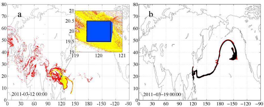
Figure 1.
Forward (black) and backward (colored) pollutant clouds emitted instantaneously and consisting of particles at (a) and (b) days. The forward pollutant cloud is initiated on 12 March 2011 at 00 UTC at E, N, 500 hPa in a hPa cuboid beyond Indonesia. Colored dots denote the location of the particles whose backward simulation started at time days (blue), days (yellow) and days (red), respectively. In the inset of panel (a) instead of black dots the initial position of the particles is illustrated by a black rectangular frame. This simulation is an element of the global study in Section 6.
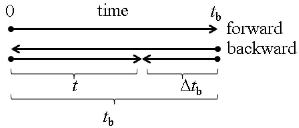
Figure 2.
An outline of the time schedule of the forward and backward simulations. Forward simulation starts at Time 0 and terminates after nine days. Backward simulations start at time (where the value of can be days) and terminate at Time 0. The comparison of the forward and backward cloud is carried out at time t ( days) as a function of the time period of the backward tracking.
In order to analyze the matching of the appropriate backward and forward clouds, statistical parameters are determined. We investigate Lagrangian quantities, which depend solely on the position of the particles, and Eulerian ones, which require the particles to be projected into grid cells. In this way, the proportion of the particles returned back to the initial volume of the cloud is determined, as well as some parameters already applied in earlier studies [23,24]. These quantities are the difference between the center of mass of the backward and forward pollutant clouds, the difference between the standard deviations of the particles in the clouds and the overlap and Pearson’s correlation coefficient of the two clouds. The paper presents a case study and, furthermore, simulations distributed uniformly over the globe to get a general overview of the behavior of the statistical parameters. As a general rule, parameters reveal that the accuracy of backward tracking decreases exponentially in time, and usually after a few days or about a week, the results of the backward tracking become unreliable; any sign of time-reversibility is lost.
The paper is organized as follows. Section 2 provides a brief overview of the RePLaT model by which the particle trajectories are monitored. Section 3 describes the meteorological data used for the simulations and the initial distribution of the pollutants, while Section 4 introduces the statistical parameters applied for the characterization of the accuracy of backward simulations. The results of a case study and global studies are presented in Section 5 and Section 6, respectively. An outlook is given in Section 7, and Section 8 summarizes the conclusions of the work.
2. The RePLaT Dispersion Model
The RePLaT (Real Particle Lagrangian Trajectory) dispersion model, first formulated in [25], is used to calculate the trajectories of particles that compose the pollutant clouds. RePLaT is a Lagrangian model tracking aerosol particles with a realistic radius and density. Ideal tracers and gaseous contaminants correspond to particles with radius . RePLaT is applied here in this limiting case. Although there exist a few Lagrangian trajectory models where the advection of a particle is determined by higher order integration schemes (e.g., TRAJ3D [26]), in most cases, this process is computed by integrating the equation of motion by using Euler’s method (NAME [27], MLDP0 [28], SNAP [29], GEARN [30]) or second-order methods (FLEXPART [31], HYSPLIT [32]). RePLaT also calculates particle trajectories by means of the forward Euler’s method:
where indicates the particle position at time t, is the wind speed vector at the location of the particle and is the time step. In forward simulations, , while in backward simulations, . Since after a few days a particle cloud traces out the unstable foliation of a chaotic dynamics, the shape of this pattern is expected to be insensitive to the choice of the numerical code. The reason is that exponential divergence occurs along the unstable foliation only; in the perpendicular directions exponential contraction occurs, just like for chaotic attractors [17]. Any numerical algorithm is thus able to easily converge to the unstable foliation. Where unpredictability plays a role is the position of a given trajectory endpoint along the unstable foliation; this, however, is not an issue in our simulations, since instead of individual trajectories, an ensemble is treated.
RePLaT also reckons with the impact of turbulent diffusion on the particles as a random walk process, and the use of Euler’s method is motivated by an easy treatment of this part of the code. However, since in large-scale simulations, its effect is much weaker than that of advection [19], as a first approximation, turbulent diffusion is neglected in the simulations. Turbulent diffusion will only be treated in Section 7.
In the present study, if an ideal tracer particle encounters the surface, it bounces back to the atmosphere with a perfectly elastic collision.
In order to calculate the trajectories of the particles using Equation (1), meteorological data given on a regular grid are interpolated to the position of the particles (using bicubic spline interpolation in the horizontal direction and linear interpolation in the vertical direction and in time). For more details about RePLaT, see [25].
3. Input Data
The particle trajectories are computed using the reanalysis fields of the ERA-Interim database of the European Centre for Medium-Range Weather Forecasts (ECMWF) [33], where u and v are the longitudinal and latitudinal velocity component of air, respectively, and ω is the vertical velocity in pressure coordinates. The meteorological variables utilized in the simulations are given on 32 pressure levels between 1000 and 100 hPa on a horizontal grid with 6 h of time resolution.
The time step of the simulation is determined by the inequality , where , and are the resolution of the grid of the meteorological data [34]. Based on this relation, the time step is chosen to be min.
The time interval of particle tracking in both the case study and the global simulations is at most nine days beginning on 12 March 2011 at 00 UTC. The particles in the forward simulations are emitted instantaneously in the atmosphere at this time instant.
In the case study (Section 5), particles are initially distributed uniformly in a hPa volume centered at E, N, hPa. It can be considered as a hypothetical sudden emission over Fukushima occurred on 12 March 2011 at 00 UTC, however, well above the real emission. We chose the time period because of the well-documented meteorological situation (see, e.g., [35]), but particles are placed higher in the atmosphere in order to be able to investigate the transport on large scales.
In the global simulation (Section 6), the initial position of the pollutant clouds is of the same size at the same altitude as in the case study. From W to E in increments and S to N in increments, pollutant clouds are emitted instantaneously at the time mentioned above on a “grid” in the atmosphere. The results of Figure 1 arise from an instantaneous injection in one of these grid points.
4. Statistical Parameters
In order to quantify the accuracy of the backward simulation, the pollutant clouds of the backward and forward simulations at the appropriate time instants are compared using different statistical quantities, which are detailed in the subsequent subsections. The proportion of the particles that returned to the initial volume, the deviation of the center of mass and the difference of the standard deviation of the pollutant clouds are solely based on the position of the particles, while the figure of merit in space (overlap) and the Pearson’s correlation coefficient (suggested by, e.g., [24]) demand the use of an artificial grid over which concentration can be calculated.
The differences between the backward and forward pollutant clouds (BWC and FWC) are considered as a function of the time interval of the backward simulation , where is the initialization time of the backward simulation ( days) and t is the time instant of the comparison ( days). Since we have backward simulations beginning at days, e.g., for day, nine values are available for each measure (except for ), because the BWC with day can be compared to the FWC at , the one with days at day, and so on. Therefore, for days, we have only one value, since only the backward cloud with days can be compared to the forward cloud at .
4.1. Proportion of Particles Returned to the Initial Volume
For each , the number n of the particles that returned to the initial hPa volume is determined. The proportion describes how accurately a backward simulation of can track back the pollutant cloud to the source.
4.2. Center of Mass and Standard Deviation of the Pollutant Clouds
The horizontal coordinates of the center of mass and of the FWC and BWCs and the standard deviation and of the particles in the clouds are calculated at days, and the deviation between the backward and forward simulations is determined. In order to eliminate the effect of the convergence of meridians, and are not computed by averaging the longitudinal and latitudinal coordinates of the particles, but by converting their position to 3D Cartesian coordinates before averaging ( being the center of the Earth). The averaged coordinates are projected back to the surface of the Earth in latitude-longitude coordinates. The standard deviation of the particles in the clouds and the differences between the center of masses of the BWCs and FWC are calculated using spherical distances:
where are the latitudinal and longitudinal coordinates of the i-th particle in the cloud studied and , and , are the same for the center of mass of the FWC and BWC, respectively. The spherical distance between two locations given by latitudinal and longitudinal coordinates is traditionally given in radians [36]. In order to represent it in kilometers, radians are changed to degrees (multiplication by ), and then, they are multiplied by , the average length of one degree on the surface of the globe.
The difference between the center of masses characterizes the average shift between the FWC and BWC, while the difference between the standard deviations describes the typical difference in the extension of the BWC and FWC.
4.3. Figure of Merit in Space
The percentage of overlap (called the figure of merit in space) between the BWC and FWC is also calculated. It is defined as the ratio between the intersection and the union of the two pollutant clouds [24]. Besides the conventional 2D overlap (i.e., overlap of air columns), the 3D overlap is also determined in the study:
where and are the area and volume of the backward pollutant clouds, respectively, and and correspond to those of the forward clouds. If , there is an exact overlap between the two clouds, that is . When , the BWC and FWC do not cover each other completely due to their different shape and/or shift following from their different location.
As RePLaT tracks individual particles, in order to estimate , and , particles need to be projected onto a grid. In the horizontal direction, instead of the obvious regular longitudinal-latitudinal grid, we use a modified grid detailed in [19] in order to eliminate a strange feature of the regular grid, namely that a cell of has a much smaller area close to the poles than near the Equator. In the modified grid, the latitudinal side of a cell is equal at any latitude, and the longitudinal size changes depending on the latitude, so that the area of the cells is almost equal. In this paper, , and , denote the number of such cells with at least one particle. Note that in the value of and , rarely occupied cells are over-weighted, since a cell consisting of only one particle is taken into account with exactly the same weight as a cell with a large number of particles.
4.4. Pearson’s Correlation Coefficient
Pearson’s correlation coefficient [24] is also determined for air columns () and for air volumes () to study whether the backward and forward clouds are correlated in space. The is defined as:
where K is the number of 2D or 3D cells where the backward and/or forward clouds are present (here, cells to which at least one particle belongs), is the number concentration (the number of particles in the cell divided by ) of the backward/forward cloud in cell i and is the mean concentration of the backward/forward cloud.
5. Case Study
In order to study the accuracy of time-reversibility in the dispersion of pollutant clouds with deterministic Equation (1), as a first exercise, a forward simulation of nine days and the corresponding backward simulations are carried out. The particles of the FWC are initiated in a volume of hPa at the time and location mentioned in Section 3. Figure 3 illustrates the FWC (black) and the BWCs (colored) at and 2, 5 and 7 days after the emission.
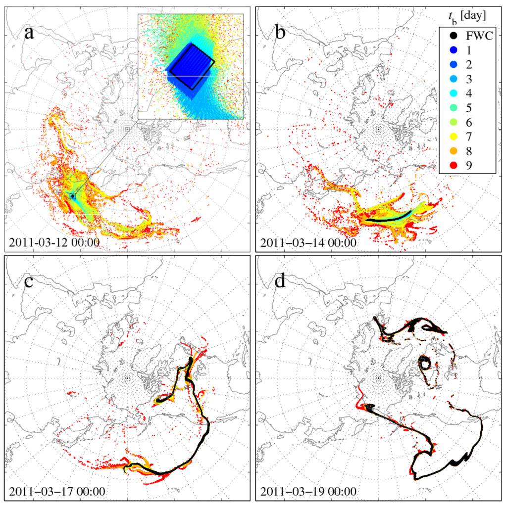
Figure 3.
Forward (black) and backward (colored) pollutant clouds emitted instantaneously and consisting of particles of the case study at (a) , (b) , (c) and (d) days. The forward pollutant cloud is initiated on 12 March 2011 at 00 UTC at E, N, 500 hPa in a hPa cuboid beyond Fukushima. Dots colored according to the color bar on the right denote the location of the particles whose backward simulation started at time (day). In the inset of panel (a), instead of black dots, the initial position of the particles is illustrated by a black rectangular frame. For better visibility, only every fifth particle of the clouds is plotted.
The meteorological situation during the studied days is detailed, e.g., in [35]. The black FWC leaves Japan eastwards with the strong flow of a jet, while due to the shearing in the wind field, it stretches more and more. On 15 March (not shown in Figure 3), the elongated filament gets into a flow region dominated by a cyclone at the western coast of North America due to which it begins to form a spiral. Some days later, as was also experienced in the case of the real emission from Fukushima, some fraction of the FWC reaches Europe. The complex, folded and rather stretched shape of the initially compact pollutant cloud is the consequence of the chaotic nature of the advection mentioned in the Introduction.
A fairly good agreement and almost total overlap appear on 12 March between the FWC and the dark blue BWC ( day, day), on 14 March for the cyan and light blue BWC ( days, days), on 17 March for the green and yellow BWC ( days, days) and on 19 March for the orange BWC ( days, day). Additionally, on 12 March, the BWC with days ( days), on 14 March, the BWC with days, on 17 March the BWC with days and on 19 March, the BWC with days ( days in these cases) do not differ too much from the corresponding FWC either. The observation suggests that for –3 days, the backward simulations provide reasonable agreement, with the FWCs considered here as the “measured” position of the pollutants. For larger values of , however, the agreement is poor, and a clear breakdown of time-reversibility is found.
The agreement of the FWC and BWCs can be also studied not only by the naked eye, but in a quantitative way. In Figure 4, the example of the horizontal standard deviation and of the clouds are shown. Figure 4a reveals that after a few days of exponential growth (the exponent is day), exhibits a power-law behavior with an exponent of . The crossover between an initially exponential growth to a power-law is a general observation of studies of chaotic advection [37]. The crossover is set by the largest characteristic size of the flow, beyond which particles carry out a random walk in-between these large-scale structures. In our case, this size is that of the cyclones, and indeed, is on the order of 1000 km when the crossover takes place. The value of exponent γ is also in harmony with previous studies; see, e.g., [38]. Huber et al. experienced superdiffusivity (roughly ballistic dispersion) in mid- and high latitudes on time-scales of 10 days and found that in some mid-latitudinal locations, an exponential growth for short time intervals was present. Figure 4b shows the dependence of on the time interval of the backward simulation . That is, the data in Figure 4a are projected to the vertical axis of Figure 4b, because they are the initial conditions of the backward simulations with . Dashed lines connect the values corresponding to the time instants t when the properties of the FWC and BWCs are going to be compared. One can see that in the first 3–4 days of the backward simulations, decreases in a similar manner as increases in the forward mode. The almost horizontal nature of the dashed lines show that the values of are close to . Later, however, the decrease slows down, and within 5–6 days, it switches to an increase again. This increase is a clear sign of irreversibility.
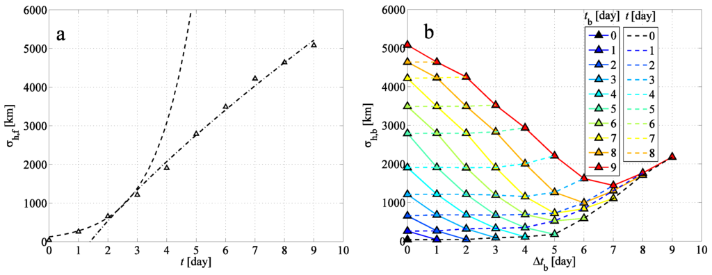
Figure 4.
(a) The horizontal standard deviation of the forward cloud (FWC) in Figure 3 as a function of time t with an exponential fit over –2 days (dashed line) and a power-law fit over –9 days (dash-dotted line); (b) the horizontal standard deviation of the backward clouds (BWCs) in Figure 3 as a function of the time interval of the backward simulation . Solid lines represent the time evolution of the BWCs initiated at (see color legend) backward in time; dashed lines connect the values corresponding to time t.
To quantify the differences between the BWCs and FWCs, the statistical parameters introduced in Section 4 are calculated. Figure 5 illustrates the Lagrangian ones when the calculation is based only on the position of the particles.
The horizontal distance between the center of mass of the FWC and the BWCs increases as a function of . The chaotic nature of the advection in the atmosphere implies that initially close particle pairs move away from each other exponentially. Therefore, the naive expectation emerges that the difference between the center of mass of the FWC and the BWCs can be described by an exponential function, as well. Figure 5a confirms this behavior: the mean data indeed seem to fit well to an exponential function with day. The reason of the presence of term is that in this way, the curve has to go through , as is expected for . The BWCs with of warm colors (larger ) usually perform worse than the others. This is the consequence of the fact that, e.g., for days and days (i.e., the BWC at days), the extensions of the BWC and the FWC are larger than that for or 7 days with the same ( days), and the meteorological impacts on the pollutant clouds distributed on a much wider geographical area influence the position of the center of masses more strongly. From to about five days, a widening distribution of the values of the BWCs can be seen due to the longer backward simulation. The observed distribution happens to narrow for days, since it consists of less and less data.
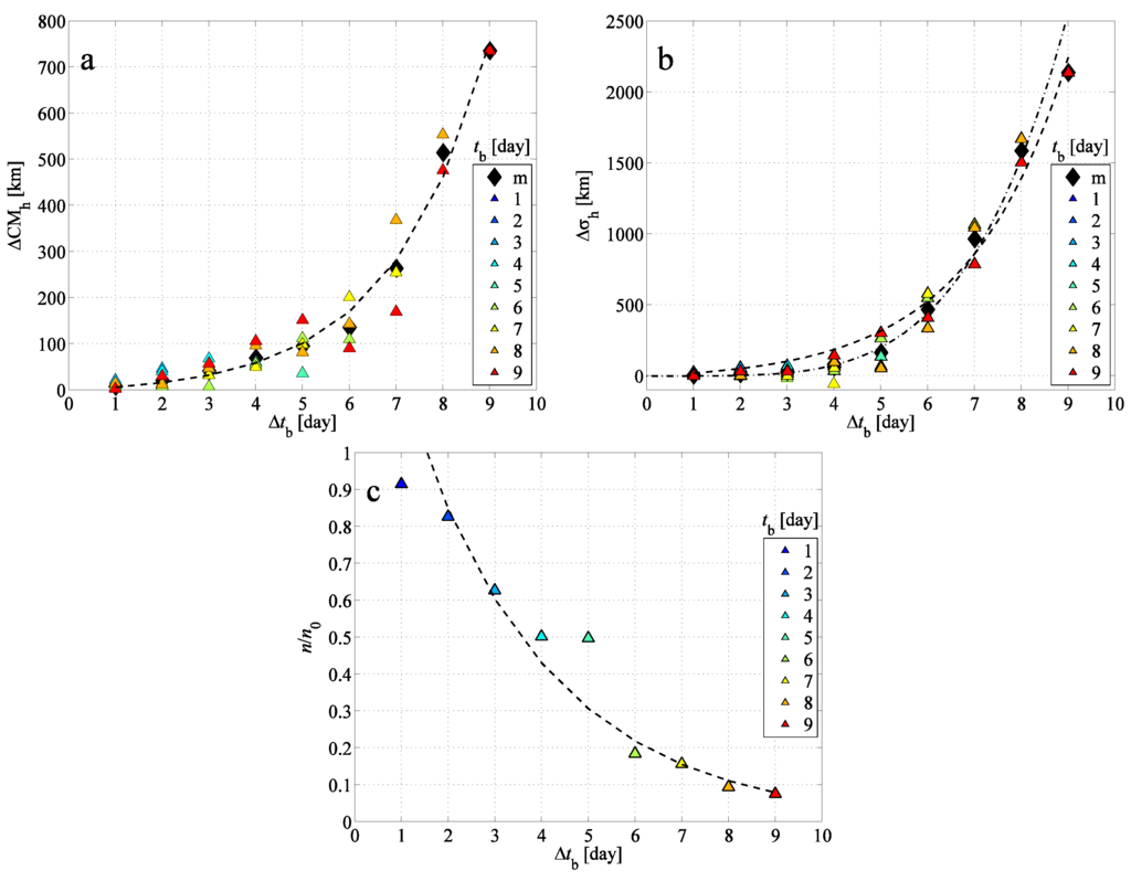
Figure 5.
(a) The horizontal difference between the center of mass of the BWCs and the FWC depending on the time period of the backward simulation; (b) the difference between the horizontal standard deviations of the BWCs and FWC; (c) the proportion of the particles returned back to the initial cuboid. Colored triangles indicate the starting time of the backward simulations (see color legend); black diamonds (in some cases in overlap with triangles) are the mean values belonging to a given (denoted by “m”). Dashed lines indicate exponential fits to the mean values; the exponents are given in Table 1. The dash-dotted line in panel (b) indicates a power-law fit to mean values over the interval –9 days with an exponent of 4.3.
Figure 5b illustrates the difference between the horizontal standard deviations of the BWCs and FWC. The panel reveals that in most cases, the BWCs cover a larger region than the corresponding FWC (). This is also a sign of the chaotic advection of the pollutant particles: small deviations grow rapidly over time (in this case, as a function of the time of backward tracking), and therefore, particles spread to a larger region than where they were at the same time instant in the FWC (see, e.g., days (red) in Figure 3). For –4 days, an exponential growth with day can be identified. Based on the characteristics of the growth in Figure 4a, over larger values, a power-law function is fitted to the mean data. However, note that we cannot expect either a clear exponential or a clear power-law behavior, since exponential and power-law regimes of and do not extend through the entire nine-day interval of investigation in . The power-law fit turns out to have an exponent of about . This γ is much larger than the γ for , which implies that an exponential fit to over the entire interval of interest might also be appropriate. The exponential function ∼ fitted to the mean data has a similar exponent as the one in the case of (see Table 1).

| - | Λ |
|---|---|
The proportion of the particles that are able to return to the inside of the initial cuboid (Figure 5c) is –0.9 for –2 days, in agreement with Figure 3a; then, it falls off quickly to 0.1 for –9 days. The decrease can again be approximated by an exponential decay: , where days. Although, the data are somewhat scattered around the exponential behavior, the type of the fit will be confirmed in the next section.
Figure 6 represents the 3D figure of merit in space and Pearson’s correlation coefficient . The resolution of the grid used for the calculation is about 20 km × 20 km × 20 hPa ( at the Equator). The alteration of the grid resolution, e.g., to , hPa, does not change the whole picture significantly, i.e., the trends and the fitted exponents are the same. Obviously, too small cells (compared to the number of released particles ) can result in “split-to-particle” clouds that have a lower chance to overlap, even if their visual expression suggests that. The limiting case is when the size of the cells tends to zero, and no overlap between the appropriate clouds can be found, since infinitely small “cells” (i.e., the individual particles) have a negligible chance to coincide. The 2D and 3D figures of merit and Pearson’s coefficients behave similarly with a shift of the measured data towards smaller values for 3D. The reason for the shift lies in that not only the horizontal, but also the vertical distribution of the clouds has to be similar. As expected, the longer the time period of the backward simulation, the worse the overlap and correlation of the BWCs and FWC. After days of backward tracking, the BWC becomes so much extended compared to the original FWC at that time that there is less than a 10% overlap between the clouds. The shift of the clouds (which is quantified in Figure 5a as ) also contributes to the lack of the coincidence of the two pollutant clouds investigated.
Although, exponential decay (∼) of the and cannot be explained directly by particle pair separation, since not only the shift and the change in extension of the clouds, but also the shape of them contribute to these quantities, Table 1 shows a reasonable agreement between the Λ of , , , and ,
Note that the exponent fitted to is 0.339, which is different from those of the other quantities. We can discover here the signature of the so-called Lyapunov exponent [16] by measuring the horizontal distance between the initial position of a particle and the position of the returned particle of the backward simulation at for all of the particles. The mean distance exhibits again an exponential growth as a function of (∼ where stands for the total time period over which the particles are advected). The Lyapunov exponent obtained this way is found to be days, which coincides reasonably well with the one obtained for . This Λ is in reasonable agreement with the atmospheric Lyapunov exponents of advection found in earlier studies (e.g., [21,39]) for a similar time span. The Λ exponents of the other statistical parameters can also be considered to be Lyapunov exponents; however, in those cases, meteorological situations of different days all contribute, the time spans are different and the contributions are thus not weighted equally. This explains why their Λ values deviate from that of . The order of magnitude of all values is a few days.
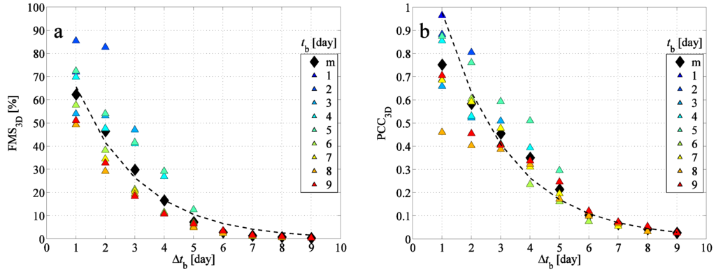
Figure 6.
(a) The figure of merit in space between the BWCs and FWC depending on the time period of the backward simulation; (b) Pearson’s correlation coefficient between the BWCs and FWC. Colored triangles indicate the starting time of the backward simulations (see the color legend); black diamonds (in some cases in overlap with triangles) are the mean values belonging to a given (denoted by “m”). Dashed lines indicate exponential fits to mean values; the exponents are given in Table 1.
Although particular values mentioned here might depend on the resolution of meteorological data used, on the interpolations applied and on the numerical scheme of the trajectory integration, one feature is independent of these details, namely that the deviation between the appropriate BWC and FWC becomes significant if the integration time exceeds the Lyapunov time of advection (the reciprocal of the Lyapunov exponent of advection) characteristic to the region and to the atmospheric conditions. This is a general property of any kind of chaotic processes and is in harmony with the observation that the Lyapunov time is the characteristic time interval beyond which predictions become unreliable [17,22].
6. Global Results
The case study provides an overview of the possible behavior of the investigated statistical parameters in a specific case. In order to illustrate the general validity of the dependence of the parameters on and to gain a global picture and a hint of the typical accuracy of backward simulations, several pollutant clouds are initiated at different geographical locations as described in Section 3. In the next figures, besides the global distribution of the statistical parameters, the statistics of the tropical region (represented here with , N/S) and that of the mid- and high latitudes (defined as N/S, N/S, N/S) are also presented separately.
Figure 7a shows that the of all three investigated regions exhibits a clear exponential increase over . The positive difference between mean (denoted by diamonds) and median values (horizontal slashes) refers to extreme cases when backward simulations give much more inaccurate results than for most of the simulations with the particular .
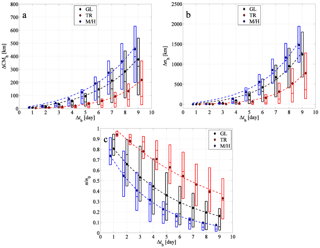
Figure 7.
(a) The horizontal difference between the center of mass of the BWCs and the FWC depending on the time period of the backward simulation; (b) the difference between the horizontal standard deviations of the BWCs and FWC; (c) the proportion of the particles returned back to the initial cuboid. The results are shown for the tropical region (TR, red), for mid- and high latitudes (M/H, blue) and for the globe (GL, black). Mean values (diamonds), medians and lower and upper quartiles (boxes with horizontal lines) are indicated. Dashed lines indicate exponential fits to the mean values; the exponents are given in Table 2.
A rapid growth can also be seen in the diagram. For at most three-day backward simulations, remains below 10–50 km, which implies generally a good agreement in the extension of the BWC and FWC considering that ranges between 33 and 5480 km with an average of about 1100 km. As in Figure 5, the increase of for small values can be approximated by an exponential function. Similar to the case study, the long-term behavior can be fitted by a large-exponent power-law function, but an exponential function also fits to the entire interval. Here, we only show the latter fit.
The mean values of in Figure 7c exhibit an exponential decay as in the case study. The decay of the function is the slowest for the tropical region. The slower decrease is in agreement with the fact that the usual wind field of the tropics differs from that of the mid- and high latitudes, where permanently generated and dissipated cyclones dominate. The weaker shearing in the wind field in the tropics and, thus, the weaker chaoticity of advection results in more particles being able return to the initial volume. For small for the tropics, negative deviation appears between the means and medians (mean minus median); while for large for the mid- and high latitudes, positive deviations are the rule. This implies that, although, in the tropics, most of the pollutant clouds are advected relatively accurately back to their initial position, occasionally, can be small. Analogously, for a long time backward simulation, the chance of a particle of a pollutant cloud initiated in the mid-latitudes to get back to its initial cuboid is usually very small (note the narrow extension of the blue boxes in Figure 7c for days); there exist, however, specific cases when can even reach 0.85 (five days) and 0.55 (nine days) (not shown in Figure 7c). These features and the large uncertainty in in the tropics might be explained by the fact that, on the one hand, pollutant clouds in the tropics can become mixed into the extratropics (see, e.g., Figure 1) and vice versa, and on the other hand, clouds dispersing even in their original region can be subject to more intense or weaker circulation than the typical one in that region.
Figure 8 gives an overview of the statistical parameters and . As in the case study, and seem to decrease approximately exponentially over . The property of simulations with excessively bad coincidence of FWC and BWC for the tropics for small (where the difference between the mean and median is positive) and ones with better agreement than the average for mid- and high latitudes for large (where the mean minus median difference is negative) appear also in Figure 8. The overlap of the BWC and FWC reduces below 50% after six days of backtracking for the tropics and after three days for mid- and high latitudes. For large , the , as well as the is small; however, there is a factor of about eight and six between the values of tropical and non-tropical values, respectively. Table 2 presents the Λ values of the fitted exponential functions to the mean data. It reveals that the time-dependence of the different statistical parameters can be described by similar Λ values.
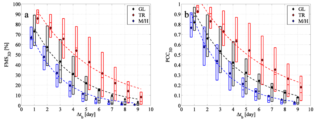
Figure 8.
(a) The figure of merit in space between the BWCs and FWC depending on the time period of the backward simulation; (b) Pearson’s correlation coefficient between the BWCs and FWC. Mean values (diamonds), medians and lower and upper quartiles (boxes with horizontal lines) are indicated for the tropical region (TR, red), for mid- and high latitudes (M/H, blue) and for the globe (GL, black). Dashed lines indicate exponential fits to the mean values; the exponents are given in Table 2.
7. Outlook
Although, in large-scale dispersion simulations, the effect of small-scale 3D turbulent diffusion on particles (taking effect below the grid-size of the meteorological data) can generally be neglected compared to that of advection, in order to obtain insight into how turbulent diffusion alters our findings, we repeated the simulation of the case study with a typical constant horizontal diffusivity of m·s [31]. Adding turbulent diffusion to the trajectory calculations can be considered as adding noise to the system. The effect of turbulent diffusion in the forward simulation over time t is enhanced further over an additional time interval of in the backward simulation. It broadens the extension of the pollutant cloud in backward mode, too, as also found in other dispersion models (see, e.g., [31]).
Table 3.
The exponent Λ (day) and the error of the exponential fits to the curves , , , , , and versus of the case study described in Section 5, but with horizontal turbulent diffusivity m·s. The deviation of the Λ values of the case study with turbulent diffusivity from the case study without turbulent diffusivity is also shown.
| - | Λ | |
|---|---|---|
Table 3 gives the exponents Λ of the curve fittings gained from the case study when adding turbulent diffusivity to the simulations. indicates the difference from the Λ values of Table 1. As expected, e.g., for , a somewhat faster decrease shows up, and the values are found 0.02–0.1 smaller at each than in the case without turbulent diffusion. Nevertheless, the change in Λ even for this quantity falls in the error bar of the fit. There are nearly no changes, neither in the data nor in Λ for , as turbulent diffusion has no direct impact on the center of mass. Only a slight increase is found for with about 30 km ( days) to about 100 km ( days) in the data. This is due to the fact that turbulent diffusion enhances the extension of both the forward and the backward cloud; however, in the latter case, diffusion acts on a time interval longer by . Nevertheless, neither does this significantly alter the value of Λ. It confirms the assumption that m·s has negligible effect on large-scale dispersion. The mean values of change about , while for , a definite decrease of 2%–10% appears for backward simulations of 1–5 days duration.
The results obtained in the presence of weak horizontal turbulent diffusion are practically the same as without any diffusion. This is consistent with the well-known property of low dimensional chaos according to which a weak noise washes out fine details below a characteristic length scale, but does not influence at all properties beyond that scale [16,40].
If the particles represent not passive tracers, rather aerosol particles with realistic radius r and density (e.g., m, kg·m), Equation (1) contains an additional term describing the gravitational settling of the particles [25]. In this case, particles can deposit on the ground in both the forward and the backward simulation, and during the backward one, particles that deposited in the forward run are treated as particles emitted from the surface in the appropriate time instant and location. This additional process shortens the time that the particles spend in the atmosphere before deposition (i.e., the time of the forward and backward tracking); nevertheless, our preliminary results show that the characteristics of the accuracy of backward tracking do not change.
8. Summary
In order to study the accuracy of backward trajectory simulations for locating the initial position of pollutant clouds precisely, we carried out, besides a case study, several simulations of pollutants distributed over the globe. Some characteristics of the backward and the forward pollutant clouds were determined at the same time instant. Forward pollutant clouds were considered as “real” clouds with which the results of the backward simulation are expected to coincide under full time-reversibility.
The results reveal that for –3 days of backward simulations, a reasonable agreement of the backward and forward clouds can be found, that is the backward tracking for such time periods performs reasonably well. This agreement can be seen in the figures of the simultaneous plots of the backward and forward clouds, and statistical parameters also support this observation. The difference between the center of mass/standard deviation of the two pollutant clouds grows exponentially with the time interval of the backward simulation at any initial location over the globe, which can be considered to be a consequence of the chaotic motion of the particles. The accuracy of backward simulations proves to decrease exponentially, too, by studying the proportion of the particles that are able to get back to their initial volume, the figure of merit in space or the Pearson’s correlation coefficient between the backward and forward cloud. A faster decrease characterizes the mid- and high latitudes compared to the tropical region. The above-mentioned observations are also valid for simulations that take into account the effect of turbulent diffusion, as well.
Note that the time interval over which the accuracy of time-reversibility is found to be reasonable is on the order of magnitude of the predictability time of atmospheric dispersion (the reciprocal of the Lyapunov exponent), and furthermore, this is on the same order as the predictability time of the wind field [41].
We conclude that aside from rare occasions with calm weather conditions and weak wind shear (especially in the tropics), with the resolution of the meteorological data used here, backward tracking of pollutant clouds is not reliable beyond a few days. On time scales longer than this, simulations may yield an error of about several 100 km in the position of the center of mass, and the overlap and Pearson’s correlation coefficient also fall below , usually considered as a limit of predictability.
Although results in the coincidence of the forward and backward clouds may be improved by applying more sophisticated numerical schemes and meteorological data with finer resolution at the expense of computational cost, it is not expected to basically alter the dynamics of the time-dependence of the quantities investigated, due to the unavoidable exponential degradation of the accuracy of dispersion simulations in our chaotic atmosphere.
Acknowledgments
The author thanks the useful discussions and suggestions of Tamás Tél, Gábor Drótos and Ulrike Feudel. Zoltán Rácz, Miklós Vincze and Tamás Weidinger are also acknowledged for valuable comments and remarks. This work was supported by the Hungarian Science Foundation under Grant OTKA NK100296.
Conflicts of Interest
The author declares no conflict of interest.
References
- Onishi, K.; Kurosaki, Y.; Otani, S.; Yoshida, A.; Sugimoto, N.; Kurozawa, Y. Atmospheric transport route determines components of Asian dust and health effects in Japan. Atmos. Environ. 2012, 49, 94–102. [Google Scholar] [CrossRef]
- Rao, K.S. Source estimation methods for atmospheric dispersion. Atmos. Environ. 2007, 41, 6964–6973. [Google Scholar]
- Seibert, P. Inverse modelling of sulfur emissions in Europe based on trajectories. In Inverse Methods in Global Biogeochemical Cycles; Kasibhatla, P., Heimann, M., Rayner, P., Mahowald, N., Prinn, R., Hartley, D., Eds.; American Geophysical Union: Washington, DC, USA, 2000; pp. 147–154. [Google Scholar]
- Uliasz, M.; Pielke, R.A. Application of the receptor oriented approach in mesoscale dispersion modeling. In Air Pollution Modeling and Its Application VIII; Springer: Berlin, Germany, 1991; pp. 399–407. [Google Scholar]
- Issartel, J.P.; Baverel, J. Inverse transport for the verification of the Comprehensive Nuclear Test Ban Treaty. Atmos. Chem. Phys. 2003, 3, 475–486. [Google Scholar] [CrossRef]
- Mori, I.; Nishikawa, M.; Quan, H.; Morita, M. Estimation of the concentration and chemical composition of kosa aerosols at their origin. Atmos. Environ. 2002, 36, 4569–4575. [Google Scholar] [CrossRef]
- Lin, T.H. Long-range transport of yellow sand to Taiwan in spring 2000: Observed evidence and simulation. Atmos. Environ. 2001, 35, 5873–5882. [Google Scholar] [CrossRef]
- Šauliene, I.; Veriankaite, L. Application of backward air mass trajectory analysis in evaluating airborne pollen dispersion. J. Environ. En. Landsc. Manag. 2006, 14, 113–120. [Google Scholar]
- Zemmer, F.; Karaca, F.; Ozkaragoz, F. Ragweed pollen observed in Turkey: Detection of sources using back trajectory models. Sci. Tot. Environ. 2012, 430, 101–108. [Google Scholar] [CrossRef] [PubMed]
- Drumond, A.; Nieto, R.; Gimeno, L.; Ambrizzi, T. A Lagrangian identification of major sources of moisture over Central Brazil and La Plata Basin. J. Geophys. Res. Atmos. 2008, 113, D14. [Google Scholar] [CrossRef]
- Straub, C.; Tschanz, B.; Hocke, K.; Kämpfer, N.; Smith, A. Transport of mesospheric H2O during and after the stratospheric sudden warming of January 2010: observation and simulation. Atmos. Chem. Phys. 2012, 12, 5413–5427. [Google Scholar] [CrossRef]
- Flesch, T.K.; Wilson, J.D.; Yee, E. Backward-time Lagrangian stochastic dispersion models and their application to estimate gaseous emissions. J. Appl. Meteorol. 1995, 34, 1320–1332. [Google Scholar] [CrossRef]
- Kljun, N.; Rotach, M.; Schmid, H. A three-dimensional backward Lagrangian footprint model for a wide range of boundary-layer stratifications. Bound. Layer Meteorol. 2002, 103, 205–226. [Google Scholar] [CrossRef]
- Dahl, J.M.; Parker, M.D.; Wicker, L.J. Uncertainties in trajectory calculations within near-surface mesocyclones of simulated supercells. Mon. Weather Rev. 2012, 140, 2959–2966. [Google Scholar] [CrossRef]
- Lorenz, E.N. Deterministic nonperiodic flow. J. Atmos. Sci. 1963, 20, 130–141. [Google Scholar] [CrossRef]
- Ott, E. Chaos in Dynamical Systems; Cambridge University Press: Cambridge, UK, 1993. [Google Scholar]
- Tél, T.; Gruiz, M. Chaotic Dynamics; Cambridge University Press: Cambridge, UK, 2006. [Google Scholar]
- Ottino, J. The Kinematics of Mixing: Stretching, Chaos, and Transport; Cambridge University Press: Cambridge, UK, 1989. [Google Scholar]
- Haszpra, T.; Tél, T. Topological entropy: A Lagrangian measure of the state of the free atmosphere. J. Atmos. Sci. 2013, 70, 4030–4040. [Google Scholar] [CrossRef]
- Pudykiewicz, J.A. Application of adjoint tracer transport equations for evaluating source parameters. Atmos. Environ. 1998, 32, 3039–3050. [Google Scholar] [CrossRef]
- Pierrehumbert, R.T.; Yang, H. Global chaotic mixing on isentropic surfaces. J. Atmos. Sci. 1993, 50, 2462–2480. [Google Scholar] [CrossRef]
- Shepelyansky, D.L. Some statistical properties of simple classically stochastic quantum systems. Physica D 1983, 8, 208–222. [Google Scholar] [CrossRef]
- Straume, A.G. A more extensive investigation of the use of ensemble forecasts for dispersion model evaluation. J. Appl. Meteorol. 2001, 40, 425–445. [Google Scholar] [CrossRef]
- Mosca, S.; Graziani, G.; Klug, W.; Bellasio, R.; Bianconi, R. A statistical methodology for the evaluation of long-range dispersion models: An application to the ETEX exercise. Atmos. Environ. 1998, 32, 4307–4324. [Google Scholar] [CrossRef]
- Haszpra, T.; Tél, T. Escape rate: A Lagrangian measure of particle deposition from the atmosphere. Nonlinear Process. Geophys. 2013, 20, 867–881. [Google Scholar] [CrossRef]
- Bowman, K.P.; Carrie, G.D. The mean-meridional transport circulation of the troposphere in an idealized GCM. J. Atmos. Sci. 2002, 59, 1502–1514. [Google Scholar] [CrossRef]
- Ryall, D.; Maryon, R. Validation of the UK Met. Office’s NAME model against the ETEX dataset. Atmos. Environ. 1998, 32, 4265–4276. [Google Scholar] [CrossRef]
- D’Amours, R.; Malo, A.; Ménard, S. A zeroth order Lagrangian particle dispersion model: MLDP0. Available online: http://eer.cmc.ec.gc.ca/publications/DAmours.Malo.2004.CMC-EER.MLDP0.pdf (accessed on 17 November 2015).
- Saltbones, J.; Foss, A.; Bartnicki, J. Norwegian Meteorological Institute’s real-time dispersion model SNAP (Severe Nuclear Accident Program): Runs for ETEX and ATMES II experiments with different meteorological input. Atmos. Environ. 1998, 32, 4277–4283. [Google Scholar] [CrossRef]
- Terada, H.; Chino, M. Development of an atmospheric dispersion model for accidental discharge of radionuclides with the function of simultaneous prediction for multiple domains and its evaluation by application to the Chernobyl nuclear accident. J. Nucl. Sci. Technol. 2008, 45, 920–931. [Google Scholar] [CrossRef]
- Stohl, A.; Forster, C.; Frank, A.; Seibert, P.; Wotawa, G. Technical note: The Lagrangian particle dispersion model FLEXPART version 6.2. Atmos. Chem. Phys. 2005, 5, 2461–2474. [Google Scholar] [CrossRef]
- Draxler, R.; Hess, G. NOAA Technical Memorandum ERL ARL-224. Description of the HYSPLIT_4 Modeling System; Air Resources Laboratory: Silber Spring, MD, USA, 2004. [Google Scholar]
- Dee, D.P.; Uppala, S.M.; Simmons, A.J.; Berrisford, P.; Poli, P.; Kobayashi, S.; Andrae, U.; Balmaseda, M.A.; Balsamo, G.; Bauer, P.; et al. The ERA-Interim Reanalysis: Configuration and performance of the data assimilation system. Q. J. R. Meteorol. Soc. 2011, 137, 553–597. [Google Scholar] [CrossRef]
- Stohl, A.; Wotawa, G.; Seibert, P.; Kromp-Kolb, H. Interpolation errors in wind fields as a function of spatial and temporal resolution and their impact on different types of kinematic trajectories. J. Appl. Meteorol. 1995, 34, 2149–2165. [Google Scholar] [CrossRef]
- Stohl, A.; Seibert, P.; Wotawa, G.; Arnold, D.; Burkhart, J.; Eckhardt, S.; Tapia, C.; Vargas, A.; Yasunari, T. Xenon-133 and caesium-137 releases into the atmosphere from the Fukushima Dai-ichi nuclear power plant: determination of the source term, atmospheric dispersion, and deposition. Atmos. Chem. Phys. 2012, 12, 2313–2343. [Google Scholar] [CrossRef]
- McCaw, G. Long lines on the Earth. Emp. Surv. Rev. 1932, 1, 259–263. [Google Scholar]
- Artale, V.; Boffetta, G.; Celani, A.; Cencini, M.; Vulpiani, A. Dispersion of passive tracers in closed basins: Beyond the diffusion coefficient. Phys. Fluids 1997, 9, 3162–3171. [Google Scholar] [CrossRef]
- Huber, M.; McWilliams, J.C.; Ghil, M. A climatology of turbulent dispersion in the troposphere. J. Atmos. Sci. 2001, 58, 2377–2394. [Google Scholar] [CrossRef]
- Von Hardenberg, J.; Fraedrich, K.; Lunkeit, F.; Provenzale, A. Transient chaotic mixing during a baroclinic life cycle. Chaos 2000, 10, 122–134. [Google Scholar] [CrossRef] [PubMed]
- Ben-Mizrachi, A.; Procaccia, I.; Grassberger, P. Characterization of experimental (noisy) strange attractors. Phys. Rev. A 1984, 29, 975–977. [Google Scholar] [CrossRef]
- Kalnay, E. Atmospheric Modeling, Data Assimilation, and Predictability; Cambridge University Press: Cambridge, UK, 2003. [Google Scholar]
© 2016 by the author; licensee MDPI, Basel, Switzerland. This article is an open access article distributed under the terms and conditions of the Creative Commons by Attribution (CC-BY) license (http://creativecommons.org/licenses/by/4.0/).