A Comparison of ETKF and Downscaling in a Regional Ensemble Prediction System

Abstract

Based on the operational regional ensemble prediction system (REPS) in China Meteorological Administration (CMA), this paper carried out comparison of two initial condition perturbation methods: an ensemble transform Kalman filter (ETKF) and a dynamical downscaling of global ensemble perturbations. One month consecutive tests are implemented to evaluate the performance of both methods in the operational REPS environment. The perturbation characteristics are analyzed and ensemble forecast verifications are conducted; furthermore, a TC case is investigated. The main conclusions are as follows: the ETKF perturbations contain more power at small scales while the ones derived from downscaling contain more power at large scales, and the relative difference of the two types of perturbations on scales become smaller with forecast lead time. The growth of downscaling perturbations is more remarkable, and the downscaling perturbations have larger magnitude than ETKF perturbations at all forecast lead times. However, the ETKF perturbation variance can represent the forecast error variance better than downscaling. Ensemble forecast verification shows slightly higher skill of downscaling ensemble over ETKF ensemble. A TC case study indicates that the overall performance of the two systems are quite similar despite the slightly smaller error of DOWN ensemble than ETKF ensemble at long range forecast lead times.

1. Introduction

It has long been known that numerical weather prediction (NWP) is sensitive to the initial condition (IC) error, model error and the chaotic nature of atmosphere, thus an ensemble prediction method [1] has emerged as a practical way for providing probabilistic forecasts. Since the ensemble predictions implemented operationally in the early 1990s at the National Centers for Environmental Prediction [2] and at the European Center for Medium-Range Weather Forecast [3], an ensemble prediction system (EPS) has been operational in many meteorological centers to provide operational global weather forecast [4,5,6].

Since the probability distribution for the various sources of errors are more complicated for regional NWP, it is difficult to predict the meso-scale severe weather. It seems that developing a regional ensemble prediction system (REPS) is a practical way to solve this problem. How to generate IC perturbations for regional ensemble prediction is an important issue. One of the possible choices is dynamical downscaling of a global EPS, which interpolates forecast fields from a set of representative members of the global EPS to obtain different ICs for the regional domain with higher resolution. This method has been successfully applied in some current operational REPS [7,8,9]. Recently, downscaled IC perturbations have also been successfully applied in experimental convection-permitting REPSs with higher resolution [10,11]. In these convection-permitting ensembles, an intermediate resolution REPS is typically used to transfer the information in a chain of forecasts from the coarse-resolution global EPS to the high-resolution REPS. Although dynamical downscaling is attractive for its simplicity and good performance, the regional small-scale uncertainties cannot be explicitly represented with dynamical downscaling but just following the governance of the global ensemble that is driving it [12]. Some other studies try to generate IC perturbations for REPS by using a regional version of traditional IC perturbation methods, such as the Breeding Growing Mode (BGM), Singular Vectors (SVs), Ensemble Transform Kalman Filter (ETKF), etc. It is proved that these methods can also trigger limited ensemble spread and benefit forecast skill for REPS [13,14,15,16].

However, so far it is still unclear whether these regional versions of IC perturbation methods, as primarily designed for medium-range forecasting, are fully superior to downscaling when applied to REPS. Bowler and Mylne [17] tested ETKF and downscaling as the IC perturbations generators for a regional version of MetOffice Global and Regional Ensemble Prediction System (MOGREPS), and revealed that the perturbations generated by regional ETKF contain more detail at small scales and less power at large scales with less than 18 h forecast lead time. These perturbations are overall smaller than the ones derived from the downscaling, and the skill of the two ensembles is very similar, with slightly higher skill being seen from the downscaling. Whereas the comparison results of downscaling and regional IC perturbation generators presented by Saito et al. [18] are mixed, as the downscaling method tends to perturb synoptic-scale disturbances and showed the best ratio of the ensemble spread to the RMSE, while the regional version of BGM, ET and SVs tend to perturb meso-scale disturbances, thus affecting local intense rains more. Although whether these regional IC perturbation generators can yield advantage over dynamical downscaling is still obscure, there is no doubt that these methods can produce more information of small/meso-scale uncertainties than dynamical downscaling, and this information is particularly useful for the forecasting of local severe convective weather [19,20].

The CMA has been operationally running a REPS since May, 2014, with the IC perturbations generated by a regional version of ETKF. Since this operational REPS is coupled with an operational global ensemble prediction system (GEPS) of CMA, it is also possible for the REPS to obtain IC perturbation from dynamical downscaling of global ensemble perturbations. This paper will give a detailed comparison of ETKF and downscaling in the operational REPS environment. In the study we hope to have a further understanding of the advantages and disadvantages of the two typical kinds of IC perturbation methods, and this investigation is also expected to provide some information for the improvement of the present REPS in the future.

The outline of this article is as follows. Section 2 describes the ensemble forecasting system, the structure of the IC perturbations, and the investigation set-up. Section 3 presents the results and discussion from the evaluation of perturbation quality and various ensemble forecast quality measures. Afterwards, the Typhoon track forecast quality is investigated. A summary and conclusions of the obtained results is provided in Section 4.

2. System and Method

2.1. Introduction of the Regional Ensemble Prediction System

The REPS in CMA has been running operationally so far, this system with relatively high-resolution aims at providing probabilistic forecast for meso/small-scale severe weather phenomenon, such as heavy precipitation and tropical cyclone (TC).

This REPS is constructed based on a regional model of GRAPES-Meso (regional version of Global and Regional Assimilation and Prediction System) [21]. The GRAPES-Meso regional model runs on a regular latitude-longitude grid with a resolution of 0.15 degree in the horizontal and 33 model levels vertically. Model domain is set to 70–145.15°E, 15–64.35°N, covering the whole area of China. The IC perturbations of this REPS (abbreviated as GRAPES-REPS) are generated by a regional ETKF approach, and the model uncertainty is represented by multiple physics [4]. Since the GRAPES-REPS have coupled with the GEPS of CMA, the lateral boundary conditions (LBCs) of the GRAPES-REPS are also perturbed. Figure 1 shows the model domain of GRAPES-REPS that nested in the global ensemble. The GRAPES-REPS consist of 15 members, including a control run and 14 perturbed ensemble members. In each day the system started at 0600 UTC, 1200 UTC, 1800 UTC and 0000 UTC. For each start time the system provide 6 h forecast perturbations for the next ETKF cycle, specifically for 1200 UTC and 0000 UTC initiate time the model integrate to 72 h to provide ensemble forecast products. Five variables (zonal wind u, meridional wind v, potential temperature θ, Exner pressure π and specific humidity q) in the ICs are perturbed.

Figure 1. Model domain of GRAPES-REPS within a global ensemble.

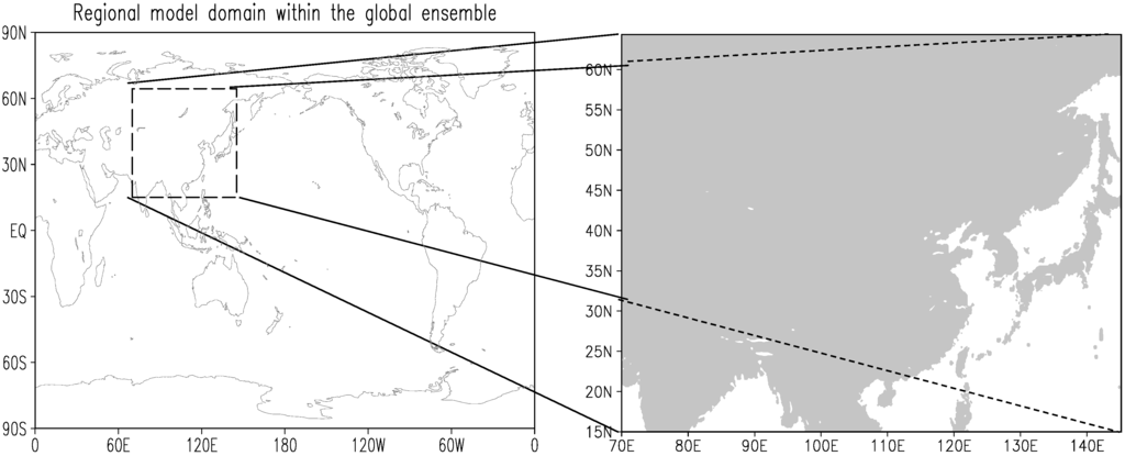
Figure 1. Model domain of GRAPES-REPS within a global ensemble.

2.2. Introduction of the IC Perturbation Schemes

In our study, two IC perturbation schemes are used, one is regional ETKF (as applied in the operational run), and the other is dynamical downscaling of the GEPS.

2.2.1. ETKF

Wang and Bishop [22] demonstrated the viability and effectiveness of ETKF in generating IC perturbations (as also called analyses perturbations) for global ensemble forecast. The ETKF can generate IC perturbations that correspond well to the observational density. In addition, compared with BGM technique that maintain variance in few directions, ETKF can maintain comparable amounts of variance in all orthogonal and uncorrelated directions spanning its ensemble perturbation subspace; moreover, the computation cost of ETKF is not much more than BGM.

The derivation of ETKF analyses perturbations is based on the hypothesis that the forecast covariance matrices and analysis covariance matrices can be represented by forecast perturbations X^f and analysis perturbations X^a. The relationship between X^f and X^a is established after solving the optimal data assimilation equation; as a result, the forecast perturbation can be transformed to analysis perturbation through a transformation matrix T, that is

$$X^a=X^{f}T\mathrm{\Pi }$$

(1)

where forecast perturbations are listed as columns in the matrix X^f and analysis perturbations are listed as columns in the matrix X^a. Π is a scalar inflation factor to inflate the analysis perturbation amplitude so as to ensure that the 6 h forecast ensemble variance is consistent with the control forecast error variance. Following Wang and Bishop, T is given by

$$T=C{(\mathrm{\Gamma }+I)}^{-1/2}{C}^T$$

(2)

where columns of the matrix C and Γ contain the eigenvectors and the corresponding eigenvalues of the matrix:

$${(Z^f)}^T{H}^T{R}^{-1}H{Z}^f$$

(3)

where the matrix H is the linear observation operator that maps model variables to observed variables and the matrix R is the observation error covariance matrix.

2.2.2. Dynamical Downscaling

A traditional “downscaling” mechanism is a process that aims at finding a mathematical relation between the global and local fields, that is stable in time and, valid for a variety of different meteorological systems. The generation of some systems (e.g., convective phenomenon) are too complicated to be linearly predictable from the large-scale flow, so the downscaling usually achieved by a complicated, nonlinear “transfer function” [23]. There are a variety of downscaling techniques in the literature, but two major approaches can be identified at the moment, namely, dynamical downscaling and empirical (statistical) downscaling. Dynamical downscaling approach is a method of extracting local-scale information by regional models with the coarse global data used as boundary conditions [24]. For a regional ensemble forecast, the dynamical downscaling of an ensemble of global IC stats will produce the IC stats of regional ensemble [25]. Generally, this downscaling approach to generate IC perturbations for REPS is attractive due to its relative simplicity and practicality of implementation.

The resolution of the GEPS in CMA is T639L60 (spectral triangular T639 with 60 vertical levels, corresponding to 30 km resolution). A masked breeding method [26] is applied to compute ICs of this GEPS, with 12 h optimization time interval. For each initial time, the forecast perturbations of the pervious breeding cycle are scaled to have initial amplitude comparable to an estimate of the analysis error. Mathematically,

$$X_{ij}^a=X_{ij}^f{c}_{ij}$$

(4)

where X^a_ij and X^f_ij are analysis perturbations and forecast perturbations at latitude i and longitude j, c_ij is a rescaling factor which is a function of latitude and longitude.

The background state as well as the LBCs of GRAPES-REPS is provided by a GEPS. This configuration enable IC perturbations of GRAPES-REPS be obtained from dynamical downscaling of this GEPS. This is achieved by interpolating the IC stats of GEPS to the 0.15 by 0.15 degree resolution through the initialization process of GRAPES-Meso regional model.

2.3. Experimental Set-Up

In the present study, the ETKF method and the downscaling method are compared using the same unperturbed analysis and the same forecast model. The numerical experiments are based on the operational GRAPES-REPS of CMA. The regional ensemble was run twice to produce forecasts, one set of forecasts generated IC perturbations by the regional ETKF, and the other was run using a downscaling of the global perturbations as IC perturbations.

The two different ensembles compared in this work will be denoted as ETKF and DOWN. The one-month period of 1 August 2012 to 31 August 2012 is chosen to conduct this comparison test, with both sets of ensembles initiated at 1200 UTC each day. Forecasts were evaluated to a lead-time of 72 h. The system settings of the two tests are identical to the operational run.

The background state and the LBCs of experimental REPS are provided by T639 global ensemble forecast data. The T639 global analysis states corresponding to each forecast lead times of the forecasts are interpolated to a common regular 0.15 by 0.15 degree resolution to verify the forecasts of upper air weather variables. The observational TC track data are provided by the Joint Typhoon Warning Center (JTWC) Best Track.

3. Results and Discussion

We now evaluate the quality of IC perturbation states and ensemble forecasts from each methodology. For a regional ensemble forecast, it is desirable to provide information of all scales, not only synoptic scales but also convective scales, therefore we start with an examination of the scale characteristics of ETKF perturbations and DOWN perturbations. Next, since the ensemble spread growth is closely correlated with the perturbation growth, we investigate how the two types of perturbations evolve, and how the perturbation amplitude increase with lead time. In addition, an “ensemble perturbation precision test” is conducted to determine whether the two perturbation techniques can better represent the forecast errors (e.g., locations where perturbation amplitude is large corresponds to locations where forecast error is large). Thereafter, we statistically evaluate the ensemble forecast skill, with a series of probability verification scores used. We will also present a study to evaluate the practicability of two methods in a particular weather case.

3.1. Power Spectra Analysis

A good ensemble forecast can provide sufficient uncertainty information, either for small-scale phenomenon or for large-scale phenomenon. The spatial scale characteristics of two types of perturbations are investigated, this is achieved by calculating the power spectra of both the ETKF and DOWN perturbations. A 2-dimemsional Discrete Cosine Transform (2D-DCT) [27], which is suitable for spectral analysis of data on a limited area, is used to conduct power spectra analyses. We first find the difference between each perturbed forecast and the ensemble mean, and then calculate the power spectra by 2D-DCT. The power spectra are calculated for each ensemble member, to create an average power spectra value.

Figure 2 shows power spectra of 500 hPa temperature perturbations as a function of wavelength, for both ETKF perturbations and DOWN perturbations. The power spectra of initial perturbations and 6 h forecast perturbations are presented. Results from initial (00 h) forecasts (Figure 2a) show that the power of the ETKF perturbations is greater than that of the downscaling perturbations at wavelengths less than 1100 km. In particular, for wavelengths less than 60 km (around two grid lengths of the T639 global model), there is no power for the global ensemble perturbations. These scales cannot be better resolved by the global model, so the perturbations derived from the global ensemble exhibit less power at these length-scales. Whereas for scales over 1100 km more power can be found in DOWN ensemble, as the maximum power can reach to 40 k² (corresponding to wavelength of 5000 km), while the maximum value for ETKF ensemble can only reach to 20 k² (corresponding to wavelength of 3200 km). The results from 12 h forecasts (Figure 2b) show that the scale characteristics of the two perturbation schemes get closer with forecast lead time. The 12 h ETKF perturbations exhibit amplified power than that of 00 h at larger scales, and the most powerful scale is 5000 km, with the power value of 60 K²; while the 12 h downscaling perturbations have increased power than that of 00 h at all length-scales, including the small-scales that cannot be resolved by downscaling perturbations at initial time.

Figure 2. All member averaged power spectra of 500 hPa temperature perturbations as a function of wavelength for ETKF and DOWN. (a) Initial time; (b) 12 h forecast lead time.

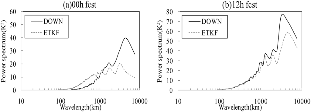
Figure 2. All member averaged power spectra of 500 hPa temperature perturbations as a function of wavelength for ETKF and DOWN. (a) Initial time; (b) 12 h forecast lead time.

The results presented above indicate, when applied to the self cycling of GRAPES-REPS, the ETKF technique can create analysis perturbations from forecast perturbations which are completely produced by regional model and hence, in principle, provide IC perturbations at all scales resolved by regional model. The greater power of small-scales can enable the ETKF perturbations to better capture the convective, high impact weather uncertainty, whereas the downscaling perturbations could not represent the small-scale uncertainty at the initial time, and are better than ETKF at representing the large-scale uncertainty.

3.2. Perturbation Growth Characteristics

It has just been shown that the ETKF perturbations have greater power at smaller scales while the DOWN perturbations have greater power at larger scales. In order to investigate the perturbation characteristic intuitively, an attempt has been made to account for the distribution and evolution characteristics of both kinds of perturbations. This is achieved by calculating an “approximate energy norm” [28], defined as

$$\frac{1}{2}\left[{u^{\prime }}^2(i,j,k)+{v^{\prime }}^2(i,j,k)\right]+\frac{c_p}{T_r}{T^{\prime }}^2(i,j,k)$$

(5)

where uʹ, vʹ and Tʹ are wind and temperature perturbations, c_p is the specific heat and T_r is the reference temperature.

Figure 3 shows horizontal distributions of the energy norm averaged over all members at all levels, for both ETKF (left panel) and downscaling (right panel) ensembles, respectively. For the ETKF ensemble, the energy norm of analysis perturbations (Figure 3a) in eastern China is generally lower than that in the plateau and Western Pacific regions, due to the larger number of observations in this region. For the downscaling ensemble, the energy norm of analysis perturbations (Figure 3b) distribution do not show obvious observation impact because the rescaling factors in the global masked breeding are designed empirically from climatology data, although the global observation distribution in the mask is considered, the breed perturbations cannot reflect the regional observations distribution in detail. Additionally, the ETKF analysis perturbations exhibit more small-scale characteristic than DOWN analysis perturbations, while the DOWN perturbation pattern is larger in scale, and this difference can also reflect the analysis result in Section 3.1.

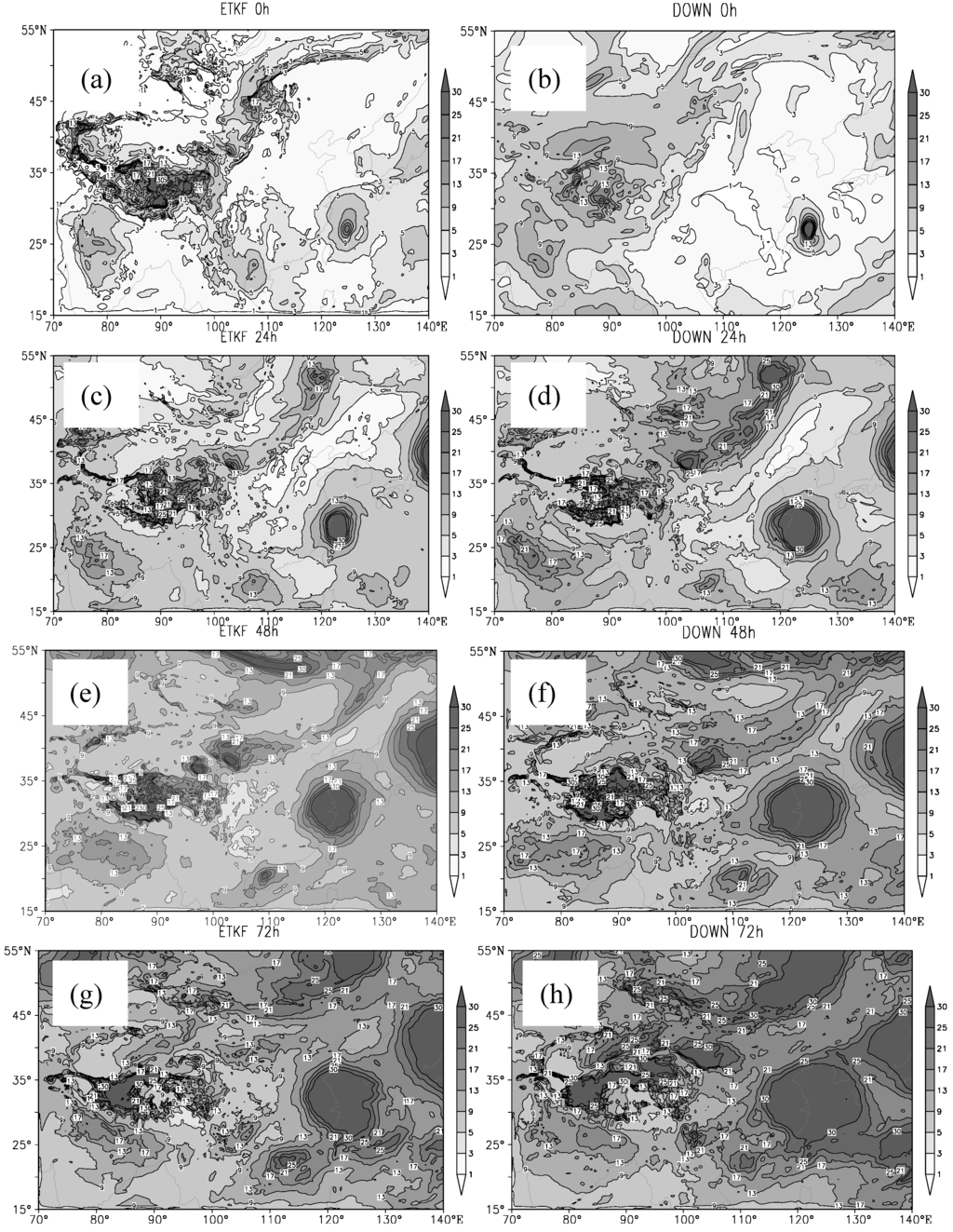
Figure 3. All members vertically averaged perturbation energy norm (unit:J/kg) at different forecast lead times, for ETKF and DOWN, respectively. (a) ETKF 00 h; (b) DOWN 00 h; (c) ETKF 24 h; (d) DOWN 24 h; (e) ETKF 48 h; (f) DOWN 48 h; (g) ETKF 72 h; and (h) DOWN 72 h.

Figure 3. All members vertically averaged perturbation energy norm (unit:J/kg) at different forecast lead times, for ETKF and DOWN, respectively. (a) ETKF 00 h; (b) DOWN 00 h; (c) ETKF 24 h; (d) DOWN 24 h; (e) ETKF 48 h; (f) DOWN 48 h; (g) ETKF 72 h; and (h) DOWN 72 h.

For 24 h forecast lead time (Figure 3c,d), the perturbations for both ensembles show remarkable growth, especially for DOWN perturbations in Western Pacific regions. With the increase of forecast lead time, the perturbation patterns for both ensembles become similar. Take 48 h (Figure 3e,f) and 72 h (Figure 3g,h) forecast lead times for example, the large perturbations regions in both ETKF and DOWN perturbation states correspond very well. The results indicate that the difference between the two systems in the perturbation distribution pattern for short range forecast is more significant than that of long range forecast.

Aside from the perturbation distribution pattern, it is desirable to compare both ensembles in terms of perturbation magnitude. We average the perturbation energy norm at all grid points at each level to get the vertical distributions of energy norm. Figure 4 illustrates such energy norm profiles for 0–36 h forecast lead times. The energy norm of ETKF ensemble (Figure 4a) can keep steady growth with forecast lead time, and the most remarkable growth level is around 250 hPa. For example, at 6 h lead time, the energy norm at 250 hPa is 2.7 J/kg, while at 36 h lead time, the corresponding value is 4 J/kg. The energy value at higher or lower levels is relatively smaller. For DOWN ensemble, the energy norm growth characteristics are similar. The largest energy norm can also be found at 250 hPa, with a value of 3.4 J/kg for 6 h forecast lead time and it 4.4 J/kg for 36 h lead time. It should be noted that the energy norm of DOWN ensemble perturbations is always larger than that of the ETKF ensemble perturbations at corresponding levels and corresponding lead times.

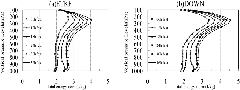
Figure 4. Vertical distributions of ensemble mean total energy (unit: J/kg), different lines denote different forecast lead times. (a) ETKF; (b) DOWN.

Figure 4. Vertical distributions of ensemble mean total energy (unit: J/kg), different lines denote different forecast lead times. (a) ETKF; (b) DOWN.

3.3. Ensemble Perturbation Precision Test

While larger perturbation values can indicate the larger magnitude of spread (as larger spread is always desirable for ensemble forecast), it is also interesting and important to investigate the “ensemble perturbation precision”. Studies by Toth et al. [29] and Zhu et al. [30] suggest that the ability of an ensemble to predict case-dependent forecast uncertainty is a critical criterion to evaluate an ensemble forecast system. The true forecast error variance can be regarded as a random variable around the ensemble perturbation variance. An accurate prediction of forecast error variance is one in which the true forecast error variance distributes closely to the ensemble perturbation variance; that is, the difference of the forecast error variance around the ensemble perturbation variance is small. We refer to the ability of an ensemble to get forecast error variance right on every day at every grid point variable as “the precision” of the ensemble perturbation variance [22]. Information about the degree of ensemble variance precision can be used to increase the accuracy of error probability density functions derived from ensemble variances. Here, we introduce tests of ensemble variance precision.

To analyze how well the ensemble perturbation variance can explain the forecast error variance, we follow the method used by Wang and Bishop [22] and Wei et al. [6]. First, we compute the ensemble perturbation variance and squared error of a variable at each grid point of a particular pressure level. A scatterplot (which is not shown) can then be drawn by using ensemble perturbation variance (abscissa) and forecast errors variance for all grid points. Since the grid points for the both REPSs are 502 × 330, we next divide the points into 330 equally populated bins (with 502 grid points in each bin) in order of increasing ensemble variance. The ensemble and forecast variances are then averaged within each bin. It is the averaged values from each bin that are plotted. The relationship between ensemble perturbation variance and forecast error variance of 500 hPa temperature for ETKF and DOWN ensembles in forms of such plot are shown in Figure 5. If the number of bins is reduced (e.g., 33 bins with 5020 grid points in each bin), it is expected that the curve will be smoother. The result from 33 bins is shown by a solid line. For 6 h forecast (Figure 5a,b), the results from the 330-bin case (dotted line) show that the range of forecast error variance (maximum minus minimum values) explained by the ensemble variance is larger for ETKF(3.3 K²) than DOWN (0.4 K²). For 33-bin case (solid line), the range of forecast error variance explained by ETKF ensemble variance is also larger (1.5 K²) than that of DOWN (0.3 K²). This shows that ETKF perturbations are better than DOWN perturbations at being able to distinguish times and locations where forecast errors are likely to be large from the times and locations where forecast errors are likely to be small. For 60 h lead time (Figure 5c,d), the range of forecast error variance (10.8 K² from 330-bin case and 8.3 K² from 33-bin case) explained by ETKF ensemble variance is still larger than that of DOWN ensemble (9.5 K² from 330-bin case and 7.5 K² from 33-bin case), but the difference between the two ensembles become smaller, compared to the 6 h forecast.

Figure 5. Relationship between the 500 hPa temperature ensemble perturbation variance and forecast error variances with the value averaged from each of 33 bins (solid lines) and 330 bins (dotted lines) at all grid points. (a) ETKF 6 h forecast; (b) DOWN 6 h forecast; (c) ETKF 60 h forecast; (d) DOWN 60 h forecast.

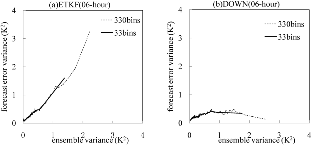
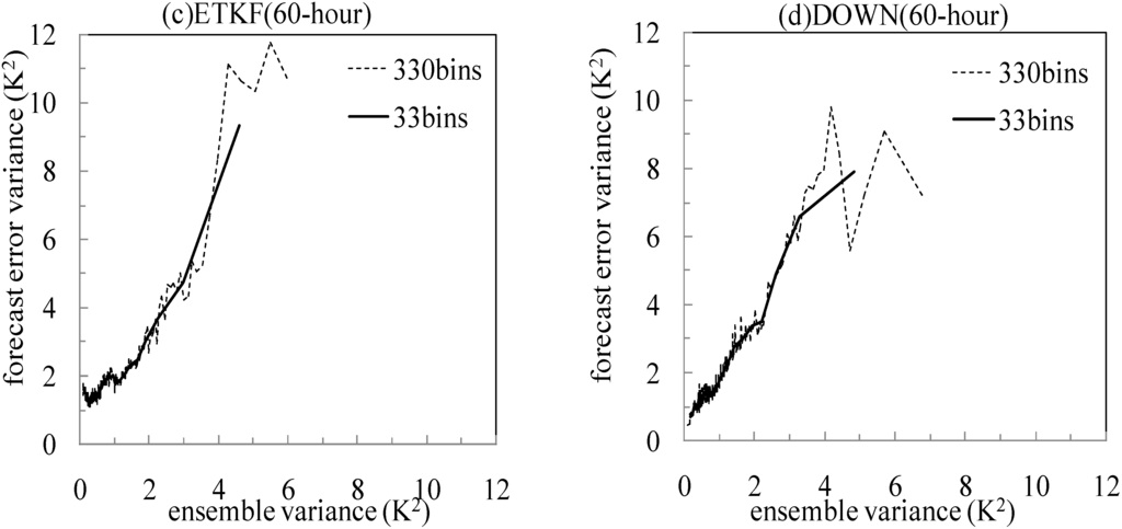
Figure 5. Relationship between the 500 hPa temperature ensemble perturbation variance and forecast error variances with the value averaged from each of 33 bins (solid lines) and 330 bins (dotted lines) at all grid points. (a) ETKF 6 h forecast; (b) DOWN 6 h forecast; (c) ETKF 60 h forecast; (d) DOWN 60 h forecast.

3.4. Ensemble Verification Results

To compare the results of both perturbation methods, we have used several verification methods. The methods are root mean square error (RMSE) for ensemble mean, the ensemble spread, the continuous ranked probability skill score (CRPS), and the Talagrand diagram. The results are reported for several model output variables.

3.4.1. Root Mean Square Error and Ensemble Spread

A useful measure of the skill of an ensemble prediction system is how well the variation in the spread (deviation of the ensemble about its mean) of the ensemble matches the variation in the RMSE of the ensemble mean forecast. We calculated the spatially averaged spread of all variables at all levels for each lead time, and compared this to a spatially averaged RMES of the ensemble mean. Figure 6 shows one-month averaged ensemble mean RMSE and ensemble spread for ETKF ensemble and DOWN ensemble, with two upper air variables of 500 hPa wind speed (WS500), 850 hPa temperature (T850) and one near surface variable of 10 m U wind (U10m) presented for comparison. It turns out that for all these variables, both methods have a lack of spread, and spread growth is slower than RMSE growth for both ensembles. Overall, the DOWN ensemble shows larger spread at all forecast lead times comparatively, with relatively smaller RMSE. Similar results can also be observed for other variables at different pressure levels (not shown). The results suggest that the larger spread of DOWN ensemble can really enhance the accuracy of ensemble mean forecast.

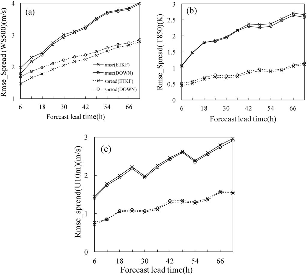
Figure 6. RMSE of ensemble mean and ensemble spread for ETKF and DOWN, respectively. (a) 500 hPa wind speed; (b) 850 hPa temperature; (c) 10 m U wind.

Figure 6. RMSE of ensemble mean and ensemble spread for ETKF and DOWN, respectively. (a) 500 hPa wind speed; (b) 850 hPa temperature; (c) 10 m U wind.

3.4.2. Continuous Rank Probability Score

The continuous rank probability score (CRPS) is an overall measure of the skill of a probabilistic prediction, measuring the skill of the ensemble mean forecast as well as the ability of the perturbations to capture the deviations around that. For a variable x, if the ensemble predicted probability density function is p(x) and the observational value is x_o, the CRPS is given by [31]

$$CRPS={{\displaystyle {\int }_{-\infty }^{\infty }\left[P(x)-H(x-x_o)\right]}}^{2}dx$$

(6)

where

$$P(x)={\displaystyle {\int }_{-\infty }^{x}p(y)dy}$$

(7)

and H(x) is the step function with:

$$H(x)=\{\begin{array}{l}0(x<0)\\ 1(x>=0)\end{array}$$

(8)

The CRPS is a penalty score, so smaller values are better. Figure 7 shows the CRPS of WS500, T850 and WS850 for both ETKF ensemble and DOWN ensemble. It is clear that the DOWN ensemble performs better (with smaller CRPS value) than ETKF for all the variables within 72 h lead times. CRPS verification on other variables can give similar results (not shown). This demonstrates that the DOWN method is better at providing probabilistic forecast than ETKF. Note, however, that the advantage of DOWN ensemble is quite limited, and the overall performances of the two ensembles are quite similar.

Figure 7. CRPS as a function of forecast lead time, for ETKF and DOWN, respectively. (a) 500 hPa wind speed; (b) 850 hPa temperature; (c)10 m U wind.

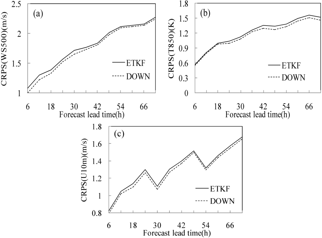
Figure 7. CRPS as a function of forecast lead time, for ETKF and DOWN, respectively. (a) 500 hPa wind speed; (b) 850 hPa temperature; (c)10 m U wind.

3.4.3. Talagrand Diagram

Another measure of statistical reliability is the Talagrand diagram [32]. This is the statistic of the frequency that the observation lays inside or outside the whole ensemble. A more reliable EPS should have a more flat pattern. “U” shape means lack of spread, “J” or “L” shapes mean there is bias in the system. Figure 8 shows the Talagrand diagram for WS500, T850 and U10m for 24 h lead time. It is evident that for all the graphs, the diagram of DOWN ensemble is closer to flat than the ETKF ensemble; this indicate that the frequency that observations lay inside the whole ensemble is higher for DOWN than ETKF. From Figure 6 we know that both ensembles are under-spread, thus, comparatively speaking, this more flat pattern of DOWN ensemble is desirable.

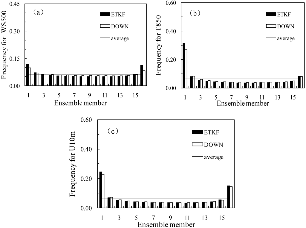
Figure 8. Talagrand for ETKF and DOWN at forecast lead time of 24 h. (a) 500 hPa wind speed; (b) 850 hPa temperature; (c)10 m U wind.

Figure 8. Talagrand for ETKF and DOWN at forecast lead time of 24 h. (a) 500 hPa wind speed; (b) 850 hPa temperature; (c)10 m U wind.

3.5. A TC Case Study

A TC case is studied to assess the practical performances of both ensembles. The 11th typhoon “Haikui” (1211) in 2012 was one of the most severe threats to Mainland China and caused several hazardous disasters, including heavy precipitation, windstorms, and storm surges. Haikui was born in the Central Pacific (about 140.7°E, 23.2°N) at 08030000 UTC and landed on Xiangshan in Zhejiang Province, China at 08071920 UTC (Figure 9). Graded as “severe typhoon” according to the CMA, Haikui was characterized by generation in the high latitude area, rapid intensification just before landing, and stagnation after landing. Here the track forecasts of Haikui (1211) within 72 h lead time from ETKF ensemble and DOWN ensemble are compared.

The predicted tracks of Haikui from ensemble members and ensemble mean of ETKF ensemble and DOWN ensemble are displayed in Figure 10. All forecasts are initiated at 08061200 UTC with a forecast length of 72 h. From the ETKF ensemble forecast (Figure 10a), we note that the tracks forecasted by all the members exhibit a divergence characteristic; this can reflect the spread growth with forecast lead time. The forecasted tracks from several ensemble members are very close to the observation, except the ones with drastic northward turning. From DOWN ensemble forecast (Figure 10b), it is clear that there are also some members that correspond well to the observation, and it seems that the ensemble mean forecast of DOWN is better than that of ETKF. A significant contrast of ETKF ensemble and DOWN ensemble is the variability of the directions between the forecasted tracks, since all the tracks forecasted by ETKF ensemble can pass through the rectangular region, while the tracks forecasted by DOWN ensemble are more diverged with some tracks laying outside of the rectangular region. Although this more dispersive distribution of DOWN forecasted tracks may possible to comprise the true TC course, such great spread of tracks might not be considered desirable as it can also brought confusing for users.

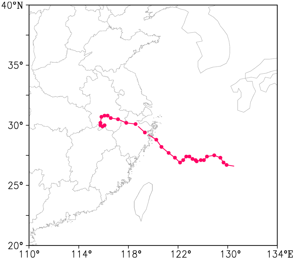
Figure 9. Observed Track of Haikui (1211).

Figure 9. Observed Track of Haikui (1211).

Figure 10. Seventy-two hour track forecasts of Haikui (1211) from ensemble forecasts of (a) ETKF and (b) DOWN. Red line is ensemble mean forecast (MEAN) and blue lines are ensemble member forecasts (EPS).

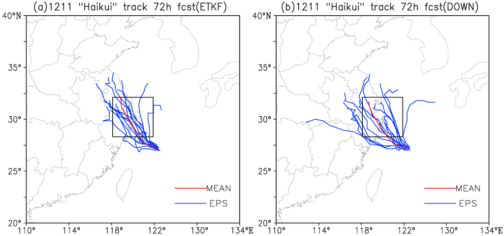
Figure 10. Seventy-two hour track forecasts of Haikui (1211) from ensemble forecasts of (a) ETKF and (b) DOWN. Red line is ensemble mean forecast (MEAN) and blue lines are ensemble member forecasts (EPS).

An objective of ensemble forecast is to improve the forecast accuracy. To assess the TC track forecast accuracy of the two ensembles, the track forecast error is studied. At one forecast lead time, the TC track forecast error is defined to be the distance of the forecasted track location from the observational location. Such forecast error in terms of track distance is displayed in Figure 11. As shown in Figure 11a, the 36 h forecast error of all ensemble members are limited within a range of 300 km, and the error of ensemble mean is 73 km at 36 h lead time, which is significantly less than most member forecasts. However, we can also find a significant error growth beyond 36 h lead time, and some members exhibit extremely large error, for example, there are three members whose error values are over 600 km at 72 h lead time. The 72 h forecast error of ensemble mean can still maintain a reasonable value of 387 km. As shown in Figure 11b, the error characteristic of DOWN ensemble is very similar to that of ETKF ensemble within 36 h forecast lead time, and the error of ensemble mean is small (66 km for 36 h forecast). After 36 h forecast, it is obvious that the error value of DOWN ensemble member forecasts cover a wider range than ETKF ensemble. The 72 h forecast error value of some members can reach 1160 km, while some members can exhibit very small errors (smaller than 50 km). The error value of ensemble mean is 363 km, which is a little less than that of ETKF.

Figure 11. Distance of forecasted tracks and the observational track of Haikui (1211) as a function of forecast lead time, for (a) ensemble members and ensemble mean of ETKF and (b) ensemble members and ensemble mean of DOWN, respectively.

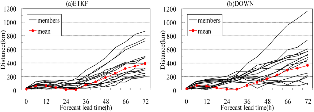
Figure 11. Distance of forecasted tracks and the observational track of Haikui (1211) as a function of forecast lead time, for (a) ensemble members and ensemble mean of ETKF and (b) ensemble members and ensemble mean of DOWN, respectively.

Generally speaking, the overall skills of the ensemble mean forecast of the two ensembles are very similar, and the DOWN ensemble has slightly higher skill for long forecast lead times. From this TC case study, it has not been possible to see clearly improved performance from either ensemble.

4. Summary and Conclusions

Based on the operational GRAPES-REPS, this paper carried out comparative studies on two IC perturbation schemes for regional ensemble, namely regional ETKF and dynamical downscaling. Using the two IC perturbation schemes, two consecutive ensemble forecast tests in an operational environment are conducted for a period of one month. The perturbation characteristics are investigated, meanwhile ensemble verification are implemented by use of several probability forecast verification methods. Additionally, a TC case of “Haikui” is studied to examine the practical effectiveness of the two regional ensemble forecasts. The main conclusions of this research are as follows:

The perturbations generated by ETKF have larger power at smaller scales, while the perturbations have more power at larger scales. The small-scale cannot be well resolved by the global model, so it is not surprising that the downscaling perturbations have a lack of small-scale power within short forecast range. With the forecast lead time increasing, the differences between ETKF and downscaling perturbations at different scales decrease.

The distribution pattern of both types of perturbations are quite different at initial time, the ETKF perturbations can reflect observation density while the downscaling distribution cannot. The two types of perturbations showed different growth characteristics, this is mainly due to the different ways in which the perturbations are calculated. The perturbations of the global ensemble are generated using a masked BGM, and the global perturbations at 12 h forecast lead time are rescaled by a rescaling factor, so that the perturbations can match approximately the global model forecast error at 12 h forecast lead time in the next cycle. When this is used to drive the IC perturbations for the regional model, the difference between the perturbed forecasts and the control forecast at initial time is relatively larger. When perturbations are calculated using the regional ETKF, the 6 h forecast perturbations are transformed and rescaled, and the perturbation magnitude will match the regional model forecast error at 6 h forecast lead time in the next ETKF cycle. Since there is significant difference between the calculated regional model 6 h forecast error and global model 12 h forecast error, the perturbation magnitude of the ETKF ensemble can be much less than that of the corresponding downscaling ensemble.

Although the downscaling perturbations shows better growth, these perturbations show no more skill than ETKF perturbations on representing forecast error. The range of forecast error variance explained by the ensemble variance is larger for ETKF than downscaling. This result indicate that the ETKF perturbations are better than downscaling perturbations at being able to distinguish times and locations where forecast errors are likely to be large from the times and locations where forecast errors are likely to be small.

The one-month statistics of ensemble verifications are also indicative. The RMSE and spread from the two ensembles show that the DOWN ensemble has slightly higher skill than the ETKF ensemble, and the results from CPRS and Talagrand histogram also support this conclusion. It is known that these scores can be influenced by the magnitude of the initial spread [5]. As Section 3.2 shows, the initial spread of DOWN ensemble is generally larger. This may reduce the forecast error of the DOWN ensemble. A conclusion will be drawn from the future comparison with both systems having similar initial spread.

A TC case study shows that the difference in the ensemble spread between the two systems dominate much of the comparison, the tracks from ETKF ensemble forecast are more concentrated, while the tracks from DOWN ensemble forecast are more dispersive. The track forecast error is also compared to assess whether there is any potential benefit from either system. It seem that the overall skill of the two systems are quite similar despite slightly smaller error of DOWN ensemble than ETKF ensemble at long range forecast lead times.

Now that a comprehensive comparison between IC perturbation methods of regional ETKF and dynamical downscaling has been made, one may revisit the question of whether it was right to implement this downscaling in the operational REPS of CMA, or if there is another way to improve the present ETKF based REPS. The results presented here indicate that the performance of the downscaling perturbations ensemble is better than that of the regional ETKF perturbations ensemble in some respects, such as the larger spread growth and better ensemble verification scores. Moreover, as described in Bowler and Mylne [15], the perturbations derived from downscaling are more consistent with the lateral boundary. However, there is no doubt that the downscaling perturbations have a lack of small-scale information, and the ETKF ensemble perturbations can better represent the forecast error of regional model. Although the above results are mixed, these comparisons may shed some light on further improvement in present system. A practical way to take advantages of both ensemble perturbations is developing a blending technique, which has been primarily investigated by Caron [33] and Wang et al. [34]. This technique can obtain blended perturbations that contain large-scale component from downscaling perturbations and small-scale component from ETKF perturbations. As this blending technique can take the advantages of both downscaling perturbations and regional ETKF perturbations, it is expected to be an appropriate way to achieving good ensemble forecast for the CMA REPS.

References

- Leith, C.E. Theoretical skill of Monte Carlo forecasts. Mon. Wea. Rev. 1974, 102, 409–418. [Google Scholar] [CrossRef]
- Toth, Z.; Kalnay, E. Ensemble forecasting at NMC: The generation of perturbations. Bull. Am. Meteor. Soc. 1993, 74, 2317–2330. [Google Scholar] [CrossRef]
- Molteni, F.; Buizza, R.; Palmer, T.N.; Petroliagis, T. The ECMWF ensemble prediction system: Methodology and validation. Quart. J. R. Meteor. Soc. 1996, 122, 73–119. [Google Scholar] [CrossRef]
- Houtekamer, P.L.; Lefaivrem, L.; Derome, J.; Ritchie, H.; Mitchell, H.L. A system simulation approachto ensemble prediction. Mon. Wea. Rev. 1996, 124, 1225–1242. [Google Scholar] [CrossRef]
- Buizza, R.; Houtekamer, P.L.; Toth, Z.; Pellerin, P.; Wei, M.; Zhu, Y. A comparison of the ECMWF, MSC and NCEP global ensemble prediction systems. Mon. Wea. Rev. 2005, 133, 1076–1097. [Google Scholar] [CrossRef]
- Wei, M.; Toth, Z.; Wobus, R.; Zhu, Y.; Bishop, C.H.; Wang, X. Ensemble Transform Kalman Filter-based ensemble perturbations in an operational global prediction system at NCEP. Tellus 2006, 58A, 28–44. [Google Scholar] [CrossRef]
- Marsigli, C.; Boccanera, F.; Montani, A.; Paccagnella, T. The COSMO-LEPS mesoscale ensemble system: Validation of the methodology and verification. Nonlinear Processes Geophys. 2005, 12, 527–536. [Google Scholar] [CrossRef]
- Frogner, I.L.; Haakenstad, H.; Iversen, T. Limited-area ensemble predictions at the Norwegian Meteorological Institute. Quart. J. R. Meteor. Soc. 2006, 132, 2785–2808. [Google Scholar] [CrossRef]
- Bowler, N.E.; Arribas, A.; Mylne, K.R.; Robertson, K.B.; Beare, S.E. The MOGREPS short-range ensemble prediction system. Quart. J. R. Meteor. Soc. 2008, 134, 703–722. [Google Scholar] [CrossRef]
- Hohenegger, C.; Walser, A.; Langhans, W.; Schär, C. Cloud-resolving ensemble simulations of the August 2005 Alpine flood. Quart. J. R. Meteor. Soc. 2008, 134, 889–904. [Google Scholar] [CrossRef]
- Peralta, C.; Ben Bouallegue, Z.; Theis, S.E.; Gebhardt, C.; Buchhold, M. Accounting for initial condition uncertainties in COSMO-DE-EPS. J. Geophys. Res. 2012, 117, 1–13. [Google Scholar] [CrossRef]
- Wang, Y.; Bellus, M.; Wittmann, C.; Steinheimer, M.; Weidle, F.; Kann, A.; Ivatek-Sahdan, S.; Tian, W.; Ma, X.; Tascu, S.; et al. The Central European limited area ensemble forecasting system: ALADIN-LAEF. Quart. J. R. Meteor. Soc. 2011, 134, 483–502. [Google Scholar] [CrossRef]
- Stensrud, D.J.; Brooks, H.E.; Du, J.; Tracton, M.S.; Rogers, E. Using ensembles for short-range forecasting. Mon. Wea. Rev. 1999, 127, 433–446. [Google Scholar] [CrossRef]
- Du, J.; DiMego, G.; Tracton, M.S.; Zhou, B. NCEP short range ensemble forecasting (SREF) system: Multi-IC, multi-model and multi-physics approach. CAS/JSC WGNE Res. Act. Atmos. Ocea. Modell. 2003, 33, 5.09–5.10. [Google Scholar]
- Li, X.; Charron, M.; Spacek, L.; Candille, G. A regional ensemble prediction system based on moist targeted singular vectors and stochastic parameter perturbations. Mon. Wea. Rev. 2008, 136, 443–462. [Google Scholar] [CrossRef]
- Zhang, H.; Chen, J.; Zhi, X.; Li, Y.; Sun, Y. Study on the application of GRAPES regional ensemble prediction system. Meteorol. Mon. 2014, 40, 1077–1088. [Google Scholar]
- Bowler, N.E.; Mylne, K.R. Ensemble transform Kalman filter perturbations for a regional ensemble prediction system. Quart. J. R. Meteor. Soc. 2009, 135, 757–766. [Google Scholar] [CrossRef]
- Saito, K.; Hara, M.; Seko, H.; Kunii, M.; Yamaguchi, M. Comparison of initial perturbation methods for the mesoscale ensemble prediction system of the Meteorological Research Institute for the WWRP Beijing 2008 Olympics Research and Development Project (B08RDP). Tellus 2011, 63, 445–467. [Google Scholar] [CrossRef]
- Chen, J.; Xue, J.; Yan, H. A new initial perturbation method of ensemble mesoscale heavy rain prediction. Chin. J. Atmos. Sci. 2005, 5, 717–726. [Google Scholar]
- Stensrud, D.J.; Yussouf, N. Reliable probabilistic quantitative precipitation forecasts from a short-range ensemble forecasting system. Wea. Forecast. 2007, 22, 3–17. [Google Scholar] [CrossRef]
- Chen, D.; Shen, X. Recent Progress on GRAPES Research and Application. J. Appl. Meteorol. Sci. 2006, 17, 773–777. [Google Scholar]
- Wang, X.; Bishop, C.H. A comparison of breeding and ensemble transform Kalman filter ensemble forecast schemes. J. Atmos. Sci. 2003, 60, 1140–1158. [Google Scholar] [CrossRef]
- Weichert, A.; Burger, G. Linear versus nonlinear techniques in downscaling. Clim. Res. 1998, 10, 83–93. [Google Scholar] [CrossRef]
- Cannon, A.J.; Whitfield, P.H. Downscaling recent stream-flow conditions in British Columbia, Canada using ensemble neural networks. J. Hydro. 2002, 259, 136–151. [Google Scholar] [CrossRef]
- Kuhnlein, C.; Keil, C.; Craig, G.C.; Gebhardt, C. The impact of downscaled initial condition perturbations on convective-scale ensemble forecasts of precipitation. Quart. J. R. Meteor. Soc. 2014, 140, 1552–1562. [Google Scholar] [CrossRef]
- Toth, Z.; Kalnay, E. Ensemble forecasting at NCEP and the breeding method. Mon. Wea. Rev. 1997, 125, 3297–3319. [Google Scholar] [CrossRef]
- Denis, B.; Cote, J.; Laprise, R. Spectral decomposition of two-dimensional atmospheric fields on limited-area domainsusing discrete cosine transform (DCT). Mon. Wea. Rev. 2002, 130, 1812–1829. [Google Scholar] [CrossRef]
- Palmer, T.N.; Gelaro, R.; Barkmeijer, J.; Buizza, R. Singular vectors, metrics, and adaptive observations. J. Atmos. Sci. 1998, 55, 633–653. [Google Scholar] [CrossRef]
- Toth, Z.; Zhu, Y.; Marchok, T. The use of ensembles to identify forecasts with small and large uncertainty. Wea. Forecast. 2001, 16, 436–477. [Google Scholar] [CrossRef]
- Zhu, Y.; Toth, Z.; Wobus, R.; Richardson, D.; Mylne, K. The economic value of ensemble-based weather forecasts. Bull. Am. Meteor. Soc. 2002, 83, 73–83. [Google Scholar] [CrossRef]
- Hersbach, H. Decomposition of the continuous ranked probability score for ensemble prediction systems. Wea. Forecast. 2000, 15, 559–570. [Google Scholar] [CrossRef]
- Hamill, T.M. Interpretation of rank histograms for verifying ensembles. Mon. Wea. Rev. 2001, 129, 550–560. [Google Scholar] [CrossRef]
- Caron, J.F. Mismatching perturbations at the lateral boundaries in limited-area ensemble forecasting: A case study. Mon. Wea. Rev. 2013, 141, 356–374. [Google Scholar] [CrossRef]
- Wang, Y.; Bellus, M.; Geleyn, J.F.; Ma, X.; Tian, W.; Weidle, F. A new method for generating initial condition perturbations in a regional ensemble prediction system: Blending. Mon. Wea. Rev. 2014, 142, 2043–2059. [Google Scholar] [CrossRef]
© 2015 by the authors; licensee MDPI, Basel, Switzerland. This article is an open access article distributed under the terms and conditions of the Creative Commons Attribution license (http://creativecommons.org/licenses/by/4.0/).