Article

Review and Extension of Suitability Assessment Indicators of Weather Model Output for Analyzing Decentralized Energy Systems †

Institute for Industrial Production (IIP), Karlsruhe Institute for Technology (KIT), Karlsruhe, Germany
*
Author to whom correspondence should be addressed.
This paper is based on a conference contribution by the same authors at the 7th International Scientific Conference on Energy and Climate Change (2014, Athens).
Atmosphere 2015, 6(12), 1871-1888; https://doi.org/10.3390/atmos6121835
Submission received: 2 October 2015 / Revised: 23 November 2015 / Accepted: 24 November 2015 / Published: 3 December 2015
(This article belongs to the Special Issue Climate Variable Forecasting)

Abstract

:
Electricity from renewable energy sources (RES-E) is gaining more and more influence in traditional energy and electricity markets in Europe and around the world. When modeling RES-E feed-in on a high temporal and spatial resolution, energy systems analysts frequently use data generated by numerical weather models as input since there is no spatial inclusive and comprehensive measurement data available. However, the suitability of such model data depends on the research questions at hand and should be inspected individually. This paper focuses on new methodologies to carry out a performance evaluation of solar irradiation data provided by a numerical weather model when investigating photovoltaic feed-in and effects on the electricity grid. Suitable approaches of time series analysis are researched from literature and applied to both model and measurement data. The findings and limits of these approaches are illustrated and a new set of validation indicators is presented. These novel indicators complement the assessment by measuring relevant key figures in energy systems analysis: e.g., gradients in energy supply, maximum values and volatility. Thus, the results of this paper contribute to the scientific community of energy systems analysts and researchers who aim at modeling RES-E feed-in on a high temporal and spatial resolution using weather model data.

1. Introduction

The ongoing expansion of electricity generation facilities from renewable energy sources leads to a decentralization of energy systems. In order to adequately analyze planning and operation of decentralized energy systems, high-quality RES-E generation profiles are needed in high temporal and spatial resolution. Often, RES-E generation profiles are not directly available on a spatially inclusive and comprehensive scale and energy systems analysts apply weather data to calculate the generation profiles. Since measurement data is usually not available in the required resolution as well (limited to a few sites), weather models provide one mean to generate the required input data. However, it needs to be evaluated beforehand if the model data captures those characteristics of the weather time series that are relevant for the particular research question.
The goal of this paper is to evaluate if solar irradiation data provided by a weather model is suitable for the subsequent analysis of decentralized energy systems. It is based on a previous conference contribution by the same authors [1] which introduces the spatial volatility and has been enhanced by the two more novel indicators. In the context of this paper the term “decentralized” refers to electricity consumption and supply connected to the electricity grid on a voltage level below the transmission grid (e.g., in Germany, 110 kV and lower). This analysis includes the dimensioning of flexibility options like storage and demand response within distribution grids in order to deal with local grid congestion (maximum capacity, ramping capabilities). This is relevant considering the fast growing number of decentralized units generating electricity from renewable energy sources (RES-E) throughout the world. In contrast to conventional power plants, most RES-E is generated on a decentralized level, challenging the established decision making and infrastructure in the electricity sector. New approaches to research decentralized energy systems and the corresponding RES-E generation are therefore necessary.
Existing approaches for assessment focus on well-known first order statistics. Some additionally apply advanced instruments from second order statistics. They have in common that they rank different modeling approaches to simulate solar irradiation against each other using a similar set of statistics. The development of an assessment framework which focusses on the intended utilization of the data in energy systems analysis has not been carried out so far.
This paper intends to fill this gap through filtering existing work on assessing weather model data for the most helpful indicators including common instruments from statistics for time series analysis. In order to qualify the considered model data for further analysis, we thoroughly compare between the model data and a reference data set based both on established scientific methods and on novel performance indicators. Therefore, we carry out a number of well-established tests and computations of key performance figures in order to quantify the similarity of the model output and the measurement data taken from various sites in Germany.
They are complemented by a new set of indicators developed in this work measuring peaks, extreme changes in supply and the differential in supply over space. The new indicators focus on characteristics that are relevant for the dimensioning of decentralized energy systems and assess how well a model’s data output, compared to measurement data, captures the fluctuating character of renewable energy supply over space and time. They assess whether the appearance of extreme events in the modeled time series is realistic rather than exactly reproducing (measured) real data. Together they provide decision support to find out how well the model data can be used to work on problems related to energy systems on the decentralized level.
The model data used for this work was supplied by downscaling reanalysis data of solar global irradiance from the NASA program Modern-Era Retrospective Analysis For Research and Applications (MERRA) applying the mesoscale model MM5 [2]. The data has a temporal resolution of 10 min (spanning from 1990 to 2013), a spatial resolution of 20 km × 20 km. The data of the 57 measurement stations was provided by the German National Meteorological Service (DWD) and has an hourly resolution. They are quite evenly distributed in length and width over Germany. A representation of the model data and the location of the considered 57 measurement stations is given in Figure 1.
Figure 1. Grid structure of the model data available on a 20 km × 20 km scale (colored rectangles) and location of the 57 measurement stations (green dots).
Atmosphere 06 01835 g001
This paper is structured as follows. Section 2 gives a review of existing methods to compare model and measurement data of solar irradiation from the literature. Section 3 identifies and formally describes the most relevant indicators from literature and introduces the novel indicators. Section 4 summarizes the results from applying the indicators and discusses the reasons and impact. Section 5 concludes and gives an outlook for further improvement.

2. Review of Methods for Assessment in the Literature

In the following, the paper gives an introduction on literature dealing with the assessment of various solar irradiation models. The common approach is to compare the simulated time series (also called “predicted” or “forecasted” time series) with measurement data from ground stations. The selected works were chosen for their quantitative approach, recognition and experience dealing with weather models or for being related to energy economics:
Murphy [3] highlights that the correlation coefficient is a frequently used indicator to quantify how well a forecast performs with regard to the corresponding observations (traditionally and in variations as the “anomaly correlation coefficient”). While he acknowledges that the coefficients of correlation (R) and determination (R²) describe linear relationships between model data and observation data, he highlights their lack of ability to account for absolute differences in the observed and simulated time series. He recommends the mean square error (MSE) to measure and aggregate these differences.
Myers et al. [4] describe their update of the U.S. National Solar Radiation Data Base (NSRDB). They take into account three different models producing irradiation data and assess those on the basis of measurement data from 31 U.S. sites covering two years. The hourly model and measurement data are compared by means of the root mean square error (RMSE), the mean bias error (MBE) and a regression analysis covering the parameters of the regression line and the coefficient of determination (R2). The tested models performed similarly with regard to the RMSE (<100 W/m2) and the MBE (<10 W/m2) between the modeled and measured hourly global irradiation data. Further analysis is done by a visual comparison of the frequency distribution and the probability distribution.
Polo et al. [5] derive solar irradiation data from satellite images and evaluate the modeled time series against measurements by means of the RMSE and the MBE on an hourly and daily basis. In order to compare a model’s ability to simulate time series of the global irradiation as a percentage, they normalize by the mean daily irradiation. According to their results the general accuracy of satellite models lies within 17%–25% in RMSE when modeling global hourly irradiation and 10%–15% for averaged daily values. They derive a MBE around −2.6% and +4.3%.
Gueymard and Myers [6] provide a helpful introduction into the assessment of solar irradiation models including a classification to qualitative and quantitative assessment. Their list of quantitative performance indicators covers the following: RMSE, MBE, R, R², t-statistic, skewness and kurtosis of the respective observed distribution function. They mention approaches to aggregate various indicators into one key performance indicator e.g., an “accuracy score”.
The model assessment described by Badescu et al. [7] covers an extensive number of 54 different models simulating hourly global and diffuse irradiation. The reference data for comparison originates from two measurement stations in Romania. The MBE and RMSE are chosen to indicate whether a model shows a “good performance”, both normalized using the arithmetic mean of measured values. A MBE between +5% < MBE < −5% and a RMSE < 15% qualifies as “good performance”.
Similar to the above described update of a U.S. irradiation data base, Huld et al. [8] describe their application of a new data source to the Photovoltaic Geographical Information System (PVGIS) and the outcome with respect to the model’s ability to simulate global horizontal irradiation on a monthly basis. The data update is derived from the Climate Monitoring Satellite Application Facility (CM-SAF) and validated using measurement data from 20 sites in Europe. As performance indicator they use the MBE and the relative mean bias error (RMBE) expressed as a percentage. The authors conclude that the new data set is improving PVGIS’ ability to model irradiation data on a monthly basis reaching an overall RMBE of all measurement stations of about +2% varying by a standard deviation of 5%.
Ineichen [9] assesses the model results of six different, nowcast satellite products“ simulating hourly, daily and monthly values for global, direct and diffuse irradiation. For the performance analysis, he generally distinguishes means of first and second order statistics. The first order statistics include the MBE, RMSE, standard deviation ( σ ) and R and also a visual check of the frequency of occurrence and cumulative frequency of occurrence plot. He finds that the considered models are able to simulate hourly global irradiation with a negligible MBE: Averaged over all sites, the MBE lies between −2.7 W/m2 and +6.2 W/m2 (the relative value varying between −0.8% and 1.8%). The standard deviation of the MBE with respect to different sites ranges between 2.1% and 5.1%. These results are limited to sites located at latitudes from 20° to 60° and an altitude from 0 m to 1600 m. For the second order statistics, Ineichen names the Kolmogorov-Smirnov test which measures the difference between the frequency of occurrence (or probability density function) of the simulated and measured data respectively. Drawing the distribution of the differences between measurement and model data is another useful way of assessment mentioned by the author particular helpful for a graphical assessment.
Liebenau et al. [10] analyze the necessary electricity grid extension induced by RES-E power plants and calculate the tradeoff between curtailing RES-E feed-in and grid extension. They use simulated time series (wind speed and global irradiation) from the COSMO-EU model of the German National Meteorological Service (DWD) and convert those to electricity feed-in by photovoltaic and wind power plants. The assessment of the generated wind and irradiation time series is done using measurement data from a small number of sites in Germany. The RMSE serves as single performance indicator and is calculated to about 13%. While the performance evaluation conducted by them is not as sophisticated as most of the examples mentioned before, it is relevant in the context of this paper, since their underlying research question is similar to our research of decentralized energy systems and networks. Their focus on the RMSE indicates its significance as performance indicator.
An interesting initiative on the standardization of the evaluation of satellite driven model data is represented by the IEA Solar Heating and Cooling Programme’s Task 36 called “Solar Resource Knowledge Management” [11]. It produced the following four publications particular relevant for this paper.
Hoyer-Klick et al. [12] aim at establishing a set of evaluation guidelines to enable comparable benchmarking results of solar irradiation models. They name the MBE, RMSE, standard deviation ( σ ) and R being especially important when measuring the accuracy of a model to produce data as similar to the reference data as possible. For system design studies, they recommend indicators based on second order statistics applying the Kolmogorov-Smirnov (KS) test. The analyzed model data stems from three different models. They state a MBE of −1% to 4% and a RMSE of 36% to 48% for the hourly irradiation data of the evaluated models, relative to the arithmetic mean of the data set. Having calculated KS integrals with mostly above 100% they conclude that the four tested irradiation models do not match the solar irradiation’s distribution function very well.
Espinar et al. [13] apply the assessment on daily irradiation data from the geostationary meteorological satellites Meteosat-5, -6 and -7 compared to an extensive number of 38 sites in Germany. Their assessment is done on the basis of daily irradiation values which excludes their results to serve as benchmark of this work.
Hoyer-Klick et al. [14] derive two general tables that aggregate information about possible data sources and minimum requirements of performance when assessing the data. For the hourly global irradiation, they suggest the MBE to be lower than 5% and the RMSE < 125 W/m2. Both [13] and [14] apply the Kolmogorov-Smirnov test comparing the probability density function or frequency of occurrence of the measured and modeled data respectively.
A similar set of performance indicators is used by Ineichen [15] to assess five satellite models. He presents a large number of tables containing the assessment results of various comparison indicators.
Reviewing the above mentioned approaches it becomes clear that present approaches to weather model assessment mostly focus on common statistical indicators from first and second order statistics. Especially the mentioned first order statistics instruments are limited to capturing the tendency of a model’s ability to reproduce real data with regard to a certain site and point in time. However, for energy systems analysis it is not so important to reproduce weather time series as identical as possible but to capture the relevant characteristics and reproduce those in a realistic manner. In order to assess a model’s ability to simulate realistic rather than real data we complement the performance indicators from the literature and introduce a number of indicators capturing the fluctuating and geographically varying character of RES-E supply.

3. Performance Indicators for the Assessment of Irradiation Model Data

In Section 3.1, we choose a selection of the existing instruments from the literature reviewed above. We will argue that these indicators, chosen for their popular and widespread application, are helpful to analyze the similarities of two time series in a general way but lack the ability to assess important characteristics when conducting energy systems analysis. If a weather model cannot produce output that accurately reproduces reality in a desired temporal and spatial resolution, the output might still be realistic enough to allow for the analysis of effects on the energy system. For a weather time series to qualify for energy systems analysis, it is not so important to reproduce observed weather situations from the past (=real data) as accurately as possible but to generate realistic data. In our context, realistic means that events (e.g., peaks or spatial as well as temporal gradients) do appear in the time series in a similar order of magnitude and frequency but do not have to occur in the same sequence and at the exact time steps as in the reference time series (which would be reproducing real data).
Therefore, seeking to complement the indicators from literature, we introduce several novel instruments for the assessment of solar irradiation model data in the context of energy systems analysis in Section 3.2. They assess how well a model’s data output captures the fluctuating character over space and time and the occurrence of extreme values compared to measurement data.

3.1. Model Assessment Indicators from Literature

In order to evaluate how well time series elements at the same place and time compare with each other, we choose the following indicators based on first order statistics: MBE, RMSE, R. The MBE describes how well the model is calibrated and the RMSE reflects the scattering of the model output against the measurement data. The correlation coefficient R quantifies the model’s ability to capture linear relationships. From the authors’ point of view, this selection represents the most adequate indicators from literature for energy systems analysis. We will define the indicators below, definitions for them can also be found in [3,7,9].
The Mean Bias Error (MBE) adds up the “deviation” m t o t between the modeled m t and the observed o t values for each (time) step t within these two time series. The sum is normalized by the number of elements   N of the time series. The MBE represents the average deviation between model and measurement data and measures the systematic difference:
MBE = 1 N t = 1 N ( m t o t )
For the example of solar irradiation data, the MBE indicates how well a model assesses the amount of electricity generation from solar energy for a given installed capacity. Using Equation (1), the MBE is expressed as an absolute value having the same measurement unit as the examined time series. In order to compare MBE performance from different samples with different means or fluctuation levels, the MBE is normalized by the arithmetic mean o ¯ of the observed measurement data.
The second important performance indicator selected from the literature review is the Root Mean Square Error (RMSE), often also referred to as Root Mean Square Difference (RMSD).
RMSE = t = 1 N ( m t o t ) 2 N
While the MBE measures a systematic and average deviation between modeled and observed time series, the RMSE is an indicator for the scattering of the model data. Differences between measured and observed data are added up by the second power, therefore high deviations have a strong influence. In order to express the RMSE dimensionless it can also be normalized, e.g., using the range of observed measurement data o ˜ = o m a x o m i n .
The correlation coefficient R represents the third chosen comparison indicator. It varies between −1 and 1 and is an indicator for a simultaneous change behavior of sample data in a linear way. As a function of covariance C o v and standard deviation σ it is formulated as:
R = C o v   ( m , o ) σ m   σ o
R = 1 N t = 1 N ( ( m t m ¯ ) ( o t o ¯ ) ) 1 N t = 1 N ( m t m ¯ ) 2   1 N t = 1 N ( o t o ¯ ) 2
R = t = 1 N ( ( m t m ¯ ) ( o t o ¯ ) ) t = 1 N ( m t m ¯ ) 2 t = 1 N ( o t o ¯ ) 2
A good way to visualize a model’s performance with respect to linear correlation is drawing a scatterplot. Figure 2 shows an illustrative scatterplot of the modeled and observed irradiation data at the Bochum site in Germany. The scatterplot draws two time series, e.g., modeled and measured data, against each other. A perfect match of each modeled and measured data point would result in a single 45° line from the origin.
Figure 2. Scatterplot of modeled against measured data for one year of hourly data (2003).
Atmosphere 06 01835 g002
As already mentioned above, the Kolmogorov-Smirnov Test (KS Test) is a second order statistics approach to assess solar irradiation model data on the basis of a time series’ cumulative distribution function (CDF). The test compares the estimators of the CDF of both the measured and the modeled data and quantifies the differences. It tests the hypothesis that the modeled and measured data points are drawn from the same CDF. Therein, it is somewhat similar to the χ 2 test but more powerful [16]. Espinar et al. [13] describe the advantage of the KS Test as being a non-parametric, distribution-free test, since it makes no assumption about the data distribution.
In our analysis we found that the instruments of the KS Test do not prove helpful when applied to hourly data sets of model data and measurements respectively. The large sample size makes it quite challenging to fall below the test’s performance threshold, while it is not surprising that the distribution of measured solar irradiation data from a single site differs from model data simulating the irradiation over a larger area.

3.2. Assessing the Suitability of Weather Model Data in the Context of Energy Systems Analysis

While the above described instruments from first and second order statistics represent established indicators to assess a model’s ability to reproduce real data as accurately as possible, we aim for the ability to produce realistic rather than real data. In the context of this paper, this means that the model output captures the identified relevant characteristics of a time series and reproduces those in a realistic manner (see above).
In order to design and analyze decentralized energy systems and their grid constraints, extreme and rare values of the solar irradiation supply are particularly important. They determine the maximum capacity of a power line for example or the amount of required back-up generation capacity. Certain characteristics as frequency, duration and extent of those events are relevant but not their correct occurrence in time. The indicators presented in this sectionin this section measure and compare such characteristics.
In contrast to the performance indicators described in Section 3.1, the novel indicators introduced in this sectionin this section have in common that they stand for a certain characteristic of a single time series. Thus, in order to interpret them, they are compared to the same indicator of other time series or another performance indicator.

3.2.1. Maximum Amplitude of Radiation Supply (MARS)

Decentralized energy systems and grids are highly influenced by the imposed load of solar irradiation driven electricity generation units (e.g., photovoltaics). In order to identify possible grid congestions, it is important for extreme and rare situations to be adequately reproduced by the irradiation model. The MARS is an indicator for the extent of very high values of a given time series (W/m2). To make the MARS more representative and less vulnerable to measurement errors and spikes, it is expressed on the basis of a percentile α :
M A R S α = 1 ( N t ) t N x t | [ x 1 x 2 x t x N ] ; t = m a x { k N | k α 100 N } ; α < 100
The variables x 1 x N represent the time series elements at one site and N the number of elements.The MARS99.9, MARS99 and the MARS95 return the averaged irradiation supply of the 0.1%, 1% and 5% highest values respectively. It measures the ‘average maximum’ of the modeled and measured time series respectively.

3.2.2. Maximum Gradient of Radiation Supply (MGRS)

The MGRS is an indicator for the maximum induced flexibility demand by RES-E generation units: As for most RES-E generation units, the potential for electricity generation of PV units depends directly on the supply of the underlying energy used for the conversion. Fluctuations in the supply of solar irradiation therefore directly result in fluctuations of electricity generation. These fluctuations make it necessary for stand-by or reserve generation capacities to be able to raise or to reduce their electricity generation schedule in a very flexible manner. This imposed need for other generation, demand or storage units to balance out feed-in fluctuations is called ‘flexibility demand’ in the following. The MGSR measures the gradients Δ P (change rate) of irradiation supply (W/s) between two elements x n of a time series with a temporal distance of Δ t :
Δ P n , Δ t = | x n + Δ t x n |
The MGRS is an indicator for the flexibility demand induced by PV power plants depending on the solar irradiation supply. The gradients Δ P are assorted by size in order to compute the percentiles α . The gradients of changes in irradiation supply are calculated as follows:
M G R S α , Δ t = 1 ( N t ) t N Δ P t , Δ t | [ Δ P 1 , Δ t Δ P 2 , Δ t Δ P t , Δ t Δ P N , Δ t ] ; t = m a x { k N | k α 100 N } ; α < 100
The MGRS is calculated separately for various time intervals and returns the average value of the gradients greater than the 99.9, 99 and 95 percentile. In order to evaluate the resulting MGRS, the average of values greater than the 75 and the 50 percentile are also calculated. Both negative and positive gradients are aggregated into the MGRS.

3.2.3. Spatial Volatility

As mentioned at the beginning of this section, we are looking for indicators to compare a solar irradiation model’s ability to capture the fluctuating and uncertain character of irradiation supply. While the above introduced MARS and MGRS measure the occurrence of extreme and rare values, the spatial volatility indicates the difference in RES-E generation potential within the same time but at different locations. The application of the standard deviation as an indicator for the fluctuating character of a time series over time is well known in the literature (e.g., [12]) whereas, to the knowledge of the authors, the concept of spatial volatility (a samples standard deviation normalized by its mean) represents a new concept to characterize renewable energy supply, which we introduce in this paper.
The spatial volatility calculates the deviation between the irradiation supply at different sites and serves as an indicator for spatial differences in RES-E generation. This is important information when doing energy systems analysis since it influences major elements as for example the necessary grid capacity or the distribution of conventional power generation capacities.
Comparing the model’s and the measurement’s spatial volatility, it is possible to judge how well regional disparities in irradiation supply are reproduced by model data. In the context of this paper, the spatial volatility during time step t of the irradiation supply x t 1 x t S is defined as:
v o l a t = σ t μ t S = 1 S 1 s = 1 S ( x t s μ t S ) 2 μ t S
The variable μ t S denominates the arithmetic mean of the solar irradiation over the number of available stations S during time step t and σ t the respective standard deviation.
In order to reach as significant results from the spatial volatility as possible, the available measurement data are filtered as follows: Since during the night the irradiation supply is zero at all stations and therefore the spatial difference of irradiation supply is also zero, only time steps with model and measurement data greater than zero are taken into account for the calculation. Thus, all parts of the time series during the night are deleted.

4. Results and Discussion

We apply the above mentioned indicators to an hourly resolution of the time series, which corresponds to the resolution of the available measurement data. The weather model data is available on a 10 minute scale and hourly values are obtained by the arithmetic mean over the respective six 10 min values. In Section 4.1, we present the results of the selected first order statistics as described in Section 3.1: the mean bias error (MBE), the root mean square error (RMSE) and the correlation coefficient R. Those three indicators are calculated for each of the 57 sites for which both modeled and measured data are available. The average value over all stations is calculated by uniform weighting. The results can be taken from Table 1. Subsequently, we describe the corresponding results of our newly developed performance indicators in Section 4.2.

4.1. MBE, RMSE and R

Regarding the MBE, calculated for each site, it becomes clear that the model data is positively biased. The averaged MBE over all locations amounts to 24.7 W/m2 per hour or 22%. This means that on average the model exceeds the measured solar irradiation supply in every hour by 24.7 W/m2. In order to express the MBE as a percentage it is normalized using the arithmetic mean of the respective measurement data sets which vary between 95 W/m2 and 132 W/m2.
The RMSE is an indicator for the scattering of data which sums up all deviations weighted to the power of two, giving more impact to high values. The respective values for the RMSE are 108 W/m2 and 11%, the relative value normalized using the range of each measurement data set.
With regard to the publications introduced in Section 2, the MBE should be around −5% to +5% (e.g., [7]) and the RMSE below 125 W/m2 (e.g., [14]) in order qualify as good results. Taking that into account, these assessment indicators do not produce a clear picture. While the high MBE implies a relative strong systematic exceedance of the irradiation model over the measurements, the RMSE appears to qualify for a good modeling performance.
Looking at the results of calculating R (Table 1) it is noticeable that the correlation between model and measurement data is very similar for nearly all sites. Except at “Hohenpeissenberg” all correlation coefficients vary less than 5 percentage points from the mean of 90%.
Table 1. Selected statistics for the 57 sites with measurement data available. Model data was available through 1990–2013, measurements were only available as noted in columns 1 and 2.
Measurement AvailableSiteFirst Order Statistics
Start YearEnd YearMBE (W/m²)MBE(-)RMSE (W/m²)RMSE (-)R (-)
19902004Aachen30.629%11613%90%
19902013Arkona13.312%9010%93%
19902006Bocholt25.924%10811%91%
19912013Bochum27.825%10410%90%
19901998Bonn30.127%12012%88%
19902001Bonn35.834%12312%89%
19902000Braunlage29.427%12213%88%
19902013Braunschweig25.922%10110%91%
19902013Bremen35.531%10110%86%
19902013Chemnitz24.020%10210%91%
19902002Coburg27.123%11310%90%
19901995Dresden31.126%11112%91%
19962013Dresden25.821%10910%91%
19902013Fichtelberg27.129%10710%87%
19901991Flensburg37.035%11814%90%
19902006Freiburg32.125%11411%91%
19972013Fuerstenzell24.218%10610%92%
19902013Geisenheim28.723%10110%90%
19901991Gelsenkirchen40.637%12414%90%
19902006Giessen31.728%11411%91%
20012013Goerlitz22.318%10511%91%
19901991Gruenow25.322%11213%89%
19902005Halle18.817%12113%86%
20052013Hamburg22.121%1019%91%
19902004Hamburg26.725%1148%88%
19902003Harzgerode17.715%12211%86%
19901997Heiligendamm21.919%9910%92%
19902013Hohenpeissenberg0.40.3%10410%79%
19902002Kassel32.330%11812%90%
19902013Konstanz33.726%10110%92%
19901990Leinefelde26.422%11312%90%
20062013Leipzig25.223%10611%91%
19902013Lindenberg20.217%1029%91%
19902006Lippspringe33.230%11812%89%
19902008List8.87%9510%91%
19902007Luedenscheid34.432%11812%89%
19902010Mannheim30.425%10911%91%
19912003Neubrandenburg22.822%10110%92%
19902013Norderney15.513%9610%92%
19902013Nuernberg29.525%10310%91%
19902001Osnabrueck28.926%11212%90%
19901996Passau36.129%11712%91%
19902013Potsdam22.819%10110%91%
19982013Rostock-W13.211%9210%92%
19902013Saarbruecken27.122%10210%91%
19902013Schleswig20.218%9910%91%
19912013Seehausen21.419%10511%91%
20082013St.Peter-Ording8.48%9210%92%
19902013Stuttgart28.322%10110%91%
19902013Trier29.225%10410%91%
19902013Weihenstephan28.221%10210%92%
19902007Weimar25.523%11111%90%
19902013Weissenburg31.225%10110%91%
19902006Wittenberg28.828%11112%91%
19902013Wuerzburg23.819%10110%91%
19902006Zinnwald33.530%12212%88%
20092013Zugspitze8.26%11310%91%
Arithmetic Mean25.722%10811%90%
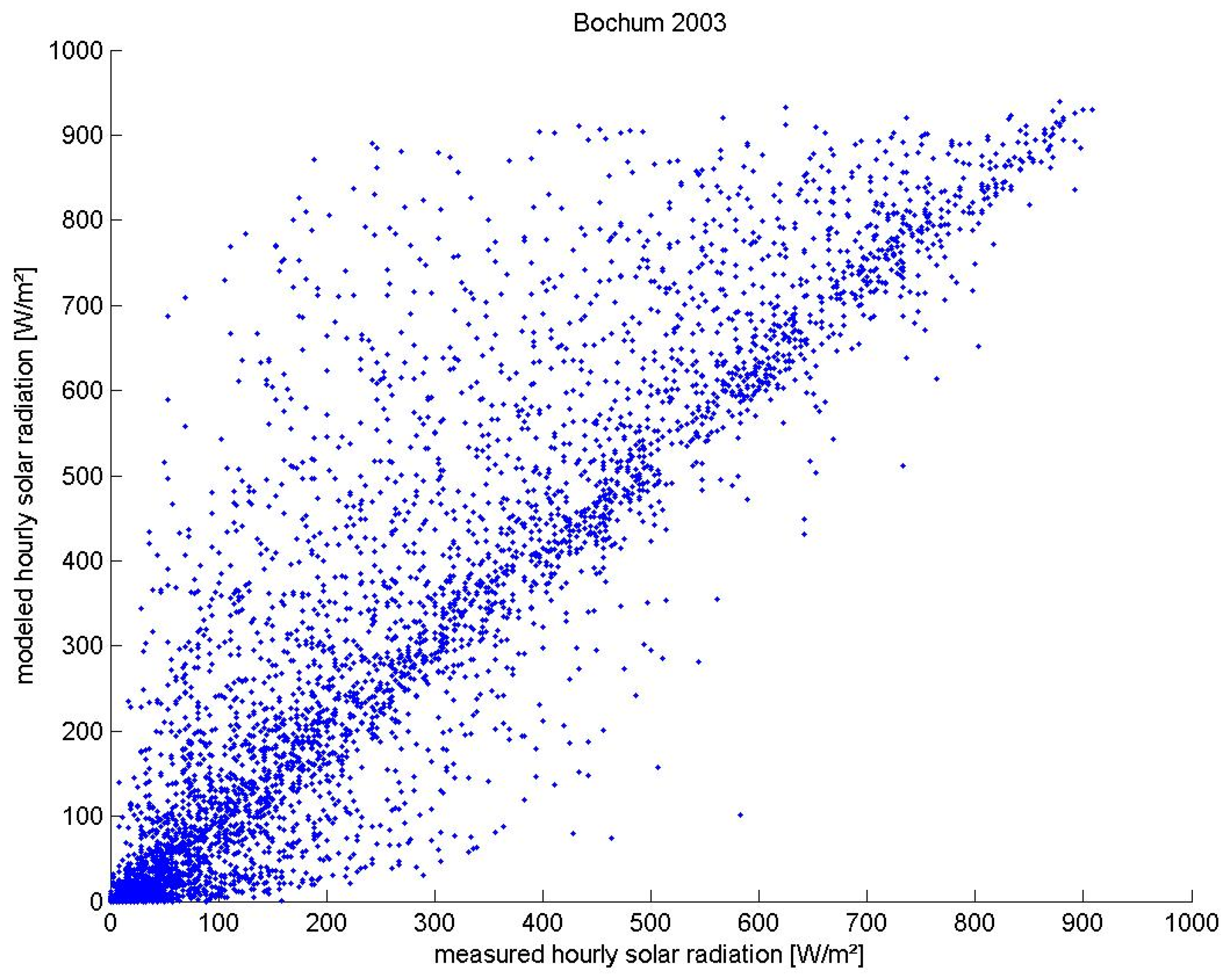
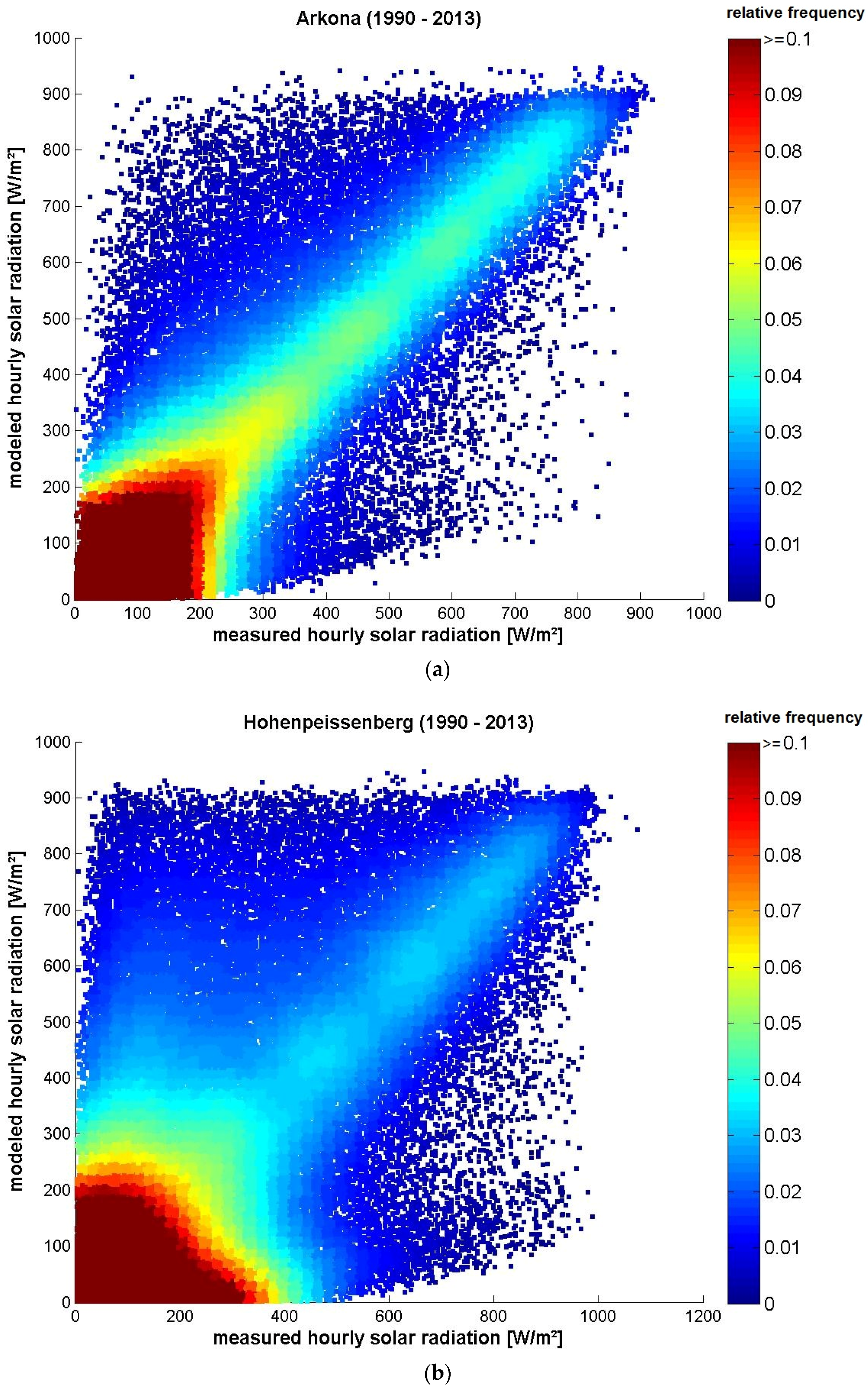
In order to visualize the linear correlation between the data sets we generated two illustrative density scatterplots (Figure 3). While the correlation between the data sets is recognizable there are a considerable number of events when measured and modeled values differ substantially. The trend of systematic higher model values, measured by the MBE, can also be observed in the density scatterplots by the high number and higher intensity of pixels above the 45° line. Altogether we conclude that the mean correlation coefficient of 90% indicates a decent model performance, although some of the authors presented in Section 2 find a higher correlation between the model and measurement data subject to their study.
Figure 3. Illustrative density scatterplots showing measured and modeled data (hourly) for two sites at Arkona with the highest correlation (a) and Hohenpeissenberg with the lowest (b).
Atmosphere 06 01835 g003
Summarizing the findings above about MBE, RMSE and R, two main reasons become evident why the previously calculated indicators are not sufficient for an assessment of the model’s performance in simulating irradiation data:
Firstly, they contradict each other and produce different rankings of performance. While on average the model shows a high MBE, the RMSE appears to be within the limits of a good model performance. Looking at the site “Hohenpeissenberg”, we find the lowest MBE of all considered measurement stations 0.4 W/m2 and 0.3%. However, the RMSE is only about average with 104 W/m2 and the correlation coefficient R is the lowest of all stations. These indicators by themselves appear to be insufficient to assess a model’s performance as also remarked by other authors (e.g., [6]).
Secondly, the above calculated indicators do not capture the relevant properties of an irradiation time series when doing analysis of decentralized energy systems. They look for the degree of similarity between measured and modeled data but not for the ability to simulate fluctuations and extreme values as realistic as possible. When doing energy systems analysis it is not crucial to forecast or reproduce weather time series as identical as possible. In fact, it is more important for the model output to capture the relevant characteristics of a time series (e.g., extreme values and gradients) and reproduce those in a realistic manner. Relevant characteristics identified in this work are the maximum amplitudes, gradients and the spatial volatility. They are important since they determine fundamental attributes of an energy system. For example the necessary grid capacity, the demand for flexible back-up generation capacity and its distribution within the grid.
In the following we summarize the results from applying the new indicators MARS, MGRS and the spatial volatility introduced in Section 3.2. These indicators are designed to capture and compare the fluctuations and volatile character of time series which are particularly important for energy systems analysts.

4.2. MARS, MGRS and Spatial Volatility

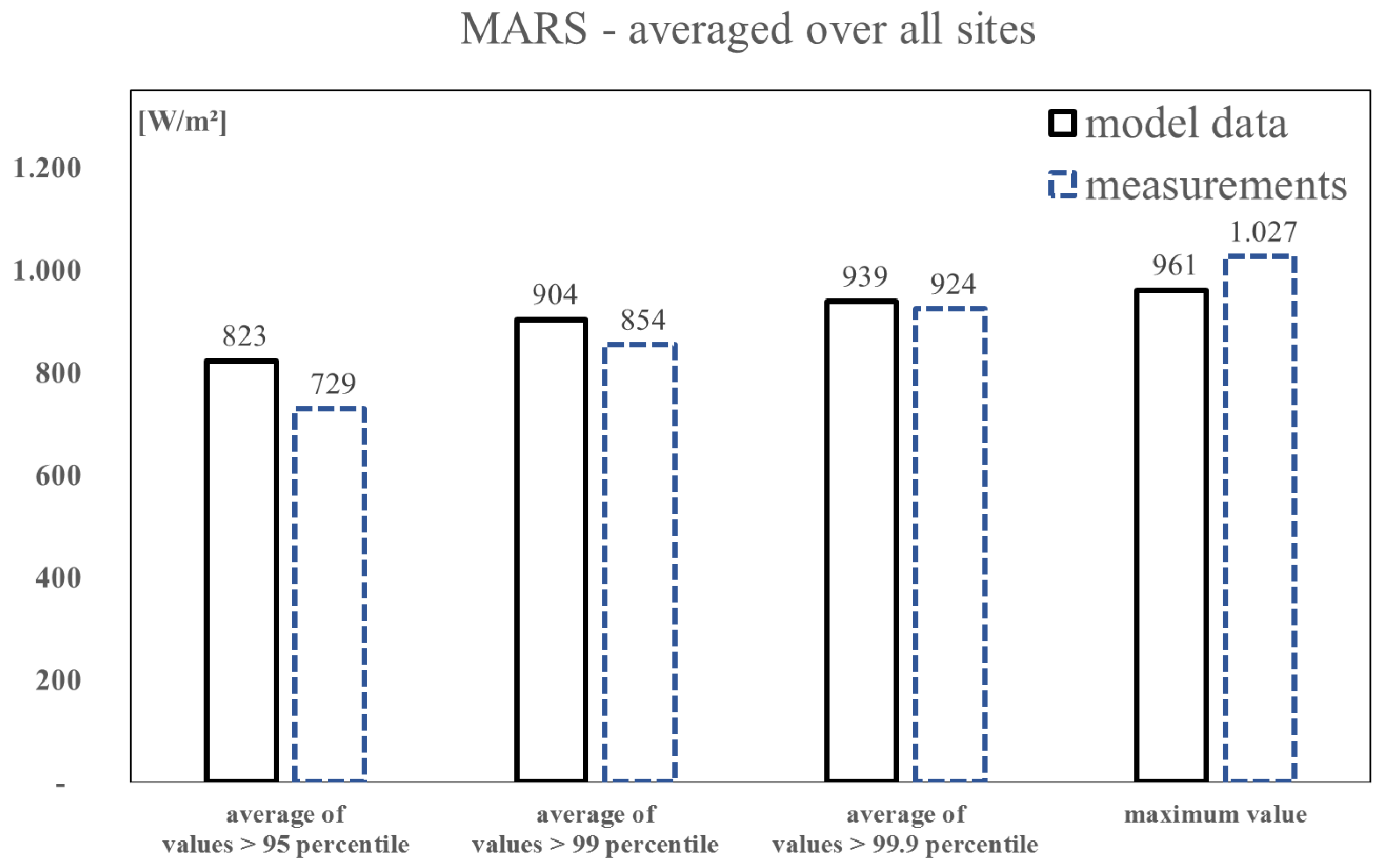
The maximum amplitude of irradiation supply (MARS) quantifies the level of solar irradiation during those hours of a time series with the highest supply. In energy systems analysis this is a valuable information since the fluctuating feed-in of solar irradiation driven generation units into the electricity grid is a major challenge for the operation and dimensioning of an energy system, especially on the decentralized level. The mean of the irradiation values greater than the 95, 99 and 99.9 percentile can be studied in Figure 4. Each of them separately calculated for the modeled and measured data and averaged over all available sites.
Figure 4. Maximum amplitude of irradiation supply (MARS) for different percentiles.
Atmosphere 06 01835 g004
On average the 5% largest values of the modeled data are 94 W/m2 or 12.9% higher than the equivalents of the measured data. This difference decreases to 50 W/m2 and 15 W/m2 when only the 1% largest and 0.1% largest values are taken into account. In other words, during one year with 8760 h the model data exceed the measurements within 88 h representing the 99 percentile value and higher (9 h being the 99.9 percentile and higher) by 5.8% (1.6%). Not surprisingly, this trend inverts when looking at the single largest value of each time series: The measurements are more vulnerable to errors and at the same time capture extreme and rare events at a single site, whereas the model simulates irradiation data averaged over a larger area. As a result, the maximum value of the model data is 66 W/m2 or 6.4% lower than the measurement data’s maximum.
In order to assess the results of the MARS we compare it to the results of the RMSE, which represents an indicator for the scattering of data and which is normalized to the range of the measured data. The differences between the MARS95 of modeled and measured data is lower than 13% or 100 W/m2. Regarding the extreme hours of highest supply (MARS99 and MARS99.9) the difference is well below 10% while the RMSE of the data sets averages to 11% and 108 W/m. Comparing to the RMSE, the MARS reveals a rather positive indication for the model’s performance in simulating extreme high values of solar irradiation. This particularly holds when taking into account the model’s exceedance of irradiation supply revealed by the MBE.
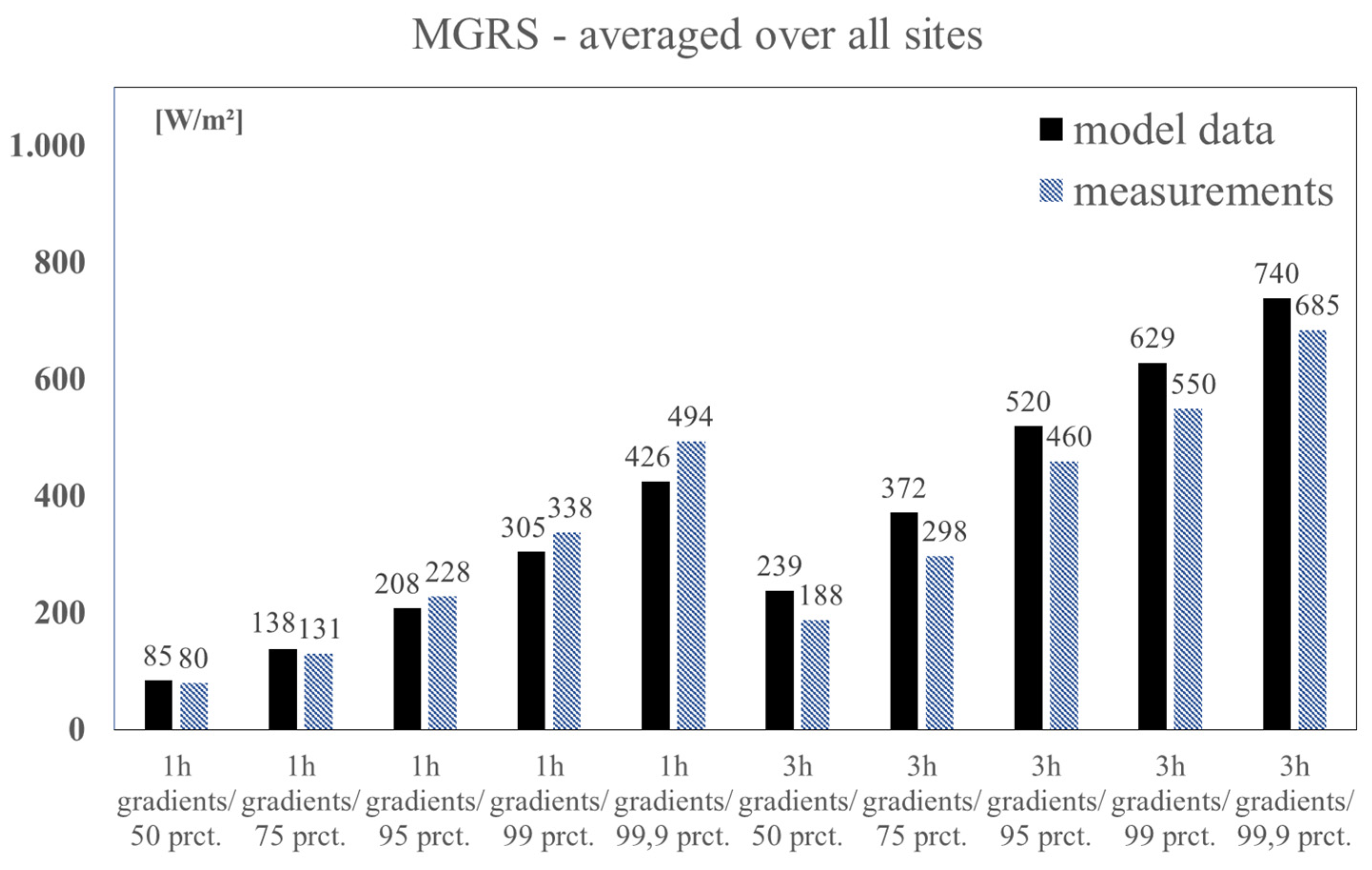
The maximum gradient of irradiation supply (MGRS) is also calculated for different percentiles and presented in Figure 5. It measures the change rate of the irradiation supply within a determined time span. In this paper, we calculate the MGRS on the level of 1 h and 3 h intervals. A higher resolution in time (e.g., 10 min) would be interesting to look into, but the available measurement data is limited to hourly values.
Figure 5. Maximum gradient of irradiation supply (MGRS) for different percentiles.
Atmosphere 06 01835 g005
The MGRS within 1 h varies from 208 to 494 W/m2 for the values greater than the 95-percentile. This corresponds to a change of irradiation supply between 21% and 50%, relative to the maximum value of solar irradiation supply of 994 W/m2, averaged over the model and measurement data of all stations. On the level of single stations the MGRS of model and measurement data varies by a standard deviation of 15–93 W/m2 for the 3-h MGRS and 6–128 W/m2 for the 1-h MGRS (strictly monotonic increasing with the percentile, except for the 99,9 percentile of the 3 h gradients). Looking at the 3 h intervals, the MGRS95, MGRS99 and MGRS99.9 vary between 46% and 74% of the maximum solar irradiation value. As expectable the MGRS within 3 h is significantly greater than within 1 h.
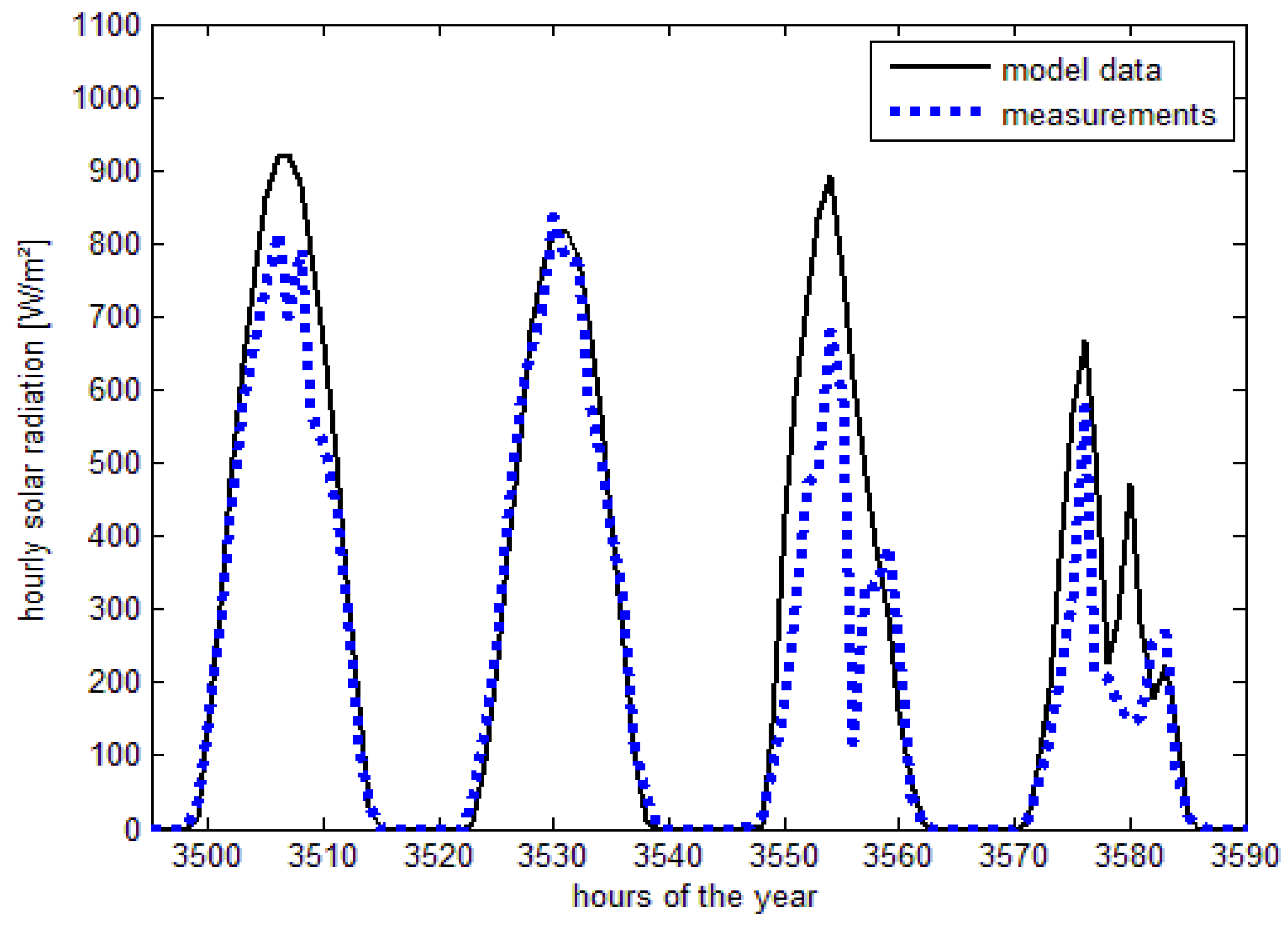
Studying the 1 h-gradients, it strikes one that the gradients of the measurement data above the 95 percentile are greater than those of the model data but for the lower percentiles this trend reverses. This may be explained looking at Figure 6: As mentioned before, each measured time series represents the irradiation supply of a single location in contrast to the model data which simulates a larger area. A single cloud shadowing the measurement station might result in a high MGRS for the measured data but not necessarily on the aggregated level represented by the model data. The results from the MGRS suggest that the measurements at single locations show higher fluctuations than the model data representing irradiation over an area.
Figure 6. Illustrative excerpt from the irradiation time series (station: Aachen).
Atmosphere 06 01835 g006
However, when regarding lower percentiles (e.g., 75 and 50) the model data shows higher average gradients. This might be interpreted as follows: The very high fluctuations on the hourly level appear infrequently, which can be derived from the strong decrease in the MGRS at lower percentiles. Therefore, the highest gradients are not caused by the hours around daily sunrise and sunset but by changes in cloud coverage during the day leading to large fluctuations in irradiation supply. Taking more values into account by applying lower percentiles, the daily gradients in the morning and afternoon gain more and more influence on calculating the average gradient and result in a higher model-MGRS. Evidently, the model simulates the hours around sunrise and sunset with a higher gradient than observed by the measurement stations.
At the temporal resolution of 3 h gradients, the model data generally exhibits larger gradients. The MGRS95, MGRS99 and MGRS99.9 exceed the measurement’s MGRS by about 10%. We conclude that at the 3 h resolution the strong diurnal fluctuations of the measurement data due to cloud coverage mentioned above, disappear against the daily gradients of sunrise and sunset. As already discovered from the 1 h gradients, the modeled deterministic changes in the morning and in the evening hours possess a higher gradient as the measurements.
In order to evaluate the results of the MGRS we calculate the respective standard deviation of model and measurement data since it is a well-known indicator for the fluctuation of a time series. For the model and measurement data respectively, it amounts to 242 W/m2 and 198 W/m2 averaged over all sites. Derived from the MGRS95 to MGRS99.9, the model underestimates the hourly gradients by 9% to 14% or 20 to 69 W/m2. For the 3 h gradients, the same MGRS percentiles correspond to an overestimation of 8% to 14% or 54 W/m² to 79 W/m2. Compared to the difference between the standard deviations of 44 W/m2, the differences in MGRS appear to be within acceptable limits. This is confirmed regarding the RMSE between the data sets which lies within a similar scale of 11% or 108 W/m2 (compare Section 2).
It becomes clear that the main differences between the fluctuations of the two data sets arise firstly from the gradient of solar irradiation supply during the hours of sunrise and sunset and secondly from abrupt diurnal changes in cloud coverage. While the first factor might result from a model weakness, we relate the second factor to the difference between modeling the solar irradiation supply received by a whole area and measurements taken at a single site. From the authors’ point of view the 1h-gradients are rather relevant for energy systems analysis, since they are dominated by non-deterministic, diurnal fluctuations.
The concept of the spatial volatility is to measure the spatial differences of solar irradiation supply and thereby the difference in possible RES-E generation in space. It is an indicator for regional disparities in solar irradiation supply caused by the deterministic ecliptic of the sun on the one hand and stochastic spatial weather variety on the other hand.
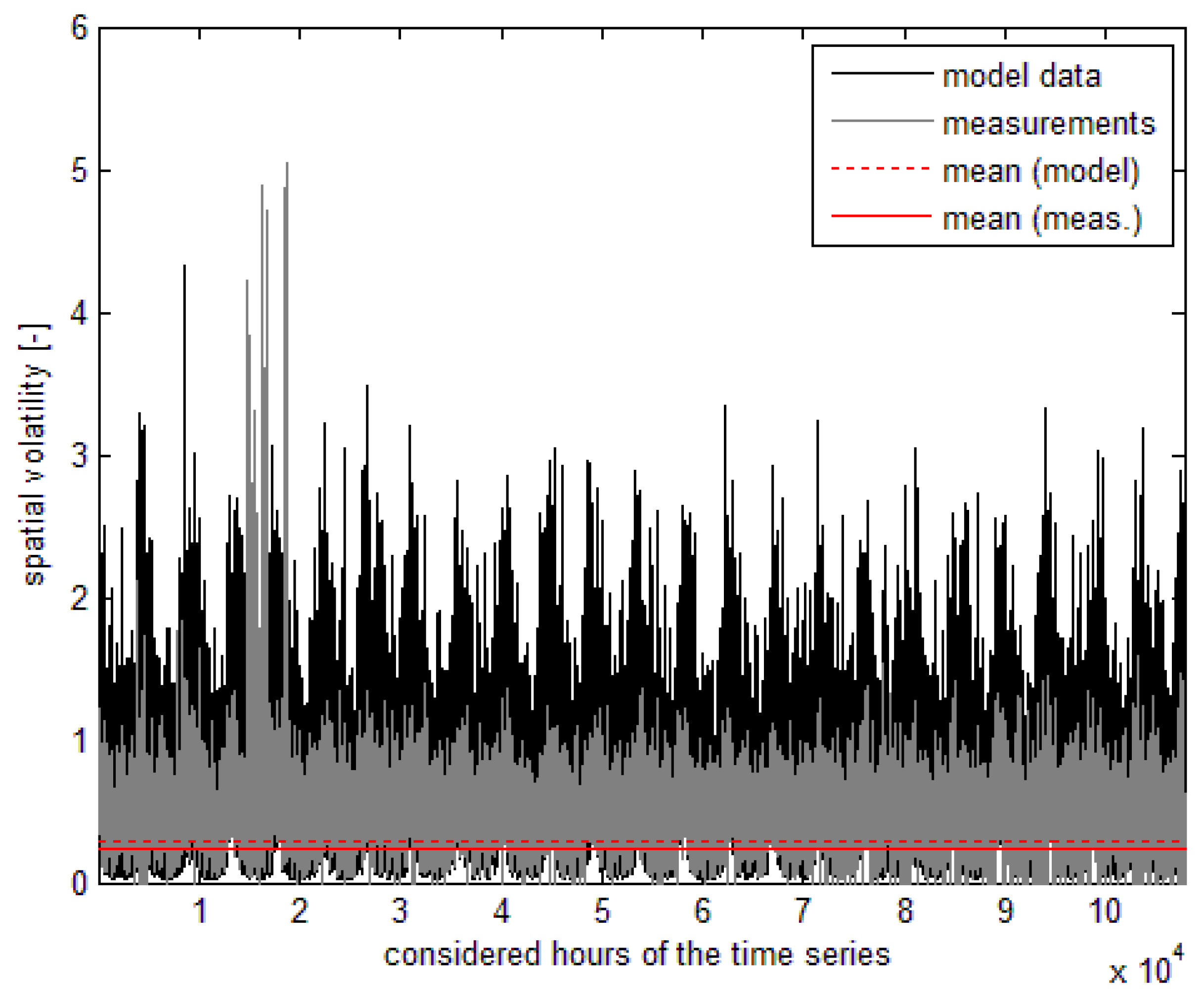
The respective spatial volatility of the model data and the measurements are depicted in Figure 7. The calculation of the spatial volatility considers only those hours of the 24 years that have a solar irradiation greater than zero (hours with no irradiation are excluded). For every analyzed time step there was data available from at least 29 of the 57 measurement stations.
Figure 7. Spatial volatility of the measured and modeled data respectively.
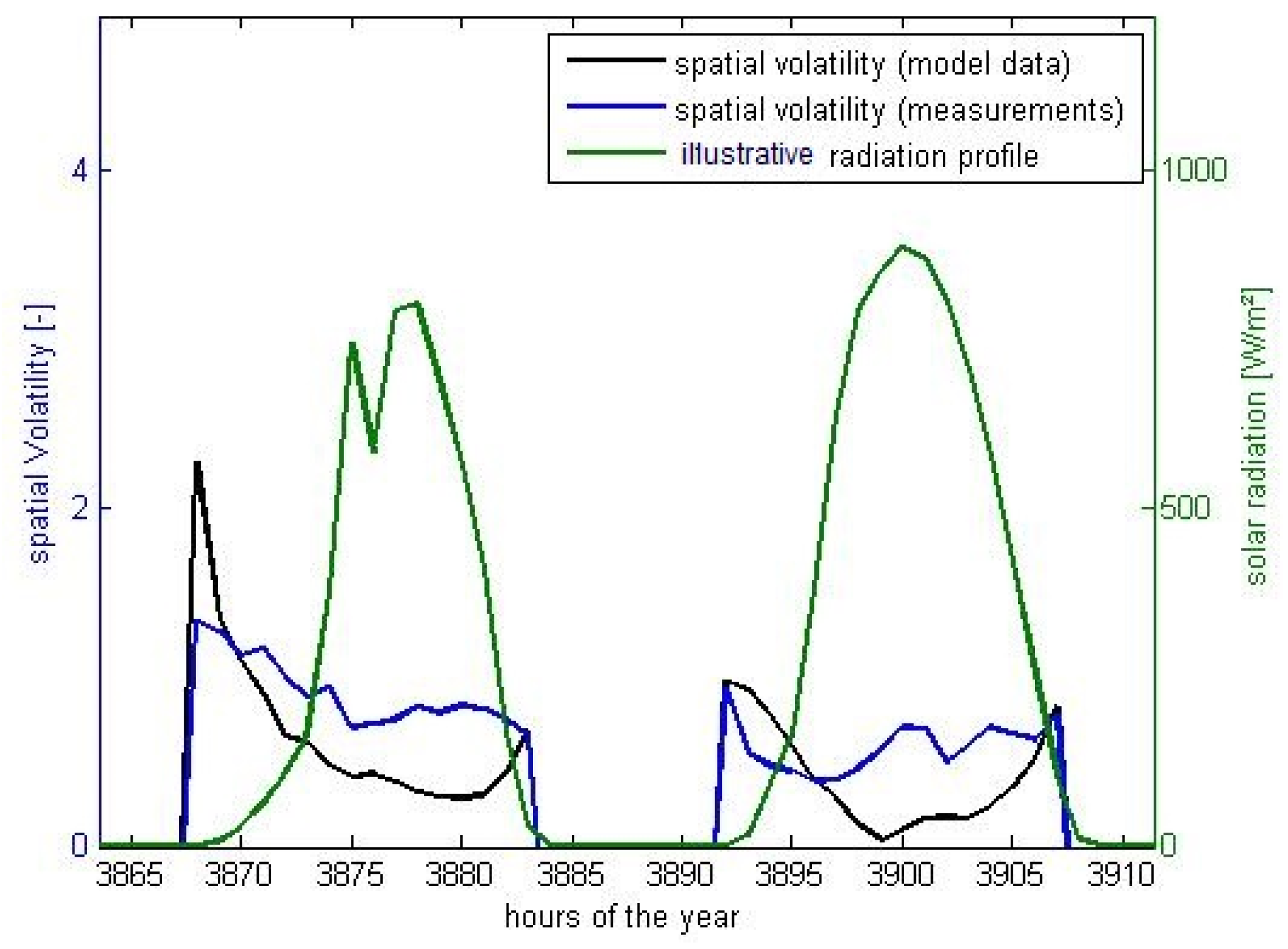
Atmosphere 06 01835 g007
Figure 8. Spatial volatility of the measured and modeled data on two illustrative days.
Atmosphere 06 01835 g008
At first glance, it seems that the model’s spatial volatility exceeds the measurement’s spatial volatility because of its frequent positive spikes. However, the spatial volatility of the model data averages 29% and is only slightly higher than the measurement’s mean spatial volatility of 24%. In fact, taking a closer look at the time series (Figure 8) it unfolds that during the day, the spatial volatility of the measurement stations is regularly higher than the model’s spatial volatility.
This goes along well with the results from the MGRS assessment, where we found on the hourly level that the gradients of the model are higher during the hours of sunrise and sunset but lower during the day compared to the measurements from single sites. In Figure 8, we find a similar trend: The model produces a rather high spatial volatility during the morning and afternoon hours compared to the measurement data. During the day this trend reverses. However, both modeled and measured time series generally produce higher spatial volatility during the hours of sunrise and sunset compared to midday. This seems reasonable since the spatial distribution of the 57 sites, particularly along the longitudes, is accompanied by differences in their respective position to the sun. This results in additional variations during those hours.
Taking into account the above mentioned arguments the spatial volatility does not deliver a definite judgment of the model’s performance. However, it produces valuable information about the spatial fluctuations of irradiation supply during the day, consistent for both modeled and measured data. The spatial volatility also identifies the hours of sunset and sunrise as particular critical with respect to interregional fluctuations of RES-E feed-in and delivers a quantifying indicator.

4.3. Critical Appraisal

Applied to the data set, the spatial volatility reveals substantial differences between modeled and measured data (the model data’s spatial volatility exceeds the measurement data’s by 5 percentage points, which is 21% more). This appears to be a rather high difference and might be explained by methodical differences in the data formats and temporal resolution of time stamps within the data sets: Since the measurement data are administrated using the ‘apparent local time’, it was necessary to convert the time stamps of the data of every single location allowing for temporal shifts of up to one hour. While the model data is available at a resolution of 10 min, the measurement data was only available on an hourly basis. This inevitably leads to an inaccurate conversion of temporal differences. The conversion algorithm for the time stamps of the measurement data used in this work can be considered as underestimating the spatial volatility. Therefore, the observed difference in the spatial volatility between model and measurement data is rather overestimated.
For future development of the MARS, MGRS and spatial volatility introduced in this paper, it might prove helpful to eliminate deterministic trends of the solar irradiation time series. Thus, frequent and repetitive changes in irradiation supply that are easier to predict do not affect the indicators. Moreover, a higher temporal resolution will help to improve the significance of the MARS, MGRS and spatial volatility. This would enable a more accurate preprocessing of the data on the one hand and allow conclusions on the higher temporal resolution on the other hand.

5. Conclusions and Outlook

The goal of this paper is the evaluation of existing and the development of new performance indicators for the assessment of data output from a numerical weather model in the context of decentralized energy systems.
From literature, we extract three first order statistics indicators that aggregate information from comparing two time series: MBE, RMSE and R. Applying them on the historic data from 57 measurement stations and corresponding model data, they produced an inconsistent assessment result. More importantly, they did not measure the relevant properties of the time series when analyzing decentralized energy systems. Grid constraints caused by RES-E mainly occur on a decentralized level and can only be simulated appropriately if extreme and rare values of solar irradiation and fluctuations of the irradiation supply in space and time are modeled in a realistic way. In order to measure these relevant characteristics, we introduce the MARS, MGRS and the spatial volatility and apply these to the data set.
Calculating the MARS shows a good performance of the model with respect to reproducing very high irradiation values, even though the model tends to overestimate the amplitudes. Suggesting larger maximum capacities of RES-E feed-in, this overestimation potentially leads to an oversized grid capacity which might be welcomed from a risk-averse perspective.
Evaluated by the 3 h and the 1 h MGRS, the model’s performance qualifies as moderate compared to the standard deviation and the RMSE. The model’s overestimation of the 3 h gradients tends to recommend an excess supply of flexible generation capacity. Again, from a risk-averse perspective this might be welcomed. The underestimation of the differences between the 1 h gradients can convincingly be attributed to the systematic differences of measurements at a single site and the modeling of a larger area. Measurements at a single location capture every cloud reducing irradiation supply whereas the model data might allow for balancing effects within one ‘weather cell’. When analyzing energy systems with some regional extent, it is likely for balancing effects between photovoltaics and other RES-E generation units to occur. Therefore, the model’s lack of ability to reproduce high diurnal gradients and spatial fluctuation appears to be a more realistic simulation of the solar irradiation supply received by an underlying energy system.
The spatial volatility proves to be an effective tool to measure regional differences of RES-E generation potential. It quantifies diurnal spatial fluctuations of irradiation supply and identifies the hours of sunset and sunrise as particular critical with respect to interregional fluctuations. Both MGRS and the spatial volatility capture the systematic difference between the different spatial resolutions of the data sets quite well. From the novel indicators introduced in this paper, the spatial volatility promises the most potential for future development. For example, a further improvement of data input or a thorough investigation of diurnal and geographic patterns of the spatial volatility appear as promising enhancements of the spatial volatility’s findings.
The indicators MARS, MGRS and spatial volatility present instruments for energy systems analysts to quantify the need for flexible capacities to balance out the fluctuating renewable supply in time. They also allow us to draw conclusions about the spatial differential in renewable energy supply and thus electricity grid dimensioning.

Acknowledgments

This paper is partially based on research conducted within the project “Dezentrale Energiesysteme, Marktintegration und Optimierung(DEMO) at KIT. The authors gratefully thank the “Stiftung Energieforschung Baden-Württemberg” for the financial support. The authors also thank the German National Meteorological Service (DWD) for the delivery of the measurement data. We acknowledge support by Deutsche Forschungsgemeinschaft and Open Access Publishing Fund of Karlsruhe Institute of Technology.

Author Contributions

Hans Schermeyer designed this study, conducted the analysis, interpreted the data and wrote the manuscript. Valentin Bertsch and Wolf Fichtner contributed to the data interpretation, provided important suggestions and improved the manuscript.

Conflicts of Interest

The authors declare no conflict of interest.

References

  1. Schermeyer, H.; Bertsch, V.; Fichtner, W. Validation and utilization of numerical weather model data in energy systems analysis of decentralized electricity production. In Proceedings of the 7th International Scientific Conference on Energy and Climate Change, Athens, Greece, 8–10 October 2014.
  2. MM5 Community Model Homepage, Modeling System Overview. Available online: http://www2.mmm.ucar.edu/mm5/overview.html (accessed on 16 May 2014).
  3. Murphy, A.H. The Coefficients of correlation and determination as measures of performance in forecast verification. Wea Forecast. 1995, 10, 681–688. [Google Scholar] [CrossRef]
  4. Myers, D.; Wilcox, S.; Marion, W.; George, R.; Anderberg, M. Broadband model performance for an updated National Solar Radiation Database in the United States of America. In Proceedings of the Solar World Congress 2005, Bringing Water to the World, Orlando, FL, USA, 8–12 August 2005.
  5. Polo, J.; Zarzalejo, L.; Ramírez, L. Solar Radiation Derived from Satellite Images. In Modeling Solar Radiation at the Earth’s Surface; Badescu, V., Ed.; Springer: Berlin, Germany, 2008; pp. 449–462. [Google Scholar]
  6. Gueymard, C.; Myers, D. Validation and Ranking Methodologies for Solar Radiation Models. In Modeling Solar Radiation at the Earth’s Surface; Badescu, V., Ed.; Springer: Berlin, Germany, 2008; pp. 479–510. [Google Scholar]
  7. Badescu, V.; Gueymard, C.A.; Cheval, S.; Oprea, C.; Baciu, M.; Dumitrescu, A.; Iacobescu, F.; Milos, I.; Rada, C. Computing global and diffuse solar hourly irradiation on clear sky. Review and testing of 54 models. Renew. Sustain. Energy Rev. 2012, 16, 1636–1656. [Google Scholar] [CrossRef]
  8. Huld, T.; Müller, R.; Gambardella, A. A new solar radiation database for estimating PV performance in Europe and Africa. Sol. Energy 2012, 86, 1803–1815. [Google Scholar] [CrossRef]
  9. Ineichen, P. Long Term Satellite Hourly, Daily and Monthly Global, Beam and Diffuse Irradiance Validation. In Interannual Variability Analysis; International Energy Agency: Geneva, Switerzland, 2013. [Google Scholar]
  10. Liebenau, V.; Schwippe, J.; Kuch, S.; Rehtanz, C. Network extension planning considering the uncertainty of feed-in from renewable energies. In Proceedings of the 2013 IEEE Grenoble PowerTech, Grenoble, France, 16–20 June 2013; pp. 1–6.
  11. IEA (2011): IEA/SHC Task 36 Solar Resource Knowledge Management. International Energy Agency. Available online: http://archive.iea-shc.org/publications/task.aspx?Task=36 (ascessed on 30 November 2015).
  12. Hoyer-Klick, C.; Beyer, H.-G.; Dumortier, D.; Schroedter Homscheidt, M.; Wald, L.; Martinoli, M.; Schillings, C.; Gschwind, B.; Ménard, L.; Gaboardi, E.; et al. MESoR—Management and exploitation of solar resource knowledge. In Proceedings of the SolarPACES 2009, Berlin, Germany, 15–18 Sptember 2009.
  13. Espinar, B.; Ramírez, L.; Drews, A.; Beyer, H.G.; Zarzalejo, L.F.; Polo, J.; Martín, L. Analysis of different comparison parameters applied to solar radiation data from satellite and German radiometric stations. Sol. Energy 2009, 83, 118–125. [Google Scholar] [CrossRef]
  14. Hoyer-Klick, C.; McIntosh, J.; Moner-Girona, M.; Renné, D.; Perez, R.; Puig, D. Developing a Guide for Non-experts to Determine the Most Appropriate Use of Solar Energy Resource Information. http://archive.iea-shc.org/publications/downloads/Developing_a_Guide_for_Non-expert_v0.9-20100707.pdf (ascessed on 30 November 2015).
  15. Ineichen, P. Five Satellite Products Deriving Beam and Global Irradiance Validation on Data from 23 Ground Stations; International Energy Agency: Geneva, Switzerland, 2011. [Google Scholar]
  16. Massey, F.J. The Kolmogorov-Smirnov test for goodness of fit. J. Am. Stat. Assoc. 1951, 46, 68–78. [Google Scholar] [CrossRef]

