
Wind Regimes above and below a Temperate Deciduous Forest Canopy in Complex Terrain: Interactions between Slope and Valley Winds


Abstract
:1. Introduction
2. Slope/Valley Wind Theory
3. Experimental Section
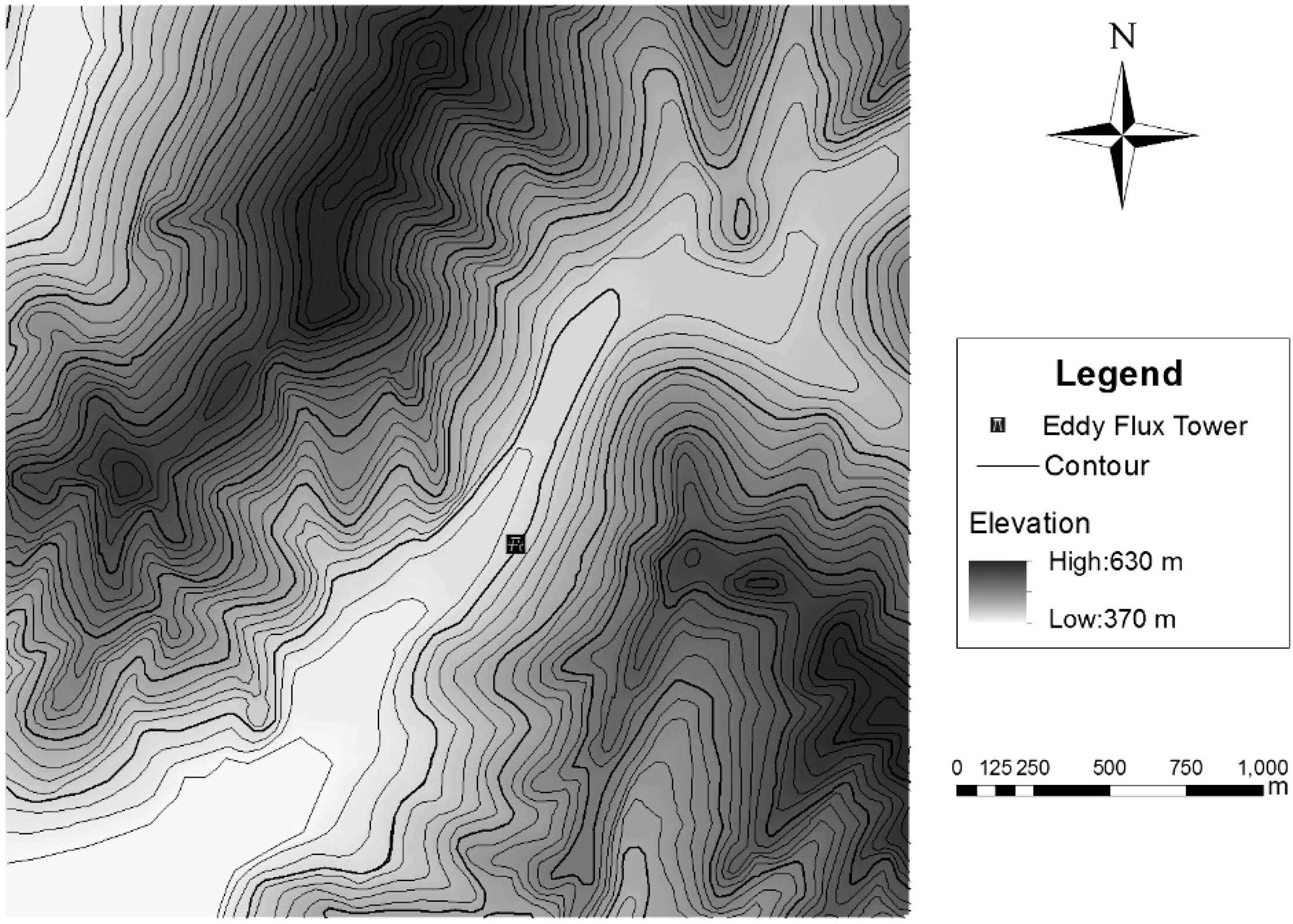
3.1. Site Description
3.2. Measurements and Instrumentations


| Variable | Height (m) | Anemometer Type | Instrument, Supplier |
|---|---|---|---|
| Horizontal wind velocity | 48, 42, 36, 28, 21, 16 | Cup | 010C, Met ONE |
| 2 | Sonic | 81,000, R.M. Yong | |
| Horizontal wind direction | 48 | Vane | 010C, Met ONE |
| 21 | Vane | 020C, Met ONE | |
| 2 | Sonic | R.M Young 81,000, R.M. Yong | |
| Vertical wind velocity | 36 | Sonic | CSAT3, Campbell Scientific |
| Net radiation | 48, 2 | - | CRN1, Kipp & Zone, |
| Air temperature and humidity | 48, 36, 28, 16, 2 | - | HMP45C with 076B, Vessla |
| Barometric pressure | 28 | - | CS100, Campbell Scientific |
3.3. Data Analysis
4. Results and Discussions
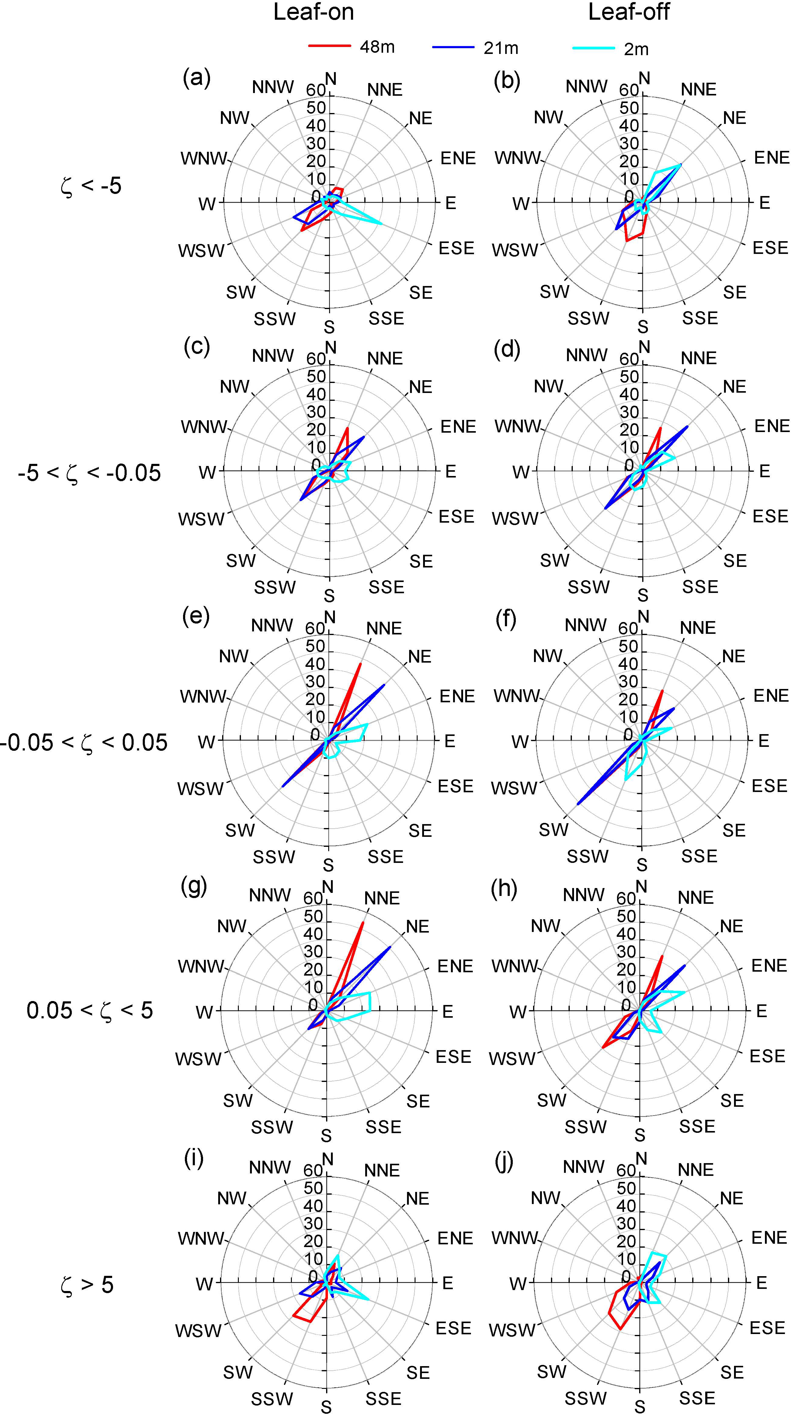
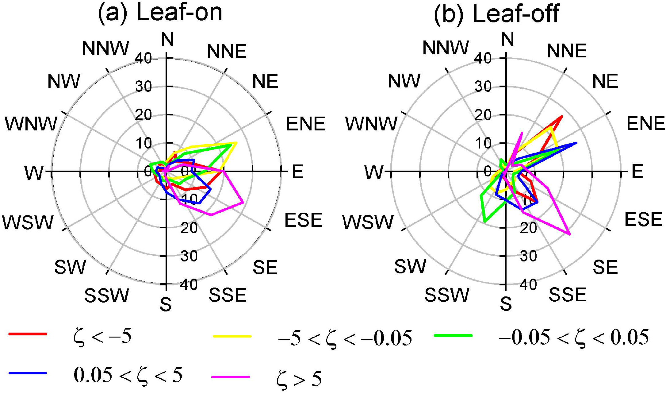
4.1. Variations in Wind Direction
4.1.1. Diurnal Variations in Wind Direction
| Measuring Height | Wind Direction | All Season | Leaf-on Season | Leaf-off Season | ||
|---|---|---|---|---|---|---|
| Day | Night | Day | Night | |||
| (m) | sector | (%) | (%) | (%) | (%) | (%) |
| 48 (above-canopy) | Down-valley | 44.4 | 30.1 | 77.3 | 21.5 | 51.1 |
| Down-slope | 8.9 | 16.0 | 6.1 | 6.2 | 7.6 | |
| Up-valley | 41.2 | 47.7 | 14.7 | 62.4 | 37.1 | |
| Up-slope | 5.5 | 6.3 | 1.9 | 9.9 | 4.1 | |
| 21 (just above canopy) | Down-valley | 45.6 | 27.8 | 73.6 | 21.5 | 58.1 |
| Down-slope | 10.3 | 11.5 | 14.4 | 6.2 | 10.0 | |
| Up-valley | 38.9 | 50.2 | 11.0 | 63.8 | 30.0 | |
| Up-slope | 5.3 | 10.5 | 1.0 | 8.6 | 2.0 | |
| 2 (under-canopy) | Down-valley | 21.7 | 7.7 | 29.5 | 9.5 | 35.6 |
| Down-slope | 53.4 | 56.7 | 62.7 | 35.7 | 57.1 | |
| Up-valley | 14.3 | 15.2 | 2.3 | 37.3 | 5.4 | |
| Up-slope | 10.7 | 20.4 | 5.6 | 17.5 | 1.9 | |
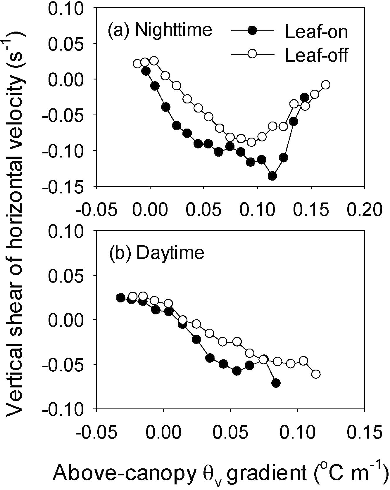
4.1.2. Vertical Shear of Wind Direction
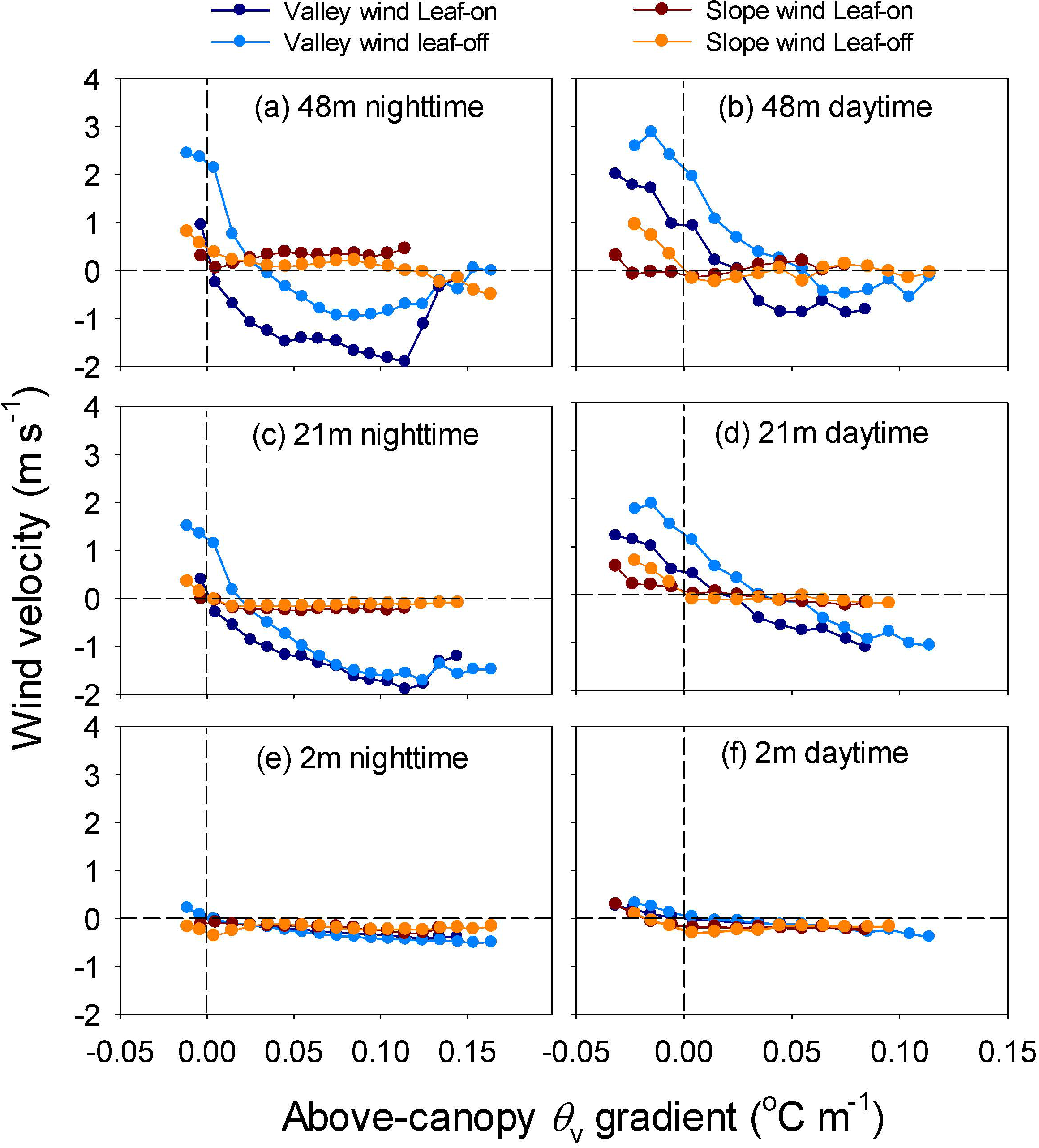
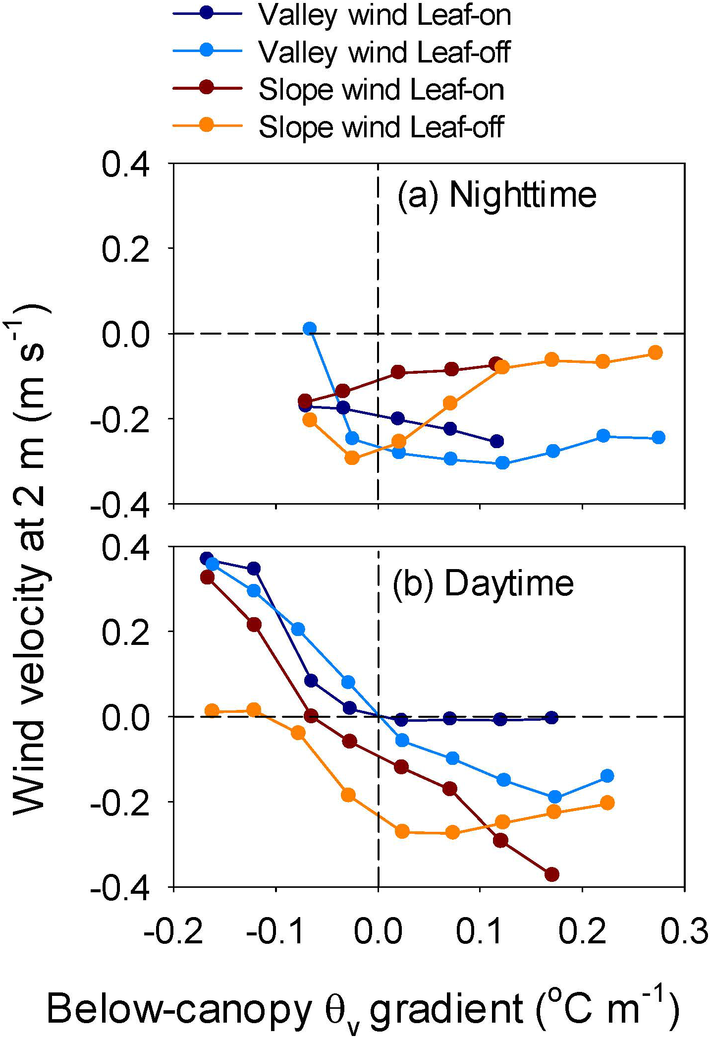
4.2. Variations in Wind Velocity
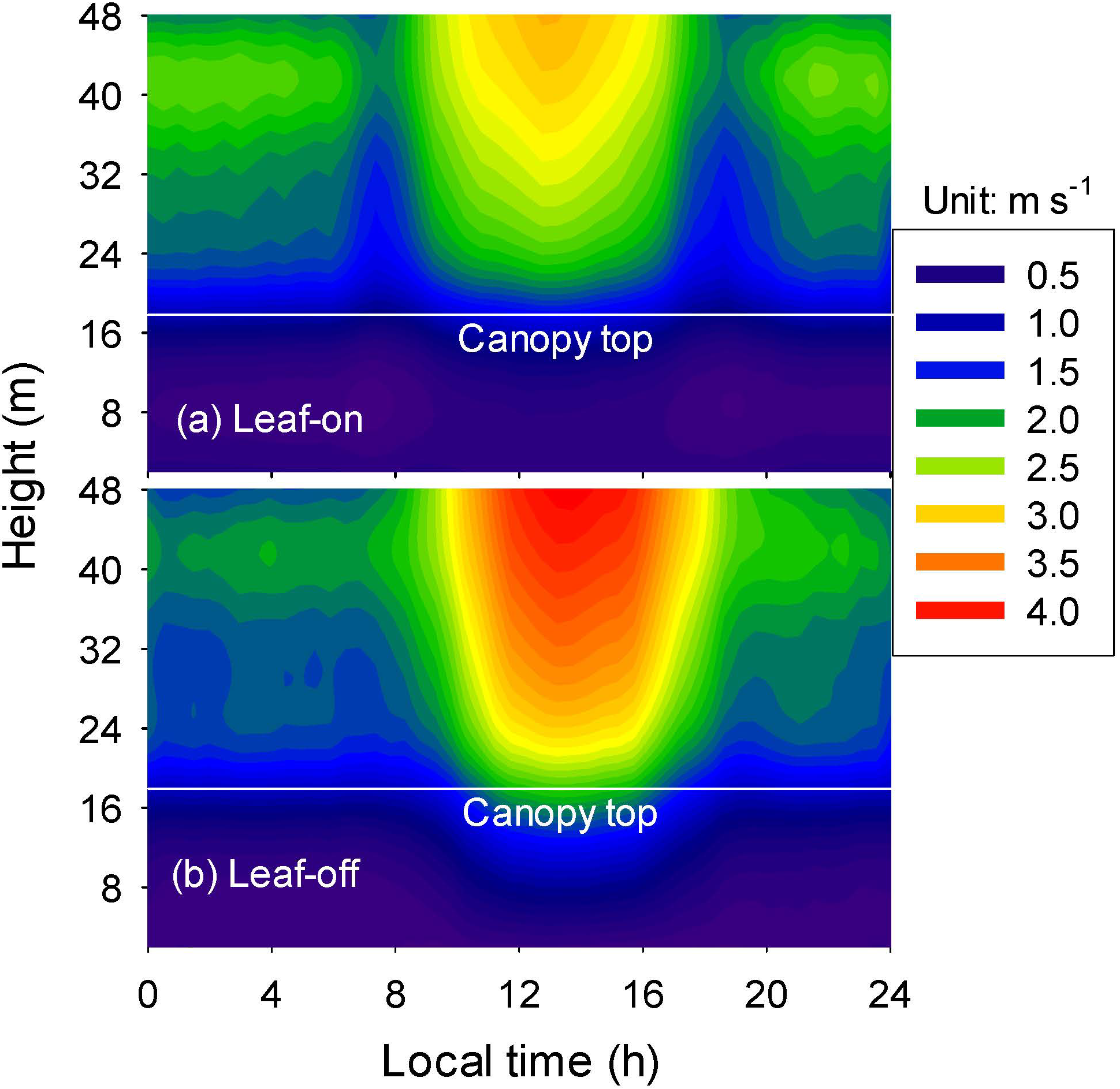
4.2.1. Horizontal Wind Velocity

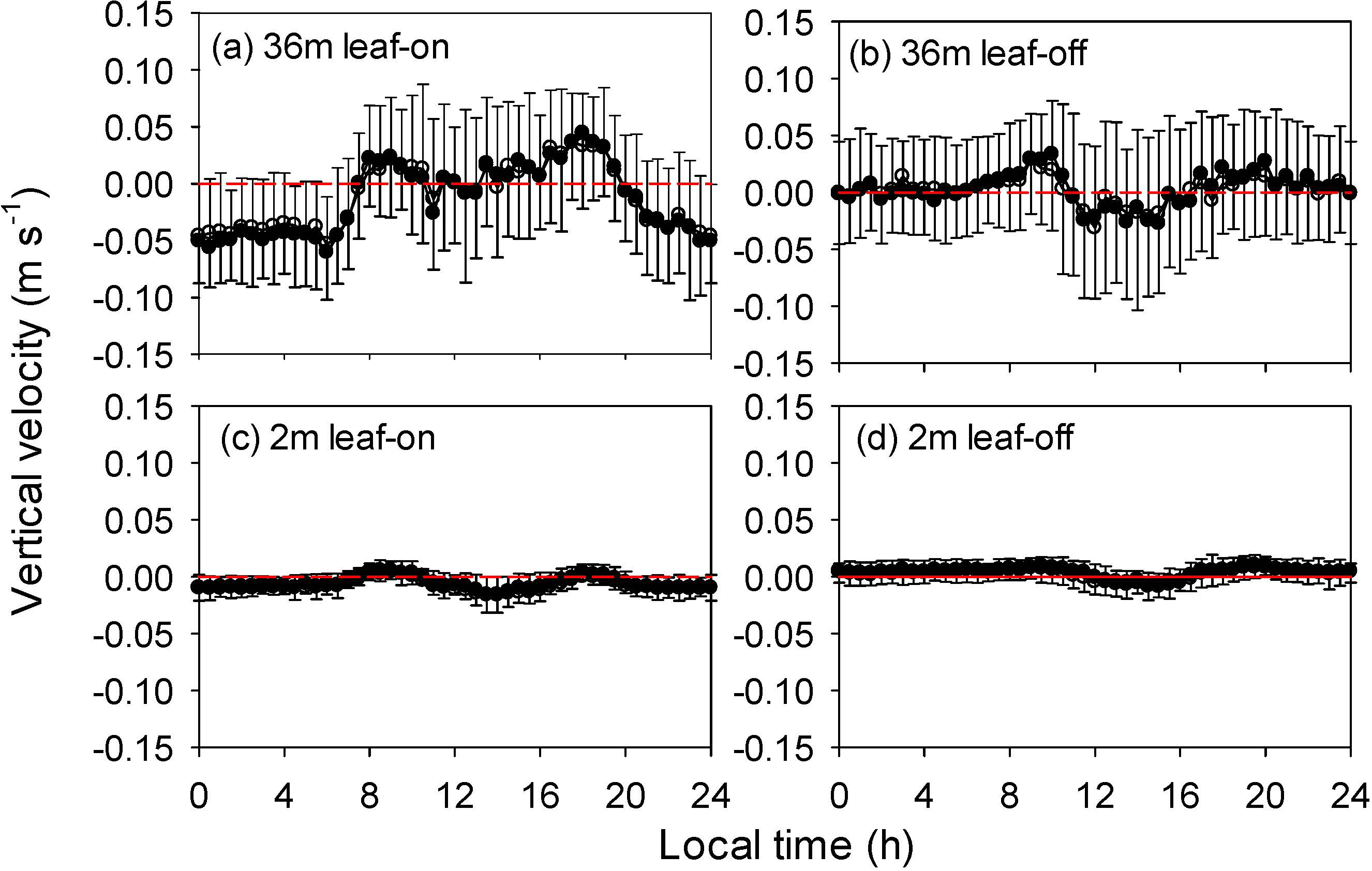
4.2.2. Vertical Wind Velocity

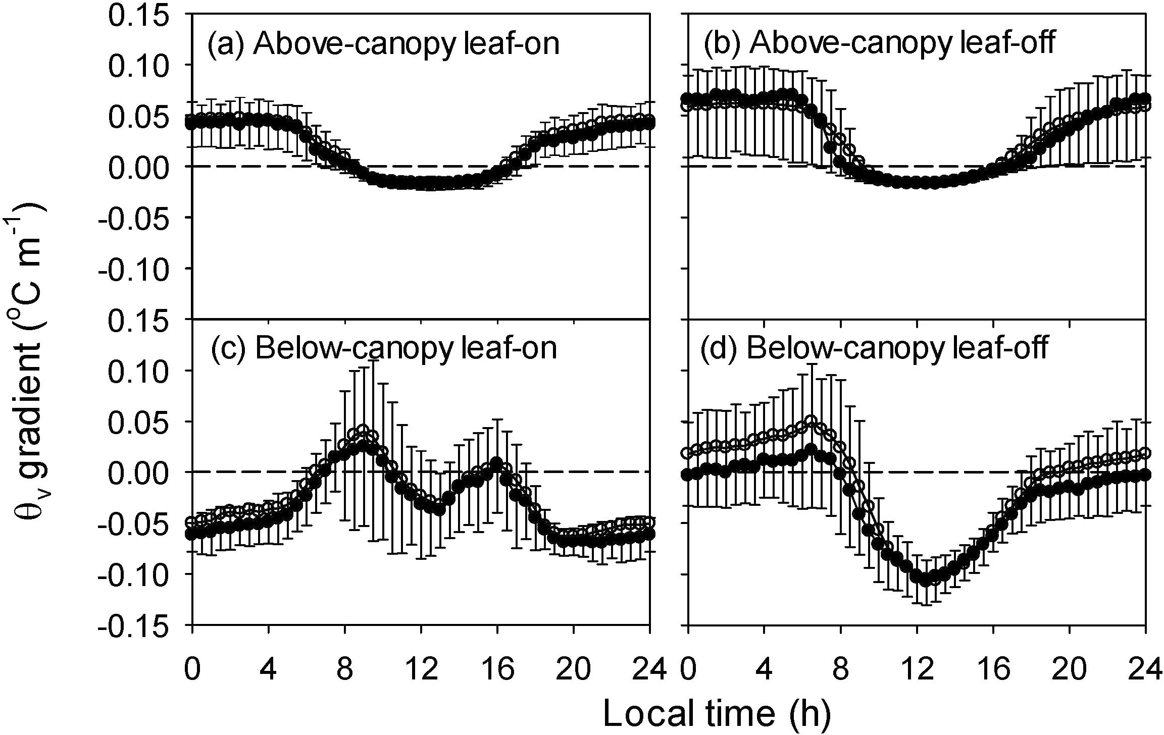
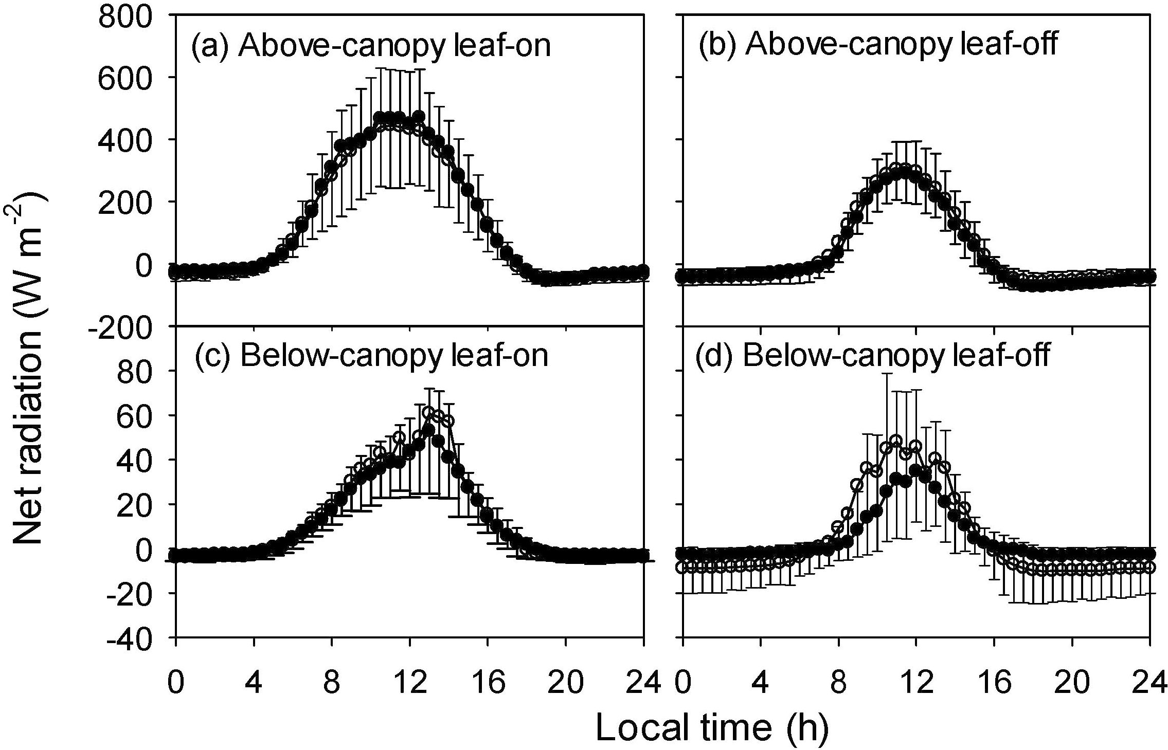
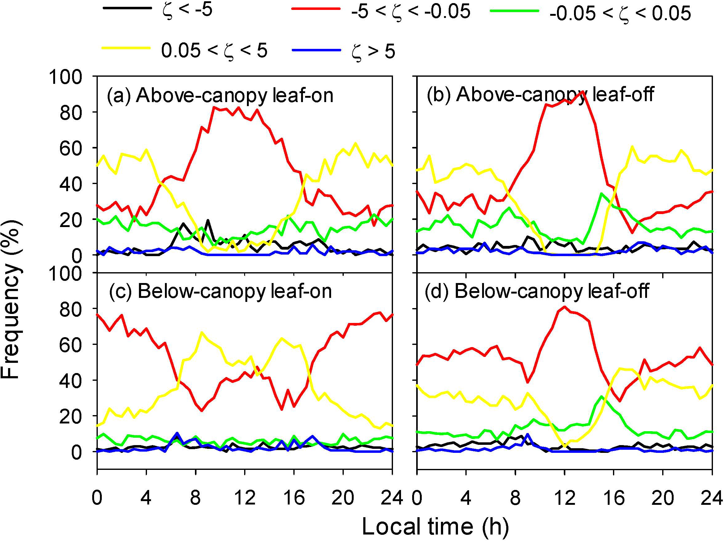
4.3. Variations in Thermal Gradient and Stability


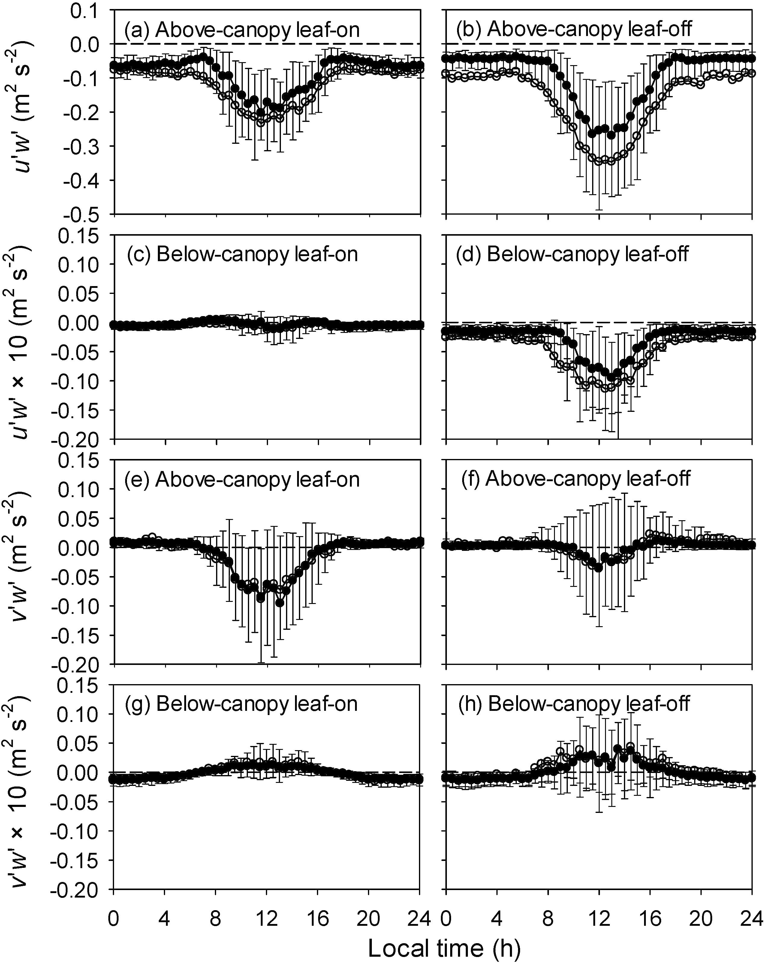
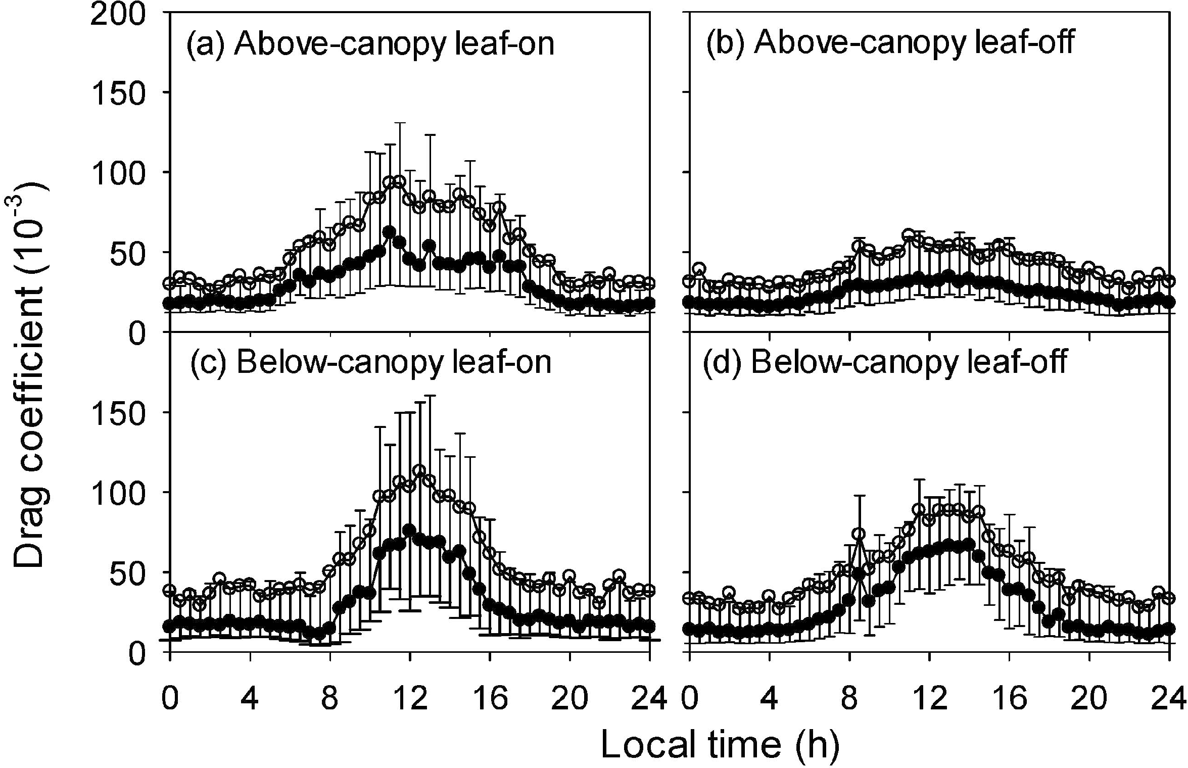
4.4. Variations in Reynolds Stress and Drag Coefficient

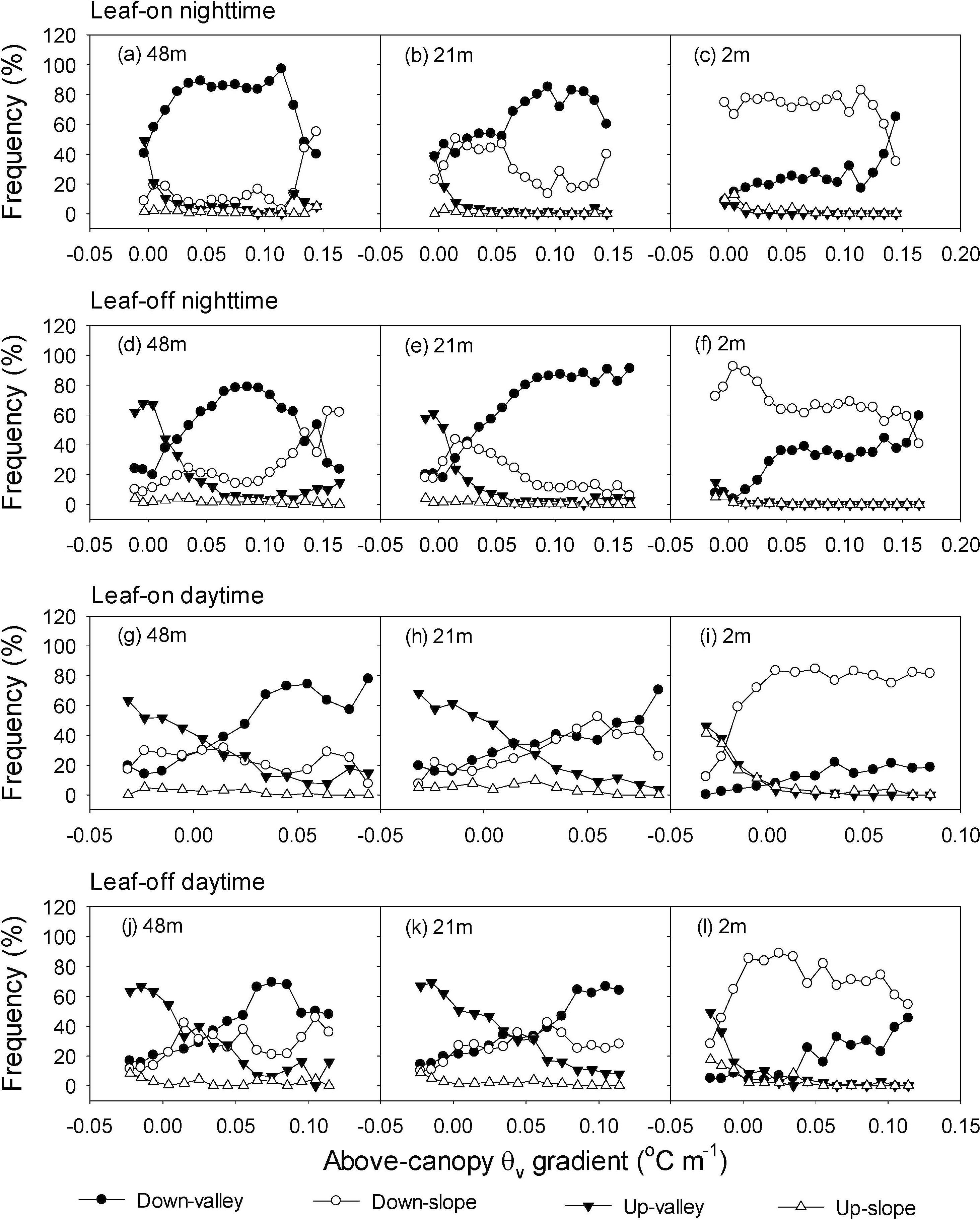
4.5. Relations to Thermal Gradient and Stability
4.5.1. Above-Canopy


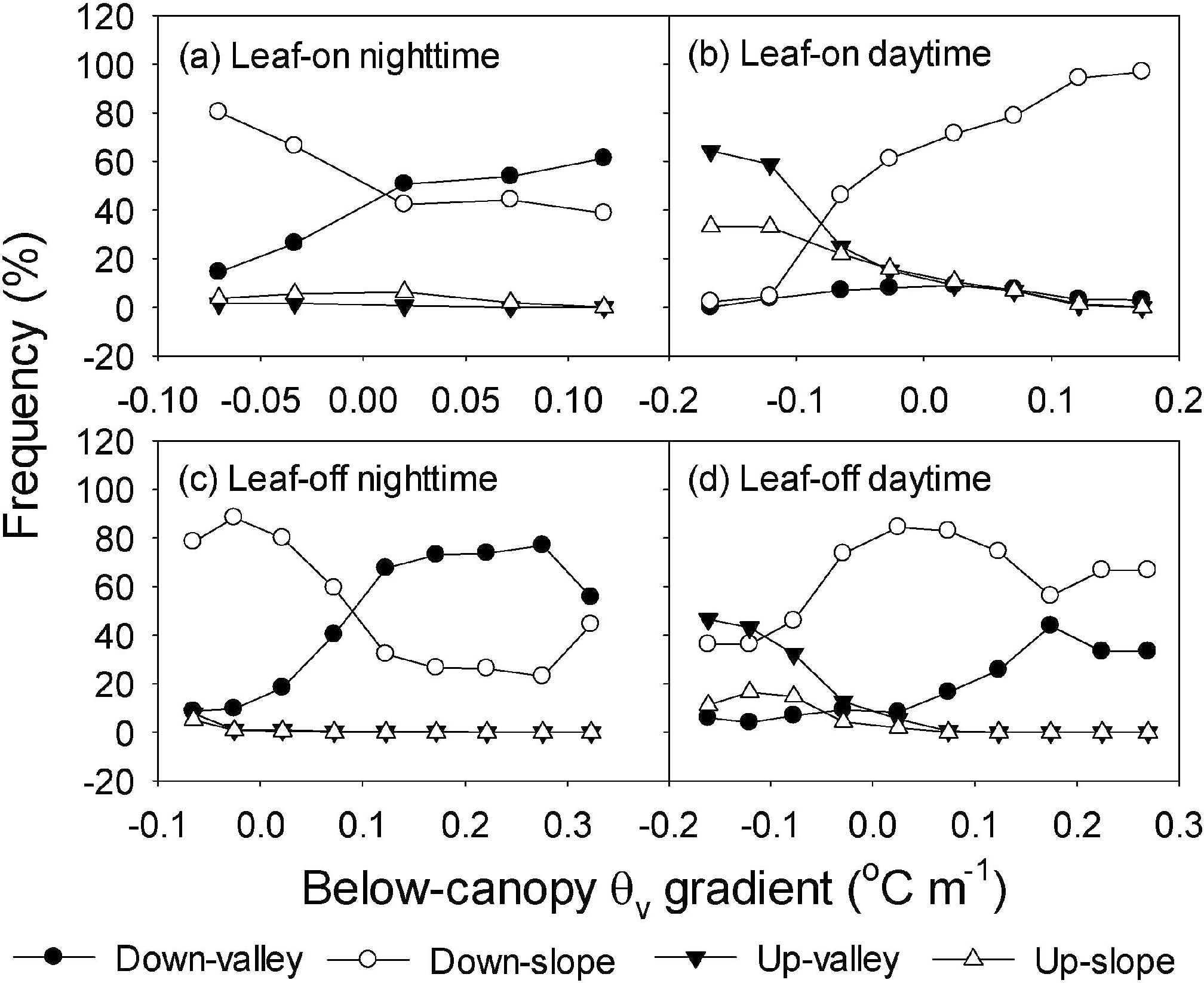
4.5.2. Below-Canopy


5. Conclusions
Acknowledgments
Author Contributions
Conflicts of Interest
References
- Baldocchi, D. Measuring fluxes of trace gases and energy between ecosystems and the atmosphere—The state and future of the eddy covariance method. Global. Change. Biol. 2014, 20, 3600–3609. [Google Scholar] [CrossRef]
- Aubinet, M.; Feigenwinter, C.; Heinesch, B.; Bernhofer, C.; Canepa, E.; Lindroth, A.; Montagnani, L.; Rebmann, C.; Sedlak, P.; van Gorsel, E. Direct advection measurements do not help to solve the night-time CO2 closure problem: Evidence from three different forests. Agric. For. Meteorol. 2010, 150, 655–664. [Google Scholar] [CrossRef]
- Feigenwinter, C.; Bernhofer, C.; Eichelmann, U.; Heinesch, B.; Hertel, M.; Janous, D.; Kolle, O.; Lagergren, F.; Lindroth, A.; Minerbi, S.; et al. Comparison of horizontal and vertical advective CO2 fluxes at three forest sites. Agric. For. Meteorol. 2008, 148, 12–24. [Google Scholar] [CrossRef]
- Lee, X. On micrometeorological observations of surface-air exchange over tall vegetation. Agric. For. Meteorol. 1998, 91, 39–49. [Google Scholar] [CrossRef]
- Sun, J.; Burns, S.P.; Delany, A.C.; Oncley, S.P.; Turnipseed, A.A.; Stephens, B.B.; Lenschow, D.H.; LeMone, M.A.; Monson, R.K.; Anderson, D.E. CO2 transport over complex terrain. Agric. For. Meteorol. 2007, 145, 1–21. [Google Scholar] [CrossRef]
- Van Gorsel, E.; Harman, I.N.; Finnigan, J.J.; Leuning, R. Decoupling of air flow above and in plant canopies and gravity waves affect micrometeorological estimates of net scalar exchange. Agric. For. Meteorol. 2011, 151, 927–933. [Google Scholar] [CrossRef]
- Staebler, R.M.; Fitzjarrald, D.R. Observing subcanopy CO2 advection. Agric. For. Meteorol. 2004, 122, 139–156. [Google Scholar] [CrossRef]
- Tóta, J.; Fitzjarrald, D.R.; Staebler, R.M.; Sakai, R.K.; Moraes, O.M.; Acevedo, O.C.; Wofsy, S.C.; Manzi, A.O. Amazon rain forest subcanopy flow and the carbon budget: Santarém lba-eco site. J. Geophys. Res. 2008. [Google Scholar] [CrossRef]
- Alekseychik, P.; Mammarella, I.; Launiainen, S.; Rannik, Ü.; Vesala, T. Evolution of the nocturnal decoupled layer in a pine forest canopy. Agric. For. Meteorol. 2013, 174–175, 15–27. [Google Scholar] [CrossRef]
- Froelich, N.; Schmid, H. Flow divergence and density flows above and below a deciduous forest: Part II. Below-canopy thermotopographic flows. Agric. For. Meteorol. 2006, 138, 29–43. [Google Scholar] [CrossRef]
- Novick, K.; Brantley, S.; Miniat, C.F.; Walker, J.; Vose, J.M. Inferring the contribution of advection to total ecosystem scalar fluxes over a tall forest in complex terrain. Agric. For. Meteorol. 2014, 185, 1–13. [Google Scholar] [CrossRef]
- Belcher, S.E.; Harman, I.N.; Finnigan, J.J. The wind in the willows: Flows in forest canopies in complex terrain. Annu. Rev. Fluid Mech. 2012, 44, 479–504. [Google Scholar] [CrossRef]
- Thomas, C.K.; Martin, J.G.; Law, B.E.; Davis, K. Toward biologically meaningful net carbon exchange estimates for tall, dense canopies: Multi-level eddy covariance observations and canopy coupling regimes in a mature douglas-fir forest in oregon. Agric. For. Meteorol. 2013, 173, 14–27. [Google Scholar] [CrossRef]
- Yi, C.; Monson, R.K.; Zhai, Z.; Anderson, D.E.; Lamb, B.; Allwine, G.; Turnipseed, A.A.; Burns, S.P. Modeling and measuring the nocturnal drainage flow in a high-elevation, subalpine forest with complex terrain. J. Geophys. Res. 2005. [Google Scholar] [CrossRef]
- Zardi, D.; Whiteman, C.D. Diurnal mountain wind systems. In Mountain Weather Research and Forecasting: Recent Progress and Current Challenges; Chow, F., de Wekker, S., Snyder, B., Eds.; Springer: Berlin, Germany, 2013; pp. 35–119. [Google Scholar]
- Grisogono, B.; Axelsen, S.L. A note on the pure katabatic wind maximum over gentle slopes. Bound.-Layer Meteorol. 2012, 145, 527–538. [Google Scholar] [CrossRef]
- Chen, H.; Yi, C. Optimal control of katabatic flows within canopies. Q. J. R. Meteor. Soc. 2012, 138, 1676–1680. [Google Scholar] [CrossRef]
- Burns, S.P.; Sun, J.; Lenschow, D.H.; Oncley, S.P.; Stephens, B.B.; Yi, C.; Anderson, D.E.; Hu, J.; Monson, R.K. Atmospheric stability effects on wind fields and scalar mixing within and just above a subalpine forest in sloping terrain. Bound.-Layer Meteorol. 2011, 138, 231–262. [Google Scholar] [CrossRef]
- Aubinet, M.; Berbigier, P.; Bernhofer, C.; Cescatti, A.; Feigenwinter, C.; Granier, A.; Grünwald, T.; Havrankova, K.; Heinesch, B.; Longdoz, B. Comparing CO2 storage and advection conditions at night at different carboeuroflux sites. Bound.-Layer Meteorol. 2005, 116, 63–93. [Google Scholar] [CrossRef]
- Whiteman, C.D.; Zhong, S. Downslope flows on a low-angle slope and their interactions with valley inversions. Part I: Observations. J. Appl. Meteorol. Climitol. 2008, 47, 2023–2038. [Google Scholar] [CrossRef]
- Trachte, K.; Nauss, T.; Bendix, J. The impact of different terrain configurations on the formation and dynamics of katabatic flows: Idealised case studies. Bound.-Layer Meteorol. 2010, 134, 307–325. [Google Scholar] [CrossRef]
- van Gorsel, E.; Christen, A.; Feigenwinter, C.; Parlow, E.; Vogt, R. Daytime turbulence statistics above a steep forested slope. Bound.-Layer Meteorol. 2003, 109, 311–329. [Google Scholar]
- Mahrt, L.; Richardson, S.; Seaman, N.; Stauffer, D. Non-stationary drainage flows and motions in the cold pool. Tellus A 2010, 62, 698–705. [Google Scholar]
- Belcher, S.; Finnigan, J.; Harman, I. Flows through forest canopies in complex terrain. Ecol. Appl. 2008, 18, 1436–1453. [Google Scholar] [CrossRef] [PubMed]
- Aubinet, M. Eddy covariance CO2 flux measurements in nocturnal conditions: An analysis of the problem. Ecol. Appl. 2008, 18, 1368–1378. [Google Scholar] [CrossRef] [PubMed]
- Kiefer, M.T.; Zhong, S. The effect of sidewall forest canopies on the formation of cold-air pools: A numerical study. J. Geophys. Res. 2013, 118, 5965–5978. [Google Scholar] [CrossRef]
- Froelich, N.; Grimmond, C.; Schmid, H. Nocturnal cooling below a forest canopy: Model and evaluation. Agric. For. Meteorol. 2011, 151, 957–968. [Google Scholar] [CrossRef]
- Mahrt, L. Stratified atmospheric boundary layers. Bound.-Layer Meteorol. 1999, 90, 375–396. [Google Scholar] [CrossRef]
- Pypker, T.; Unsworth, M.; Lamb, B.; Allwine, E.; Edburg, S.; Sulzman, E.; Mix, A.; Bond, B. Cold air drainage in a forested valley: Investigating the feasibility of monitoring ecosystem metabolism. Agric. For. Meteorol. 2007, 145, 149–166. [Google Scholar] [CrossRef]
- Tóta, J.; Roy Fitzjarrald, D.; da Silva Dias, M.A. Amazon rainforest exchange of carbon and subcanopy air flow: Manaus lba site—A complex terrain condition. Sci. World J. 2012. [Google Scholar] [CrossRef]
- Komatsu, H.; Yoshida, N.; Takizawa, H.; Kosaka, I.; Tantasirin, C.; Suzuki, M. Seasonal trend in the occurrence of nocturnal drainage flow on a forested slope under a tropical monsoon climate. Bound.-Layer Meteorol. 2003, 106, 573–592. [Google Scholar] [CrossRef]
- Pypker, T.G.; Unsworth, M.H.; Mix, A.C.; Rugh, W.; Ocheltree, T.; Alstad, K.; Bond, B.J. Using nocturnal cold air drainage flow to monitor ecosystem processes in complex terrain. Ecol. Appl. 2007, 17, 702–714. [Google Scholar] [CrossRef] [PubMed]
- Rotach, M.; Andretta, M.; Calanca, P.; Weigel, A.; Weiss, A. Boundary layer characteristics and turbulent exchange mechanisms in highly complex terrain. Acta Geophys. 2008, 56, 194–219. [Google Scholar] [CrossRef]
- Jiao, Z.; Wang, C.-K.; Wang, X.-C. Spatio-temporal variations of CO2 concentration within the canopy in a temperate deciduous forest, northeast China. Chin. J. Plant Ecol. 2011, 35, 512–522. [Google Scholar] [CrossRef]
- Mahrt, L. Momentum balance of gravity flows. J. Atmos. Sci. 1982, 39, 2701–2711. [Google Scholar] [CrossRef]
- Mahrt, L.; Vickers, D.; Nakamura, R.; Soler, M.R.; Sun, J.; Burns, S.; Lenschow, D.H. Shallow drainage flows. Bound.-Layer Meteorol. 2001, 101, 243–260. [Google Scholar] [CrossRef]
- Rotach, M.W.; Zardi, D. On the boundary-layer structure over highly complex terrain: Key findings from map. Q. J. R. Meteor. Soc. 2007, 133, 937–948. [Google Scholar] [CrossRef]
- Rebmann, C.; Zeri, M.; Lasslop, G.; Mund, M.; Kolle, O.F.; Schulze, E.-D.; Feigenwinter, C. Treatment and assessment of the CO2-exchange at a complex forest site in thuringia, germany. Agric. For. Meteorol. 2010, 150, 684–691. [Google Scholar] [CrossRef]
- Staebler, R.M.; Fitzjarrald, D.R. Measuring canopy structure and the kinematics of subcanopy flows in two forests. J. Appl. Meteorol. 2005, 44, 1161–1179. [Google Scholar] [CrossRef]
- Wang, C.; Han, Y.; Chen, J.; Wang, X.; Zhang, Q.; Bond-Lamberty, B. Seasonality of soil CO2 efflux in a temperate forest: Biophysical effects of snowpack and spring freeze–thaw cycles. Agric. For. Meteorol. 2013, 177, 83–92. [Google Scholar] [CrossRef]
- Wilczak, J.M.; Oncley, S.P.; Stage, S.A. Sonic anemometer tilt correction algorithms. Bound.-Layer Meteorol. 2001, 99, 127–150. [Google Scholar] [CrossRef]
- Yi, C. Momentum transfer within canopies. J. Appl. Meteorol. Climitol. 2008, 47, 262–275. [Google Scholar] [CrossRef]
- Mahrt, L.; Lee, X.; Black, A.; Neumann, H.; Staebler, R. Nocturnal mixing in a forest subcanopy. Agric. For. Meteorol. 2000, 101, 67–78. [Google Scholar] [CrossRef]
- Mahrt, L.; Vickers, D.; Sun, J.; Jensen, N.; Jørgensen, H.; Pardyjak, E.; Fernando, H. Determination of the surface drag coefficient. Bound.-Layer Meteorol. 2001, 99, 249–276. [Google Scholar] [CrossRef]
- Weber, R. Remarks on the definition and estimation of friction velocity. Bound.-Layer Meteorol. 1999, 93, 197–209. [Google Scholar] [CrossRef]
- Dupont, S.; Patton, E.G. Influence of stability and seasonal canopy changes on micrometeorology within and above an orchard canopy: The chats experiment. Agric. For. Meteorol. 2012, 157, 11–29. [Google Scholar] [CrossRef]
- Yao, Y.; Zhang, Y.; Liang, N.; Tan, Z.; Yu, G.; Sha, L.; Song, Q. Pooling of CO2 within a small valley in a tropical seasonal rain forest. J. Forest. Res. 2012, 17, 241–252. [Google Scholar] [CrossRef]
- Monti, P.; Fernando, H.; Princevac, M.; Chan, W.; Kowalewski, T.; Pardyjak, E. Observations of flow and turbulence in the nocturnal boundary layer over a slope. J. Atmos. Sci. 2002, 59, 2513–2534. [Google Scholar] [CrossRef]
- Burns, P.; Chemel, C. Evolution of cold-air-pooling processes in complex terrain. Bound.-Layer Meteorol. 2014, 150, 423–447. [Google Scholar] [CrossRef]
- Thomas, C.K. Variability of sub-canopy flow, temperature, and horizontal advection in moderately complex terrain. Bound.-Layer Meteorol. 2011, 139, 61–81. [Google Scholar] [CrossRef]
- Wu, J.; Guan, D.; Yuan, F.; Yang, H.; Wang, A.; Jin, C. Evolution of atmospheric carbon dioxide concentration at different temporal scales recorded in a tall forest. Atmos. Environ. 2012, 61, 9–14. [Google Scholar] [CrossRef]
- Aubinet, M.; Heinesch, B.; Yernaux, M. Horizontal and vertical CO2 advection in a sloping forest. Bound.-Layer Meteorol. 2003, 108, 397–417. [Google Scholar] [CrossRef]
- Kruijt, B.; Malhi, Y.; Lloyd, J.; Norbre, A.; Miranda, A.; Pereira, M.; Culf, A.; Grace, J. Turbulence statistics above and within two amazon rain forest canopies. Bound.-Layer Meteorol. 2000, 94, 297–331. [Google Scholar] [CrossRef]
- Sedlák, P.; Aubinet, M.; Heinesch, B.; Janouš, D.; Pavelka, M.; Potužníková, K.; Yernaux, M. Night-time airflow in a forest canopy near a mountain crest. Agric. For. Meteorol. 2010, 150, 736–744. [Google Scholar] [CrossRef]
- Bernardes, M.; Dias, N.L. The alignment of the mean wind and stress vectors in the unstable surface layer. Bound.-Layer Meteorol. 2010, 134, 41–59. [Google Scholar] [CrossRef]
- Su, H.-B.; Schmid, H.; Vogel, C.; Curtis, P. Effects of canopy morphology and thermal stability on mean flow and turbulence statistics observed inside a mixed hardwood forest. Agric. For. Meteorol. 2008, 148, 862–882. [Google Scholar] [CrossRef]
- Yi, C.; Anderson, D.E.; Turnipseed, A.A.; Burns, S.P.; Sparks, J.P.; Stannard, D.I.; Monson, R.K. The contribution of advective fluxes to net ecosystem exchange in a high-elevation, subalpine forest. Ecol. Appl. 2008, 18, 1379–1390. [Google Scholar] [CrossRef] [PubMed]
- Feigenwinter, C.; Montagnani, L.; Aubinet, M. Plot-scale vertical and horizontal transport of CO2 modified by a persistent slope wind system in and above an alpine forest. Agric. For. Meteorol. 2010, 150, 665–673. [Google Scholar] [CrossRef]
- Queck, R.; Bernhofer, C. Constructing wind profiles in forests from limited measurements of wind and vegetation structure. Agric. For. Meteorol. 2010, 150, 724–735. [Google Scholar] [CrossRef]
- Siebicke, L.; Hunner, M.; Foken, T. Aspects of CO2 advection measurements. Theor. Appl. Climatol. 2012, 109, 109–131. [Google Scholar] [CrossRef]
- Marcolla, B.; Cobbe, I.; Minerbi, S.; Montagnani, L.; Cescatti, A. Methods and uncertainties in the experimental assessment of horizontal advection. Agric. For. Meteorol. 2014, 198–199, 62–71. [Google Scholar] [CrossRef]
- Froelich, N.; Schmid, H.; Grimmond, C.; Su, H.-B.; Oliphant, A. Flow divergence and density flows above and below a deciduous forest: Part I. Non-zero mean vertical wind above canopy. Agric. For. Meteorol. 2005, 133, 140–152. [Google Scholar] [CrossRef]
- van Gorsel, E.; Delpierre, N.; Leuning, R.; Black, A.; Munger, J.W.; Wofsy, S.; Aubinet, M.; Feigenwinter, C.; Beringer, J.; Bonal, D. Estimating nocturnal ecosystem respiration from the vertical turbulent flux and change in storage of CO2. Agric. For. Meteorol. 2009, 149, 1919–1930. [Google Scholar]
- Gielen, B.; de Vos, B.; Campioli, M.; Neirynck, J.; Papale, D.; Verstraeten, A.; Ceulemans, R.; Janssens, I. Biometric and eddy covariance-based assessment of decadal carbon sequestration of a temperate scots pine forest. Agric. For. Meteorol. 2013, 174, 135–143. [Google Scholar] [CrossRef]
- Wu, J.; Larsen, K.; van der Linden, L.; Beier, C.; Pilegaard, K.; Ibrom, A. Synthesis on the carbon budget and cycling in a danish, temperate deciduous forest. Agric. For. Meteorol. 2013, 181, 94–107. [Google Scholar] [CrossRef]
© 2014 by the authors; licensee MDPI, Basel, Switzerland. This article is an open access article distributed under the terms and conditions of the Creative Commons Attribution license (http://creativecommons.org/licenses/by/4.0/).
Share and Cite
Wang, X.; Wang, C.; Li, Q. Wind Regimes above and below a Temperate Deciduous Forest Canopy in Complex Terrain: Interactions between Slope and Valley Winds. Atmosphere 2015, 6, 60-87. https://doi.org/10.3390/atmos6010060
Wang X, Wang C, Li Q. Wind Regimes above and below a Temperate Deciduous Forest Canopy in Complex Terrain: Interactions between Slope and Valley Winds. Atmosphere. 2015; 6(1):60-87. https://doi.org/10.3390/atmos6010060
Chicago/Turabian StyleWang, Xingchang, Chuankuan Wang, and Qinglin Li. 2015. "Wind Regimes above and below a Temperate Deciduous Forest Canopy in Complex Terrain: Interactions between Slope and Valley Winds" Atmosphere 6, no. 1: 60-87. https://doi.org/10.3390/atmos6010060
APA StyleWang, X., Wang, C., & Li, Q. (2015). Wind Regimes above and below a Temperate Deciduous Forest Canopy in Complex Terrain: Interactions between Slope and Valley Winds. Atmosphere, 6(1), 60-87. https://doi.org/10.3390/atmos6010060