Total Gaseous Mercury Concentration Measurements at Fort McMurray, Alberta, Canada

Abstract

Observations are described from total gaseous mercury (TGM) concentrations measured at the Wood Buffalo Environmental Association (WBEA) Fort McMurray—Patricia McInnes air quality monitoring station—from 21 October 2010 through 31 May 2013, inclusively. Fort McMurray is approximately 380 km north-northeast of Edmonton, Alberta, and approximately 30 km south of major Canadian oil sands developments. The average TGM concentration over the period of this study was 1.45 ± 0.18 ng∙m⁻³. Principal component analysis suggests that observed TGM concentrations are correlated with meteorological conditions including temperature, relative humidity, and solar radiation, and also ozone concentration. There is no significant correlation between ambient concentrations of TGM and anthropogenic pollutants, such as nitrogen oxides (NO_X) and sulphur dioxide (SO₂). Principal component analysis also shows that the highest TGM concentrations observed are a result of forest fire smoke near the monitoring station. Back trajectory analysis highlights the importance of long-range transport, indicating that unseasonably high TGM concentrations are generally associated with air from the southeast and west, while unseasonably low TGM concentrations are a result of arctic air moving over the monitoring station. In general, TGM concentration appears to be driven by diel and seasonal trends superimposed over a combination of long-range transport and regional surface-air flux of gaseous mercury.

1. Introduction

Total gaseous mercury (TGM) is ubiquitous in the atmosphere, persisting for up to 1.5 years, thus making mercury a pollutant of global concern due to potential long-range transport [1]. Mercury can exist in several forms in the atmosphere. The bulk (95–97%) of atmospheric mercury exists as gaseous elemental mercury (GEM), while the remainder consists of gaseous oxidized mercury (GOM) (also referred to as reactive gaseous mercury), and particulate bound mercury (PBM) [2,3,4]. TGM consists of both GEM and GOM, with typical ambient TGM concentrations in the range of 1.3–1.7 ng∙m⁻³ in the northern hemisphere [1,5,6]; within the province of Alberta in Canada, mean hourly TGM concentrations have been measured in the range of 1.36–1.65 ng∙m⁻³ [7,8]. Each form of mercury varies in its removal efficiencies via wet or dry deposition to surfaces where it can undergo further reactions, such as methylation to enhance toxicity and undergo bioaccumulation within the ecosystem [1,9]. A unique feature of mercury is its ability to re-emit following deposition, effectively increasing the atmospheric lifetime and global distribution of mercury. Thus, mercury can be found—to varying degrees—in all ecosystems, even in locations greatly removed from any major sources.

Atmospheric mercury has many anthropogenic sources including combustion of coal and other fuels (especially those with elevated mercury content) and mining activities; all of which are commonplace in and around the Canadian oil sands region of northern Alberta. Industries within the Regional Municipality of Wood Buffalo, which contains the urban center of Fort McMurray and the Canadian oil sands development, were reported as releasing 51 kg of industrial mercury emissions to the air in 2011, which is approximately 2% of industrial mercury air emissions for all of Canada in 2011 [10]. Likewise, industries in the region were also reported as releasing 6% and 8% of industrial NO_X and SO₂ emissions, respectively, for all of Canada [10]. In an attempt to better understand the effects of oil, gas, and bitumen extraction in the Canadian oil sands on atmospheric mercury concentrations, Environment Canada has operated—and continues to operate—a continuous ambient TGM analyzer at the Wood Buffalo Environmental Association (WBEA) Fort McMurray—Patricia McInnes air quality monitoring station (Patricia McInnes station herein). The analyzer measures ambient concentration of TGM in the community of Fort McMurray, Alberta, the urban hub of the Canadian oil sands region, approximately 30 km south of the nearest oil sands production facility (see Section 3.1 below for a site description and map of the area). No previous studies on ambient atmospheric mercury have been conducted in the Canadian oil sands region, despite the concentration of mining activity and other potential mercury sources present in this internationally scrutinized region subject to significant industrial and environmental regulations [11].

Several communities and groups are concerned that ecosystem-wide mercury concentrations are on the rise in the region, affecting local water and food sources, and exacerbated by the steady increase in industrial development in the area [12]. For example, Kelly et al. [13] measured greater mercury concentrations in water and snow near oil sands developments compared to locations further removed from developments. On the other hand, Wiklund et al. [14] note that, since the 1990s, increasing Canadian oil sands industrial development does not coincide with the decreasing trend in mercury concentrations in sediment cores downstream of the oil sands region. Thus, uncertainty remains regarding mercury sources, transport, and fate in the region, and it is important to consider the role of atmospheric mercury in these processes. In an effort to enhance pollutant monitoring over all aspects of the ecosystem in this region, the Canadian and Alberta governments initiated the Joint Canada-Alberta Implementation Plan for Oil Sands Monitoring [15]; the ambient atmospheric mercury measurement programme described here forms one piece of the air monitoring component of this plan. The objective of this study is to better understand the underlying factors driving atmospheric mercury concentrations in the oil sands region, which may, in turn, help to address knowledge gaps regarding the fate of mercury in the region.

2. Results and Discussion

2.1. General Trends and Statistics

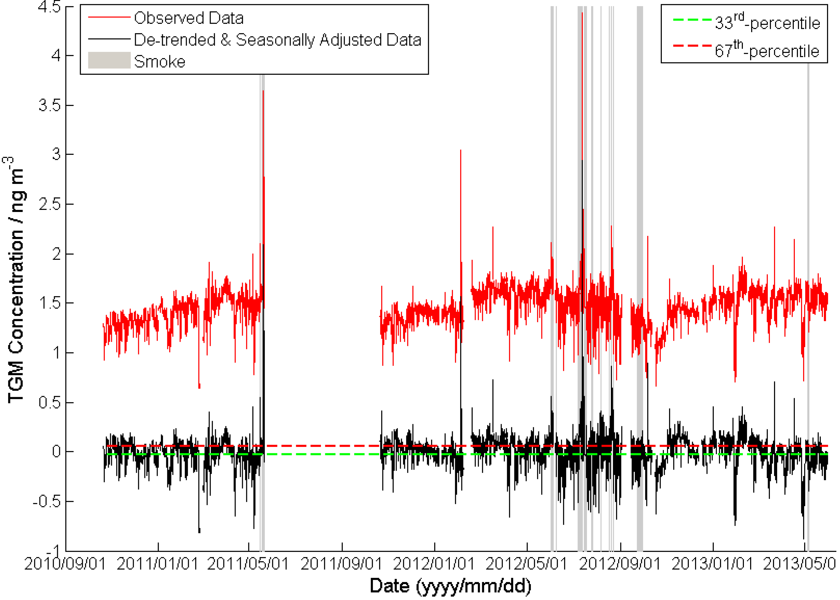
Figure 1 shows TGM concentrations measured at Patricia McInnes station from 21 October 2010 through 31 May 2013, inclusively. Summary statistics for these data are also listed in Table 1. The average TGM concentration at Patricia McInnes station over the course of this study was 1.45 ± 0.18 ng∙m⁻³, which is comparable to that measured at other stations in the province of Alberta (1.36–1.65 ng∙m⁻³ [7,8]). The gap in data from 21 May 2011 through 20 October 2011 was due to instrument contamination as noted in Section 3.3 below. There is a slight increasing trend in TGM concentrations measured at the Patricia McInnes station with a rate of 0.051 ± 0.003 ng∙m⁻³∙y⁻¹ over the range of the study period as determined with linear regression. Note that at approximately 2.5 years in length, this period of record is not sufficiently long to definitively regard this as a true long-term trend, and this trend reported may only represent a medium-term fluctuation within a different longer-term trend. As seen in Figure 1, there are several instances of elevated TGM concentrations. Most of these events coincide with forest fire smoke near the Patricia McInnes station as indicated by the shaded areas in Figure 1. Conversely, not all cases where forest fire smoke was present led to increased TGM concentrations. This may be due to the distance between the forest fire and the monitoring station, i.e., the age of the smoke. Data impacted by forest fire smoke is included in analyses described below except where noted. Figure 1 indicates that, aside from periods impacted by forest fire smoke, high TGM concentrations are generally observed over short time scales, whereas low TGM concentrations are generally observed over longer time scales. Table 1 shows the statistics for the data deemed to be measured during forest fire smoke events (N = 447) in relation to the data that was not impacted by forest fire smoke (N = 17,020).

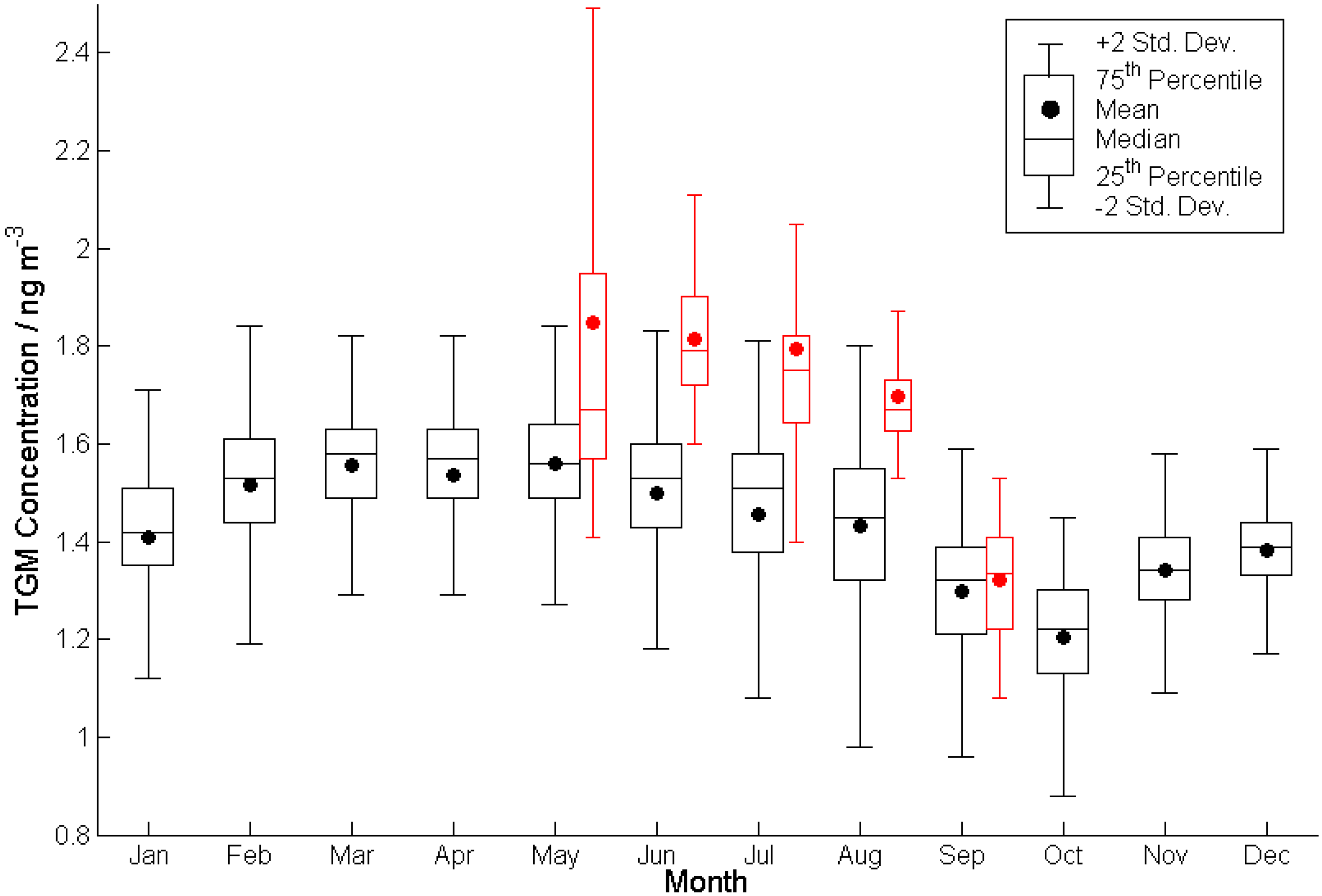
Figure 1 also shows ambient TGM concentrations to have a seasonal dependence. This is further illustrated in Figure 2, which shows the monthly averaged profile of TGM concentrations measured at Patricia McInnes station. Figure 2 shows a maximum in the spring and a minimum in the fall for data not impacted by forest fire smoke (black data), a pattern that has been observed in other similar locations and linked to meteorological cycles [8,16,17]. Forest fire smoke was only present during the months of May through September, inclusively, as shown in Figure 2 (red data). In general, mean monthly TGM is significantly higher in these months (p < 0.0001; d.f. ≥ 654) when forest fire smoke was present than when it was not, with the exception of September (p = 0.16; d.f. = 423), according to t-tests of monthly mean values.

Figure 1. Time series of hourly total gaseous mercury (TGM) concentrations at Patricia McInnes station. Grey shaded areas indicate when forest fire smoke was in the vicinity of the monitoring station. The de-trended/seasonally adjusted TGM time series is shown for reference. As described in the text, TGM concentration data was categorized as “high”, “average”, or “low”, with divisions at the 33rd- and 67th-percentiles in de-trended/seasonally adjusted TGM concentration.

Figure 1. Time series of hourly total gaseous mercury (TGM) concentrations at Patricia McInnes station. Grey shaded areas indicate when forest fire smoke was in the vicinity of the monitoring station. The de-trended/seasonally adjusted TGM time series is shown for reference. As described in the text, TGM concentration data was categorized as “high”, “average”, or “low”, with divisions at the 33rd- and 67th-percentiles in de-trended/seasonally adjusted TGM concentration.

Table 1. Summary statistics for Patricia McInnes station hourly TGM concentration data.

Dataset	Date Range	N	Mean (ng∙m−3)	Median (ng∙m−3)	Standard Deviation (ng∙m−3)	Minimum (ng∙m−3)	Maximum (ng∙m−3)
All data	21 October 2010–31 May 2013	17467	1.45	1.46	0.18	0.64	4.43
Excluding smoke		17020	1.45	1.46	0.17	0.64	3.05
Only smoke		447	1.73	1.69	0.34	1.08	4.43

Table 1. Summary statistics for Patricia McInnes station hourly TGM concentration data.

Dataset	Date Range	N	Mean (ng∙m−3)	Median (ng∙m−3)	Standard Deviation (ng∙m−3)	Minimum (ng∙m−3)	Maximum (ng∙m−3)
All data	21 October 2010–31 May 2013	17467	1.45	1.46	0.18	0.64	4.43
Excluding smoke		17020	1.45	1.46	0.17	0.64	3.05
Only smoke		447	1.73	1.69	0.34	1.08	4.43

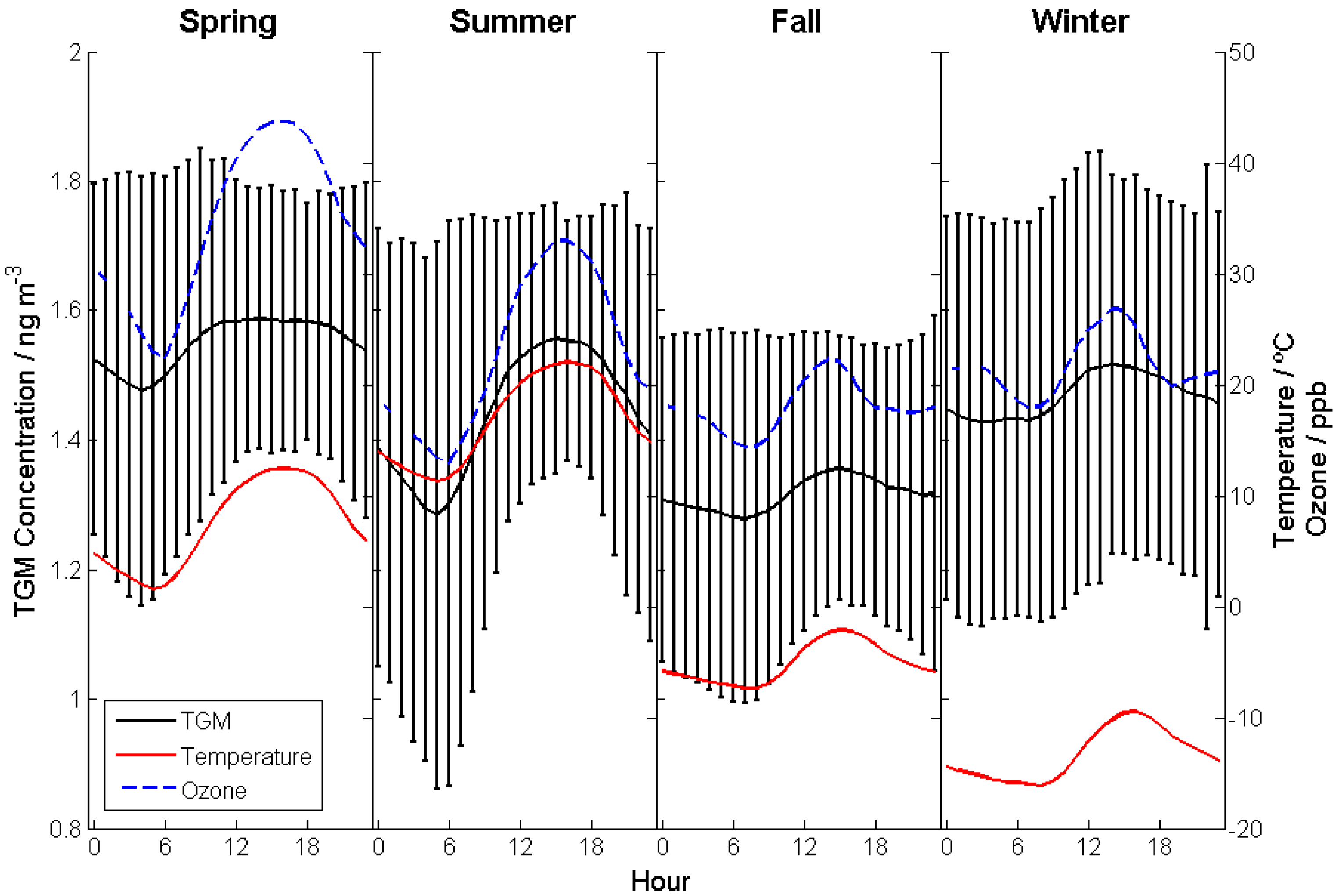
Figure 3 shows the diel profile of mean TGM concentrations for each season (spring: 21 March–20 June; summer: 21 June–20 September; fall: 21 September–20 December; winter: 21 December–20 March). As observed in other studies [16,18], minimum and maximum TGM concentrations are observed in the morning and in the afternoon-evening, respectively. Seasonal diel profiles of TGM concentrations qualitatively resemble those of the mean temperatures and ozone concentrations at Patricia McInnes (Figure 3) and highlight the relationship between these variables under average conditions. This relationship is also identified in the principal component analyses described in Section 2.2.

Figure 2. Monthly averaged TGM concentrations measured at Patricia McInnes station. Red data are impacted by forest fire smoke, whereas black data are not.

Figure 2. Monthly averaged TGM concentrations measured at Patricia McInnes station. Red data are impacted by forest fire smoke, whereas black data are not.

Figure 3. Seasonal diel profiles of mean TGM concentrations at Patricia McInnes station after removing data impacted by forest fire smoke. Seasonal diel profiles of mean temperatures and ozone concentrations at Patricia McInnes are also shown for reference Vertical bars indicate ± 2 standard deviations of TGM concentration data at each hour.

Figure 3. Seasonal diel profiles of mean TGM concentrations at Patricia McInnes station after removing data impacted by forest fire smoke. Seasonal diel profiles of mean temperatures and ozone concentrations at Patricia McInnes are also shown for reference Vertical bars indicate ± 2 standard deviations of TGM concentration data at each hour.

2.2. Principal Component Analysis

In addition to TGM concentration measurements, other air quality and meteorological measurements were considered, as described in Section 3.2. Air quality parameters include nitrous oxide (NO), nitrogen dioxide (NO₂), oxides of nitrogen (NO_X), ozone (O₃), fine particulate matter (PM_2.5), sulphur dioxide (SO₂), total hydrocarbon (THC), total reduced sulphur (TRS), ammonia (NH₃), and carbon monoxide (CO). Meteorological parameters include temperature (T), relative humidity (RH), wind speed and direction, solar radiation, and snow depth. Principal component analysis (PCA) was performed to identify correlations between parameters and serves as a means for reducing the number of parameters in the dataset into a handful of important factors. PCA was similarly applied in previous work where TGM concentrations were measured alongside a variety of ancillary variables to quantify relationships within the dataset and identify common factors that may influence TGM concentrations [19]. Three data subsets were established in order to better understand the factors affecting TGM and other air quality and meteorological parameters. The data subsets are grouped by rank according to “high”, “average”, and “low” TGM concentrations (i.e., three bins divided at the 33rd- and 67th-percentiles). In order to avoid biasing data subsets with predominately spring values in the “high” subset or fall values in the “low” subset, for example, the TGM concentration data was de-trended and seasonally adjusted only to categorize any given TGM concentration as “high”, “average”, or “low”, but the original TGM concentration values were used as input for PCA. De-trending and seasonal adjustment was carried out with additive decomposition with a linear trend component and 4th-order polynomial fit to monthly averaged data (similar to that shown in Figure 2) as a seasonal filter [20,21]. The de-trended and seasonally adjusted time series is shown in Figure 1 for reference. PCA results for each data subset, “high”, “average”, and “low” TGM concentrations, are shown in Table 2, Table 3 and Table 4, respectively. For comparison, PCA results for the full, combined dataset are shown in Table 5. These tables show the rotated factor loadings, the amount of variability explained by each factor and the eigenvalues. Only factors with eigenvalues greater than 1 are deemed significant and are interpreted below [22]. Parameters are an important contribution to a given factor when the absolute value of the corresponding rotated factor loading is ≥ 0.5 (bold values in Table 2 through Table 4) [22]. The meaning of each factor was inferred based on the groupings of parameters that load heaviest on that factor (e.g., NO_X is interpreted as anthropogenic combustion processes, and PM_2.5, CO, and NH₃ together are interpreted as forest fire smoke).

Table 2. Principal component analysis (PCA) rotated factor loadings for the highest 1/3rd of de-trended/seasonally adjusted TGM concentrations (i.e., “high” TGM concentrations). Factor loadings with an absolute value greater than or equal to 0.5 are bolded. The shaded row highlights TGM loadings on each factor.

Parameter	Combustion Processes	Diel Trending	Forest Fire Smoke	Snow Depth	Industrial Sulphur
NO	0.93	0.04	0.03	0.06	0.01
NO2	0.86	0.28	0.06	0.16	0.14
NOX	0.96	0.17	0.05	0.12	0.08
THC	0.60	0.04	0.25	−0.45	0.32
O3	−0.55	−0.70	0.01	0.07	−0.10
Temperature	−0.23	−0.68	0.19	−0.48	0.01
RH	0.14	0.86	0	0.12	0.11
Solar Radiation	−0.03	−0.78	−0.03	−0.12	0.09
TGM	−0.05	−0.49	0.59	0.28	0.17
PM2.5	0.06	−0.05	0.87	−0.11	0.17
NH3	0.02	0.04	0.74	0.01	−0.06
CO	0.11	0	0.79	−0.10	−0.03
Snow Depth	0.22	0.35	−0.01	0.81	0.08
SO2	0.05	−0.05	−0.06	0.22	0.83
TRS	0.25	0.10	0.19	−0.35	0.70
Variability (%)	22.7	18.6	16.1	9.5	9.4
Cumulative Variability (%)	22.7	41.3	57.5	67.0	76.4
Eigenvalues	4.62	2.99	1.60	1.13	1.11

Table 2. Principal component analysis (PCA) rotated factor loadings for the highest 1/3rd of de-trended/seasonally adjusted TGM concentrations (i.e., “high” TGM concentrations). Factor loadings with an absolute value greater than or equal to 0.5 are bolded. The shaded row highlights TGM loadings on each factor.

Parameter	Combustion Processes	Diel Trending	Forest Fire Smoke	Snow Depth	Industrial Sulphur
NO	0.93	0.04	0.03	0.06	0.01
NO2	0.86	0.28	0.06	0.16	0.14
NOX	0.96	0.17	0.05	0.12	0.08
THC	0.60	0.04	0.25	−0.45	0.32
O3	−0.55	−0.70	0.01	0.07	−0.10
Temperature	−0.23	−0.68	0.19	−0.48	0.01
RH	0.14	0.86	0	0.12	0.11
Solar Radiation	−0.03	−0.78	−0.03	−0.12	0.09
TGM	−0.05	−0.49	0.59	0.28	0.17
PM2.5	0.06	−0.05	0.87	−0.11	0.17
NH3	0.02	0.04	0.74	0.01	−0.06
CO	0.11	0	0.79	−0.10	−0.03
Snow Depth	0.22	0.35	−0.01	0.81	0.08
SO2	0.05	−0.05	−0.06	0.22	0.83
TRS	0.25	0.10	0.19	−0.35	0.70
Variability (%)	22.7	18.6	16.1	9.5	9.4
Cumulative Variability (%)	22.7	41.3	57.5	67.0	76.4
Eigenvalues	4.62	2.99	1.60	1.13	1.11

Table 3. PCA rotated factor loadings for the middle 1/3rd of de-trended/seasonally adjusted TGM concentrations (i.e., “average” TGM concentrations). Factor loadings with an absolute value greater than or equal to 0.5 are bolded. The shaded row highlights TGM loadings on each factor.

Parameter	Combustion Processes & NH3	Diel Trending	Industrial Sulphur & PM	Temperature & Snow Depth	CO
NO	0.89	0.07	0.14	0.07	0.10
NO2	0.70	0.29	0.36	0.30	0.20
NOX	0.87	0.20	0.28	0.20	0.17
NH3	0.64	−0.11	−0.25	−0.11	−0.35
THC	0.49	0.39	0.42	−0.30	0.07
TGM	−0.06	−0.76	0.05	0.28	0.05
O3	−0.48	−0.70	−0.27	−0.07	−0.18
Temperature	−0.19	−0.60	0	−0.63	0.18
RH	0.09	0.81	0.03	0.20	−0.01
Solar Radiation	0.02	−0.70	0.05	−0.18	0.01
PM2.5	0.29	−0.13	0.55	0.02	0.34
SO2	−0.03	−0.15	0.71	0.27	−0.19
TRS	0.19	0.17	0.69	−0.16	−0.07
Snow Depth	0.11	0.08	0.04	0.91	0.09
CO	0.09	−0.04	−0.10	0.01	0.86
Variability (%)	20.8	19.5	12.3	11.5	7.8
Cumulative Variability (%)	20.8	40.2	52.5	64.0	71.8
Eigenvalues	4.80	2.16	1.52	1.23	1.06

Table 3. PCA rotated factor loadings for the middle 1/3rd of de-trended/seasonally adjusted TGM concentrations (i.e., “average” TGM concentrations). Factor loadings with an absolute value greater than or equal to 0.5 are bolded. The shaded row highlights TGM loadings on each factor.

Parameter	Combustion Processes & NH3	Diel Trending	Industrial Sulphur & PM	Temperature & Snow Depth	CO
NO	0.89	0.07	0.14	0.07	0.10
NO2	0.70	0.29	0.36	0.30	0.20
NOX	0.87	0.20	0.28	0.20	0.17
NH3	0.64	−0.11	−0.25	−0.11	−0.35
THC	0.49	0.39	0.42	−0.30	0.07
TGM	−0.06	−0.76	0.05	0.28	0.05
O3	−0.48	−0.70	−0.27	−0.07	−0.18
Temperature	−0.19	−0.60	0	−0.63	0.18
RH	0.09	0.81	0.03	0.20	−0.01
Solar Radiation	0.02	−0.70	0.05	−0.18	0.01
PM2.5	0.29	−0.13	0.55	0.02	0.34
SO2	−0.03	−0.15	0.71	0.27	−0.19
TRS	0.19	0.17	0.69	−0.16	−0.07
Snow Depth	0.11	0.08	0.04	0.91	0.09
CO	0.09	−0.04	−0.10	0.01	0.86
Variability (%)	20.8	19.5	12.3	11.5	7.8
Cumulative Variability (%)	20.8	40.2	52.5	64.0	71.8
Eigenvalues	4.80	2.16	1.52	1.23	1.06

Table 4. PCA rotated factor loadings for lowest 1/3rd of de-trended/seasonally adjusted TGM concentrations (i.e., “low” TGM concentrations). Factor loadings with an absolute value greater than or equal to 0.5 are bolded. The shaded row highlights TGM loadings on each factor.

Parameter	Combustion Processes	Diel Trending	Temperature & Snow Depth	Industrial Sulphur & NH3
NO	0.85	0.06	0.16	0.08
NO2	0.74	0.17	0.51	−0.07
NOX	0.88	0.12	0.34	0.01
PM2.5	0.59	−0.12	0.07	−0.31
THC	0.68	0.42	−0.16	−0.1
O3	−0.54	−0.71	−0.06	0
TGM	−0.02	−0.72	0.05	0.02
RH	0.03	0.83	−0.03	0.02
Solar Radiation	0.05	−0.64	−0.34	−0.02
Temperature	−0.14	−0.26	−0.87	0.03
Snow Depth	0.07	−0.14	0.9	−0.06
SO2	0.16	−0.17	0.28	−0.61
TRS	0.49	0.11	−0.07	−0.51
NH3	0.21	−0.07	0.08	0.61
CO	0.41	−0.10	−0.10	0.20
Variability (%)	24.5	16.7	14.9	7.8
Cumulative Variability (%)	24.5	41.2	56.1	63.9
Eigenvalues	4.61	2.14	1.74	1.10

Table 4. PCA rotated factor loadings for lowest 1/3rd of de-trended/seasonally adjusted TGM concentrations (i.e., “low” TGM concentrations). Factor loadings with an absolute value greater than or equal to 0.5 are bolded. The shaded row highlights TGM loadings on each factor.

Parameter	Combustion Processes	Diel Trending	Temperature & Snow Depth	Industrial Sulphur & NH3
NO	0.85	0.06	0.16	0.08
NO2	0.74	0.17	0.51	−0.07
NOX	0.88	0.12	0.34	0.01
PM2.5	0.59	−0.12	0.07	−0.31
THC	0.68	0.42	−0.16	−0.1
O3	−0.54	−0.71	−0.06	0
TGM	−0.02	−0.72	0.05	0.02
RH	0.03	0.83	−0.03	0.02
Solar Radiation	0.05	−0.64	−0.34	−0.02
Temperature	−0.14	−0.26	−0.87	0.03
Snow Depth	0.07	−0.14	0.9	−0.06
SO2	0.16	−0.17	0.28	−0.61
TRS	0.49	0.11	−0.07	−0.51
NH3	0.21	−0.07	0.08	0.61
CO	0.41	−0.10	−0.10	0.20
Variability (%)	24.5	16.7	14.9	7.8
Cumulative Variability (%)	24.5	41.2	56.1	63.9
Eigenvalues	4.61	2.14	1.74	1.10

Focusing on the factors in relation to TGM, Table 2 correlates “high” TGM concentrations with parameters that are associated with forest fire smoke, namely: PM_2.5, CO, and NH₃ [23]. In other words, and not surprisingly, many of the high values in TGM are often a result of forest fire smoke impinging on the station. The next important factor for TGM during “high” TGM concentration observations relates to diel trending that strongly links ozone, temperature, RH, and solar radiation. TGM also shows minimal loading on the factor attributed to snow depth for the “high” TGM concentration data subset, which is not surprising given the strong association between “high” TGM concentration observations and forest fire smoke during the summer when there is no snow cover. PCA results for the “average” TGM concentration data subset (Table 3) show a shift of TGM correlation to the diel trending factor shared with ozone, temperature, RH, and solar radiation. The next important factor for TGM during “average” TGM concentration observations relates to temperature and snow depth. Similarly, PCA results for the “low” TGM concentration data subset (Table 4) also correlate TGM with diel trending ozone, RH, and solar radiation (but not temperature). Note that, in general, temperature is not as strongly associated with diel trending factors in all the PCA result tables, likely due to the wide variability of temperature in this region. Interestingly, for “average” and “low” TGM concentration subsets, TGM is effectively unrelated to pollutants mainly associated with local anthropogenic sources (i.e., NO, NO₂, NO_X, SO₂, TRS). Likewise, “high” TGM concentration data is very minimally, and essentially insignificantly, associated with SO₂ and TRS. Considering the PCA results from the complete dataset in Table 5, the overall ranking of importance for factors driving TGM variability is: diel trending > forest fire smoke > temperature and snow depth > industrial sulphur > combustion processes. 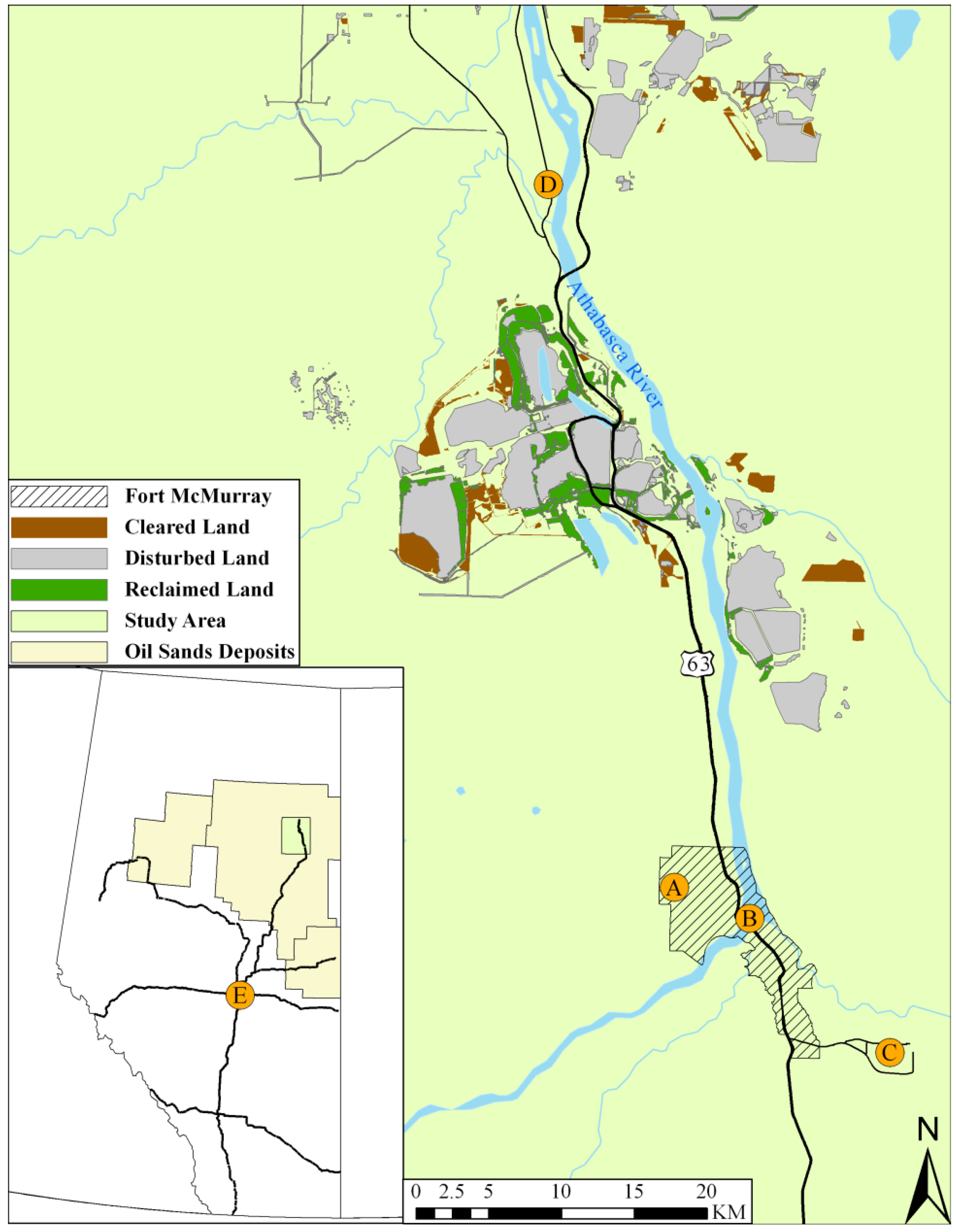Thus, Table 5 further indicates the lack of association between industrial pollutants and TGM. This is despite the fact that the station is within an urban area and near the industrialized center of the Canadian oil sands region.

Table 5. PCA rotated factor loadings for the full, combined dataset. Factor loadings with an absolute value greater than or equal to 0.5 are bolded. The shaded row highlights TGM loadings on each factor.

Parameter	Combustion Processes	Diel Trending	Forest Fire Smoke	Temperature & Snow Depth	Industrial Sulphur
NO	0.92	0	0.07	0.06	0.01
NO2	0.83	0.20	0.09	0.29	0.17
NOX	0.96	0.10	0.08	0.19	0.09
THC	0.62	0.27	0.15	−0.39	0.28
O3	−0.56	−0.70	−0.01	0.01	−0.08
TGM	−0.12	−0.65	0.37	0.24	0.14
RH	0.10	0.84	0.02	0.12	0.07
Solar Radiation	0.01	−0.73	−0.07	−0.25	0.03
Temperature	−0.26	−0.54	0.15	−0.64	−0.01
PM2.5	0.08	−0.07	0.82	−0.06	−0.31
CO	0.12	−0.06	0.71	−0.03	−0.06
NH3	0.03	0.04	0.73	0	−0.04
Snow Depth	0.17	−0.11	0	0.89	0.06
SO2	0.04	−0.11	−0.06	0.24	0.80
TRS	0.27	0.11	0.16	−0.21	0.73
Variability (%)	22.5	17.4	13.0	11.4	9.2
Cumulative Variability (%)	22.5	39.9	52.9	64.3	73.5
Eigenvalues	4.53	2.48	1.50	1.42	1.10

Table 5. PCA rotated factor loadings for the full, combined dataset. Factor loadings with an absolute value greater than or equal to 0.5 are bolded. The shaded row highlights TGM loadings on each factor.

Parameter	Combustion Processes	Diel Trending	Forest Fire Smoke	Temperature & Snow Depth	Industrial Sulphur
NO	0.92	0	0.07	0.06	0.01
NO2	0.83	0.20	0.09	0.29	0.17
NOX	0.96	0.10	0.08	0.19	0.09
THC	0.62	0.27	0.15	−0.39	0.28
O3	−0.56	−0.70	−0.01	0.01	−0.08
TGM	−0.12	−0.65	0.37	0.24	0.14
RH	0.10	0.84	0.02	0.12	0.07
Solar Radiation	0.01	−0.73	−0.07	−0.25	0.03
Temperature	−0.26	−0.54	0.15	−0.64	−0.01
PM2.5	0.08	−0.07	0.82	−0.06	−0.31
CO	0.12	−0.06	0.71	−0.03	−0.06
NH3	0.03	0.04	0.73	0	−0.04
Snow Depth	0.17	−0.11	0	0.89	0.06
SO2	0.04	−0.11	−0.06	0.24	0.80
TRS	0.27	0.11	0.16	−0.21	0.73
Variability (%)	22.5	17.4	13.0	11.4	9.2
Cumulative Variability (%)	22.5	39.9	52.9	64.3	73.5
Eigenvalues	4.53	2.48	1.50	1.42	1.10

2.3. Directional and Back Trajectory Analyses

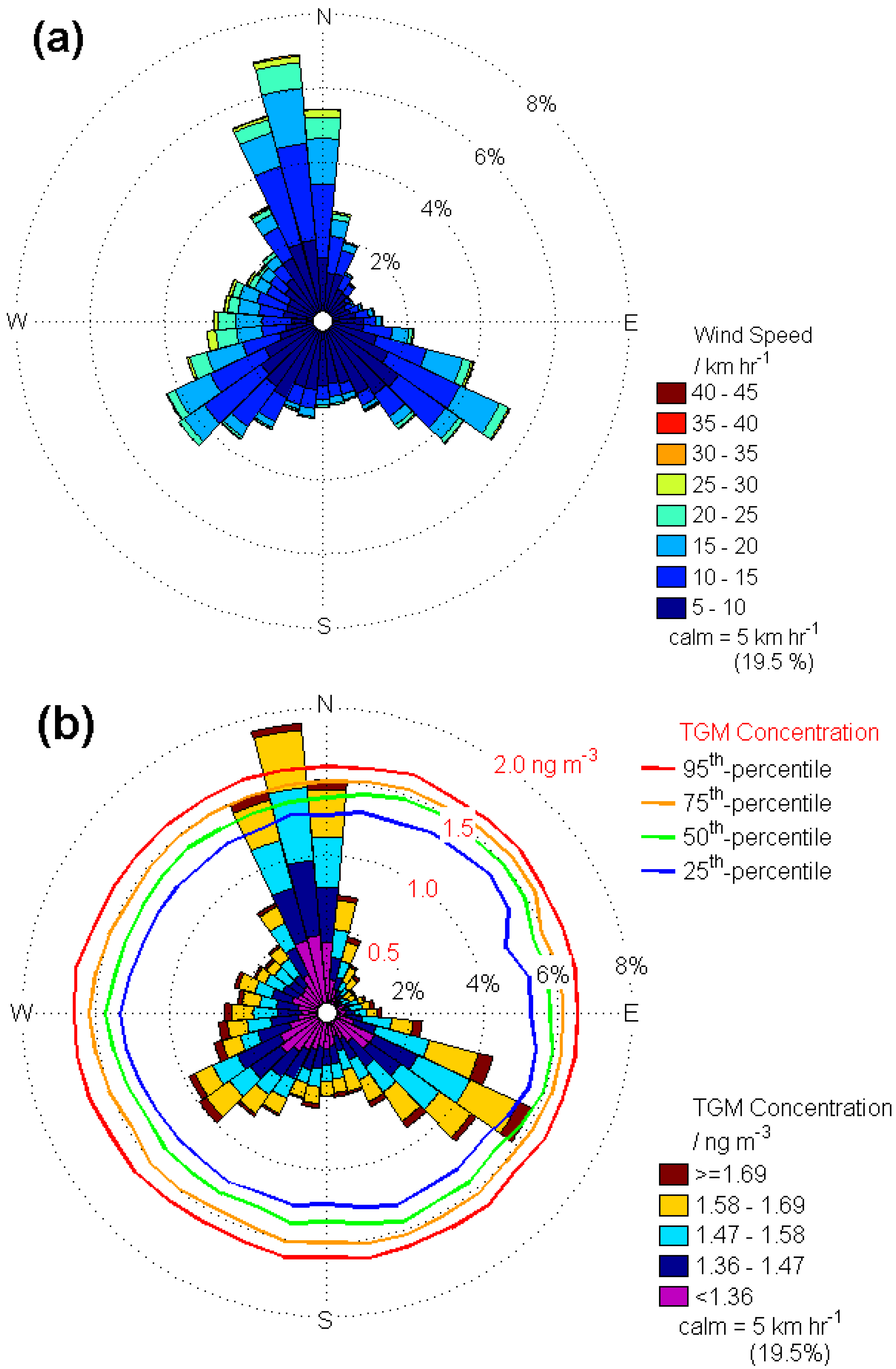
Although the PCA results suggest a lack of localized industrial source influences on TGM concentrations, the directionality of TGM concentrations was explored and is plotted as a pollutant rose alongside a wind rose in Figure 4. Note that the pollution rose in Figure 4b excludes both data observed in calm wind conditions (where wind speed < 5 km∙h⁻¹) and data impacted by forest fire smoke. Although the pollution rose, plotted as bars on the black axis in Figure 4b, at first appears to suggest possible point-sources to the north-northwest (i.e., oil sands development) and southeast (i.e., urban sources within Fort McMurray), a comparison to the wind rose (Figure 4a) indicates similar north-northwest and southeast dominant wind direction. The predominant winds at the station follow river valleys from the north-northwest and the southeast, hence TGM is simply observed from wherever the wind originates with minimal increased weighting toward any direction of a point-source. This is further illustrated with the directionally dependent TGM concentration percentiles, plotted as lines on the red axis in Figure 4b, which do not indicate any significant directional dependence to TGM concentrations. Thus, both the PCA results and Figure 4 suggest a limited role of local point-source influences on ambient TGM concentrations. These results suggest that the TGM observed at Patricia McInnes is predominately due to broad area sources (i.e., surface flux) and long-range transport.

Figure 4. (a) Wind rose and (b) TGM concentration rose for Patricia McInnes station. Data corresponding to calm winds (wind speed < 5 km∙h⁻¹) are not shown here. The TGM rose excludes data impacted by forest fire smoke. Frequency of concentration observations are plotted on the black scale and percentiles in TGM concentrations are plotted on the red radial axis in panel (b).

Figure 4. (a) Wind rose and (b) TGM concentration rose for Patricia McInnes station. Data corresponding to calm winds (wind speed < 5 km∙h⁻¹) are not shown here. The TGM rose excludes data impacted by forest fire smoke. Frequency of concentration observations are plotted on the black scale and percentiles in TGM concentrations are plotted on the red radial axis in panel (b).

Since the PCA results and Figure 4 suggest that local conditions were not sufficient to explain all observations of TGM concentrations, the role of long-range transport was assessed for the observations at Patricia McInnes. To investigate the role of long-range transport, back trajectories were calculated with the Hybrid Single Particle Lagrangian Integrated Trajectory (HYSPLIT) model [24,25]. 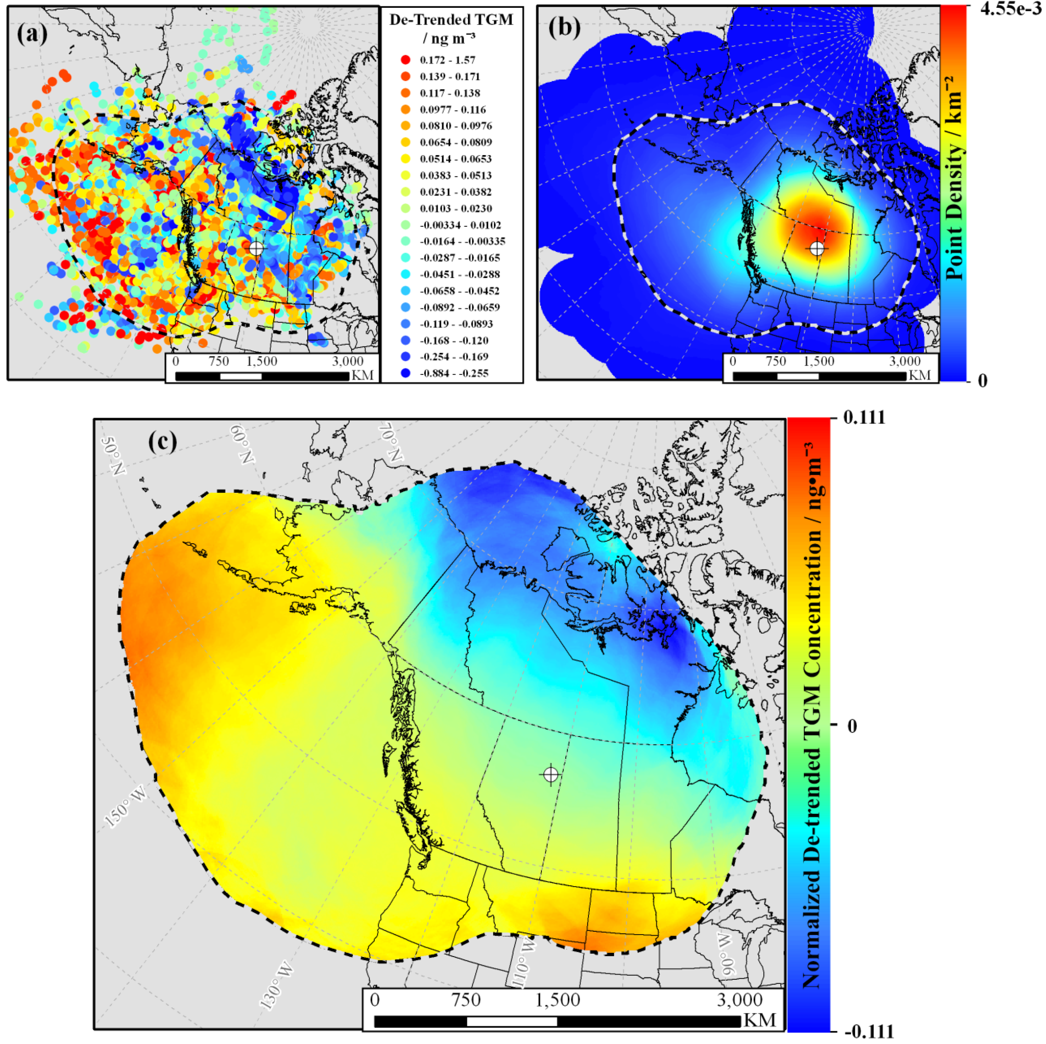Back trajectory analysis has been identified as an important tool for assessing the history of air masses influencing concentration measurements of atmospheric species [26]. The 72-hour HYSPLIT back trajectories from Patricia McInnes station were obtained for all observations of hourly TGM concentrations. Data observed with forest fire smoke were excluded from this analysis. The coordinates of the starting point of each back trajectory were plotted in ArcMap10 as points in Figure 5a where the colour of each point represents the de-trended/seasonally adjusted TGM concentration observed with each back trajectory (as defined in Section 2.2 and Figure 1). De-trended/seasonally adjusted TGM concentrations were used rather than actual TGM concentrations to gain insight into which regions were most frequently associated with unseasonably high or low TGM concentrations for any given time of year, rather than the times of year when higher or lower TGM concentrations are expected (as shown in Figure 2). Due to the presence of many overlapping points, Figure 5b shows the same back trajectory starting points, but illustrated as point density (see Section 3.5 for further details on point density mapping). Figure 5b indicates that most 72-hour back trajectory starting points were located in northern Alberta, northern Saskatchewan, northern British Columbia, and southern Northwest Territories where the highest point density is mapped in red. Only a limited number of back trajectories started outside western Canada, where the lowest point density is mapped in blue in Figure 5b; grey regions in Figure 5b indicate where no back trajectory starting points exist within a 700 km radius. Subsequently, a boundary condition to this back trajectory analysis was set to exclude regions with less than 1% of the total point density (i.e., fewer than 170 back trajectory starting points within a 700 km radius neighborhood), represented as the dashed lines in Figure 5a–c. Regions outside this dashed line were deemed to have an insufficient number of back trajectory starting points to draw any useful conclusions. Finally, Figure 5c shows the point density of back trajectory starting points weighted with de-trended/seasonally adjusted TGM concentrations and normalized by the point density shown in Figure 5b, resulting in a normalized de-trended/seasonally adjusted TGM concentration map (see Section 3.5). Red and blue areas in Figure 5c correspond to areas leading to the highest and lowest normalized de-trended/seasonally adjusted TGM concentration observations, respectively. The grey areas in Figure 5c are outside the boundary limits of the analysis due to an insufficient number of back trajectory starting points.

Figure 5c shows that the lowest normalized de-trended/seasonally adjusted TGM concentration observations primarily arrive via arctic regions of northern Canada. This region has minimal land disturbance or industry, so lower TGM concentration observations from air passing through this region are not surprising. Note that this back trajectory analysis cannot clearly distinguish between lower TGM concentrations originating from arctic regions as a result of arctic atmospheric mercury depletion events (AMDEs) [1,3,5,27,28,29,30,31] as opposed to as a result of generally cleaner air (i.e., air with lower TGM concentrations). However, given that during the study period, arctic air parcels are often associated with unseasonably lower TGM concentrations, this possibility is explored further in Section 2.4 below.

Figure 5. HYSPLIT 72-hour back trajectory analysis. Panel (a) shows all back trajectory starting points colour-coded to the corresponding de-trended/seasonally adjusted TGM concentrations; panel (b) shows the point density of back trajectory starting points; panel (c) shows the normalized de-trended/seasonally adjusted TGM concentrations as described in the text. Dashed lines indicate the boundary limits of the analysis as described in the text; grey areas contained insufficient or no back trajectory starting points. Fort McMurray is indicated in northern Alberta with the cross-hair symbol. Data observed with forest fire smoke were excluded from this analysis.

Figure 5. HYSPLIT 72-hour back trajectory analysis. Panel (a) shows all back trajectory starting points colour-coded to the corresponding de-trended/seasonally adjusted TGM concentrations; panel (b) shows the point density of back trajectory starting points; panel (c) shows the normalized de-trended/seasonally adjusted TGM concentrations as described in the text. Dashed lines indicate the boundary limits of the analysis as described in the text; grey areas contained insufficient or no back trajectory starting points. Fort McMurray is indicated in northern Alberta with the cross-hair symbol. Data observed with forest fire smoke were excluded from this analysis.

Higher normalized de-trended/seasonally adjusted TGM concentration observations can be traced back to regions further southeast and west from the monitoring station, suggesting the role of transport from more populated areas of North America and Asian influenced trans-Pacific transport. That said, high TGM concentration may be introduced into an air parcel anywhere along a back trajectory, and the intention of this analysis is not to identify sources of atmospheric mercury, but rather to highlight the importance of long-range transport when dealing with atmospheric mercury as a global pollutant. Indeed, it is unlikely there are any significant sources of atmospheric mercury in the areas shaded red in Figure 5c, but only that the air has passed through those regions on its way to the monitoring station where higher atmospheric mercury concentrations were observed. Note that Figure 5c uses de-trended/seasonally adjusted TGM concentrations; thus, red or blue regions in this map indicate the starting points for the unseasonably high or low TGM concentrations for any given time of year and cannot be related to the seasonal trend in TGM concentrations illustrated in Figure 2. In other words, Figure 5c does not indicate whether back trajectories in the spring or fall tend to originate from regions shaded red or blue, respectively. The intermediate regions in Figure 5c between extremes do not show any consistently high or low values as exhibited in the red or blue regions, but rather a relatively similar number of high and low values (as can be seen in Figure 5a). The normalized de-trended/seasonally adjusted TGM concentrations approach 0 ng∙m⁻³ in these regions. For example, normalized de-trended/seasonally adjusted TGM concentrations are approximately 0 ng∙m⁻³∙km⁻² in the region near the sampling station because the high and low de-trended/seasonally adjusted TGM concentrations associated with these starting points cancel each other in the weighted point density calculations.

2.4. Mercury Chemistry Implications

In this dataset, low concentrations of TGM are often concurrently observed with low concentrations of ozone and higher RH, as indicated with the PCA results above. Furthermore, unseasonably low TGM concentrations are often traced back to arctic regions as illustrated in Figure 5c. These associations suggest the possible role of atmospheric mercury chemistry, particularly oxidation of GEM to form GOM [3,5,27,32]. GOM can then undergo deposition faster than GEM, thereby reducing the ambient TGM concentration in an area. Previous studies have provided detailed discussions on this type of mercury chemistry, most notably in terms of arctic AMDEs during spring-time polar sunrises [1,3,5,27,28,29,30,31]. AMDEs are associated with reduced GEM concentrations, reduced ozone concentrations, and increasing solar radiation. The PCA results above, however, show a positive correlation between TGM concentrations and solar radiation (i.e., reduced TGM concentrations with decreasing solar radiation), which suggests this reduction in TGM concentration is not likely a locally occurring process from oxidation by ozone. Since, in this dataset, lower TGM concentrations are associated with lower ozone and lower levels of solar radiation, the link between reduced TGM concentrations and reduced ozone concentrations is more likely an association with cleaner air passing over the monitoring station rather than a result of local GEM oxidation.

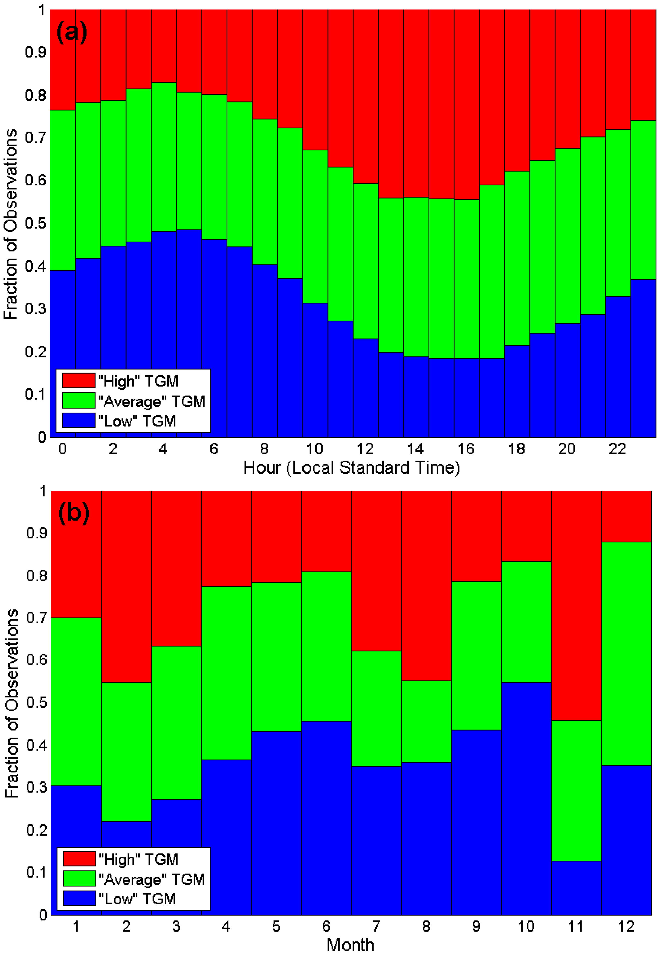
To further support this argument, Figure 6 shows the diel and monthly fractional distributions of observations of “high”, “average”, and “low” TGM concentrations, with divisions at the 67th- and 33rd-percentiles of de-trended/seasonally adjusted TGM concentrations (described above in Section 2.2 and illustrated in Figure 1) excluding data affected by forest fire smoke. Figure 6a shows the “low” TGM concentration observations typically occurred in the early morning or overnight while “high” TGM concentration observations typically occurred in the mid-day. The frequency of “average” TGM concentration observations is consistent throughout the day as indicated in Figure 6a. This is not to say that “average” TGM concentration observations do not exhibit a diel trend, but rather that “average” TGM concentrations can be observed with the same frequency at any time of day. In contrast, Figure 6b shows that the “high”, “average”, and “low” TGM concentration subsets do not have any clear seasonal trend. Figure 6b emphasizes that “low” TGM concentration observations are distributed more or less equally over the course of the year, suggesting “low” TGM concentrations originating from arctic regions are more likely due to generally cleaner air than to AMDEs. Had the “low” TGM concentration observations been a result of local/regional AMDEs, one would expect to see the highest frequency of “low” TGM concentration observations during daylight hours. Likewise, had the “low” TGM concentrations been a result of arctic air transported into the region after arctic AMDEs, one would expect to see the highest frequency of “low” TGM concentration observations during the spring. Note that Figure 3 also indicates that lower TGM concentration observations are not particularly common in the spring.

Figure 6. (a) Diel and (b) monthly fractional distribution of “high”, “average”, and “low” de-trended/seasonally adjusted TGM concentrations as defined in the text. These plots exclude data affected by forest fire smoke.

Figure 6. (a) Diel and (b) monthly fractional distribution of “high”, “average”, and “low” de-trended/seasonally adjusted TGM concentrations as defined in the text. These plots exclude data affected by forest fire smoke.

Figure 6a indicates again that, in general, local daytime oxidation by ozone is an unviable reaction mechanism for TGM depletion observed at Patricia McInnes. The diel trend in Figure 6a also supports conclusions that TGM is driven by diel trends affecting underlying surface-air flux and long-range transport of global atmospheric mercury. In other words, a diel trend is superimposed on the TGM concentration time series that undergoes lower frequency oscillations as air with higher or lower TGM concentrations move over the monitoring station. The back trajectory analysis above also supports this conclusion, in that the lowest TGM values came with air that has passed through arctic regions of northern Canada, and are thus presumably cleaner than air originating from more populated regions. GEM oxidation chemistry may still be occurring locally, but it is difficult to speculate to what extent it occurs, if at all, without speciated mercury measurements providing GOM concentration data. Also, this dataset cannot provide any insight to the role of particulate bound mercury in the area. Mercury speciation measurements will form a future component of the Joint Canada-Alberta Implementation Plan for Oil Sands Monitoring, and that future work may provide further information to more definitively understand any local mercury chemistry taking place in the region with associated effects on local mercury deposition.

3. Experimental Section

3.1. Site Description

Fort McMurray—Patricia McInnes station (56°45′7′′N, 111°28′34′′W; elevation 362 m; see Figure 7) is an ambient air quality monitoring station operated by WBEA and located in a neighbourhood in the northwest quadrant of Fort McMurray, Alberta (2011 population: 61,374). As a community-based station, as opposed to an air permitting approval-based station, Patricia McInnes station is surrounded by housing to the immediate north, south, and east (325°–0°–245°), and a recreational park and woodland to the immediate west (245°–325°). Fort McMurray is located in the Regional Municipality of Wood Buffalo on the Athabasca River approximately 30 km south of the oil sands developments and approximately 380 km north-northeast of Edmonton, Alberta. The area is within the Boreal Plains Ecozone of Canada in which balsam fir/poplar, white/black spruce, white birch, and trembling aspen are common [33]. Under the Köppen climate classification system, Fort McMurray is categorized as humid continental climate bordering on subarctic with large seasonal temperature differences ranging from the mean winter minimum of −20.7 °C to the mean summer maximum of 22.5 °C [34].

3.2. Methods

Ambient total gaseous mercury (TGM) concentrations are measured as part of Environment Canada’s contribution to the Canada-Alberta Joint Oil Sands Monitoring Plan with the assistance of WBEA. Environment Canada operates Tekran Model 2537 Mercury Vapor Analyzers in continuous 5-minute intervals following the Canadian Atmospheric Mercury Measurement Network (CAMNet) TGM guidelines for instrument configuration and maintenance [7,35]. Measurements have been ongoing at WBEA’s Patricia McInnes station since October 2010 and continue today with technical support from the WBEA staff. This study considers data from 21 October 2010 through 31 May 2013, inclusively. The quality controlled TGM data is publicly available on the Canada-Alberta Joint Oil Sands Environmental Monitoring Information Portal [36].

Figure 7. Map of the area showing Patricia McInnes Station (A), Athabasca Valley Station (B), Fort McMurray Airport (C), and Fort McKay (D). Inset map of Alberta shows study area in relationship to Edmonton (E). Fort McMurray and oil sands deposits and production areas are shaded according to the legend [37].

Figure 7. Map of the area showing Patricia McInnes Station (A), Athabasca Valley Station (B), Fort McMurray Airport (C), and Fort McKay (D). Inset map of Alberta shows study area in relationship to Edmonton (E). Fort McMurray and oil sands deposits and production areas are shaded according to the legend [37].

Table 6 lists TGM and other measured parameters used in this study, with station, operator, and source details. Air quality parameters include nitrous oxide (NO), nitrogen dioxide (NO₂), oxides of nitrogen (NO_X), ozone (O₃), fine particulate matter (PM_2.5), sulphur dioxide (SO₂), total hydrocarbon (THC), total reduced sulphur (TRS), ammonia (NH₃), and carbon monoxide (CO). Meteorological parameters include temperature (T), relative humidity (RH), wind speed and direction, solar radiation, and snow depth. Most of these variables were chosen due to the fact they were measured at Patricia McInnes station. Solar radiation, snow depth, and RH measured at nearby stations were included due to associations with TGM concentration noted in previous work [19]; CO was included as a forest fire tracer as noted below. The data source of each parameter, as listed in Table 6, provides corresponding details on instrumentation; all public data has been quality controlled by the respective operator and provided as hourly averages from continuous instrumentation. Wind speed and direction are hourly vector averages. Measurement probes and sampling inlets are approximately 2–3 m above ground at each station.

Elevated concentrations of PM_2.5 and CO were used as tracers to determine the presence of forest fire smoke in the vicinity of the monitoring station, corroborated with archived forecasts of ground-level PM_2.5 concentrations due to forest fire smoke [38].

Table 6. Summary of data sources.

Parameter	Station	Latitude	Longitude	Elevation	Operator	Source
TGM	Fort McMurray—Patricia McInnes	56.75°N	111.48°W	362 m	Environment Canada	JOSMa
NO					Wood Buffalo Environmental Association	CASAb
NO2
NOX
O3
PM2.5
SO2
THC
TRS
Temperature
Wind Speed
Wind Direction
NH3						WBEAc
CO	Fort McMurray—Athabasca Valley	56.73°N	111.39°W	260m	Wood Buffalo Environmental Association	CASAb
Solar Radiation	Fort McKay	57.19°N	111.64°W	269	Wood Buffalo Environmental Association	CASAb
RH	Fort McMurray Airport	56.65°N	111.22°W	369m	Environment Canada	ECd
Snow Depth

Notes: ^a Joint Oil Sands Monitoring Data Portal website [36]. ^b Clean Air Strategic Alliance website [39]. ^c Wood Buffalo Environmental Associations website [40].^d Environment Canada National Climate Data and Information Archive [41].

Table 6. Summary of data sources.

Parameter	Station	Latitude	Longitude	Elevation	Operator	Source
TGM	Fort McMurray—Patricia McInnes	56.75°N	111.48°W	362 m	Environment Canada	JOSMa
NO					Wood Buffalo Environmental Association	CASAb
NO2
NOX
O3
PM2.5
SO2
THC
TRS
Temperature
Wind Speed
Wind Direction
NH3						WBEAc
CO	Fort McMurray—Athabasca Valley	56.73°N	111.39°W	260m	Wood Buffalo Environmental Association	CASAb
Solar Radiation	Fort McKay	57.19°N	111.64°W	269	Wood Buffalo Environmental Association	CASAb
RH	Fort McMurray Airport	56.65°N	111.22°W	369m	Environment Canada	ECd
Snow Depth

Notes: ^a Joint Oil Sands Monitoring Data Portal website [36]. ^b Clean Air Strategic Alliance website [39]. ^c Wood Buffalo Environmental Associations website [40].^d Environment Canada National Climate Data and Information Archive [41].

3.3. Data Quality Assurance/Quality Control

Raw TGM data is ingested into the Research Data Management and Quality Control System (RDMQ) developed by Environment Canada [8,42] where every 5-minute measurement is manually scrutinized and flagged. As supplementation to RDMQ, raw and quality controlled air quality and meteorological data from WBEA’s Patricia McInnes air monitoring station provided various parameters with which to compare. These parameters, alongside instrument diagnostics, are compared to the flagged values in RDMQ to determine if the measurement is valid. After acceptance of a valid data point (measured over 5 min), averages are calculated for hours where three or more data points exist. If less than three data points exist in a given hour, the hour is marked as missing. A large gap in the dataset exists from 21 May 2011 to 20 October 2011. Measurements were made during this period; however, significant forest fires north of Fort McMurray and associated heavy smoke caused particles to bypass plugged particulate filters and contaminate the instrument’s gold traps. This caused lower measurements to be recorded during the 5-minute collection phase in that not all of the mercury in the ambient air was able to be pre-concentrated on the contaminated gold traps. The issue was discovered during the QC process after an increase in TGM concentrations was observed upon replacement of the gold traps in October 2011. As a result, data was invalidated back to the date in May where flow issues were first observed, and it is believed smoke first affected the gold traps. Invalidated data were not included in the analysis, statistical tests, or interpretation of results in this study.

3.4. Statistical Analyses

Principal component analyses, descriptive statistics, trend analysis, t-tests, and de-trending/seasonal adjustments were carried out with Matlab software. Several other parameters measured at Patricia McInnes and neighbouring monitoring stations (as summarized in Table 6) were used for PCA. Components identified with PCA were varimax rotated to identify a handful of the most important factors that explain the most variability in the dataset. For a detailed description of PCA, see Hair et al. [22]. By comparing how TGM concentrations load on each factor for various data subsets, one can gain an insight into which factors have the most influence over TGM concentration.

3.5. HYSPLIT Back Trajectory Analysis

The online version of the Hybrid Single Particle Lagrangian Integrated Trajectory (HYSPLIT) model [24,25] was applied using default meteorological settings, including archived meteorological data from the National Centers for Environmental Prediction’s Global Data Assimilation System using model vertical velocity for vertical motion. Archived meteorological data was provided on a 1° grid with 23 vertical levels along the pressure gradient. A separate 72-hour back trajectory was obtained for each hourly observation of de-trended/seasonally adjusted TGM concentration measured at Patricia McInnes station, excluding data associated with forest fire smoke for a total of 17,020 unique trajectories. The objective behind running back trajectories in this study was to better understand the source region(s) of air parcels impinging upon the monitor, not specifically to track regional air flows. Since the TGM monitor samples below the mixing height nearly all the time, it is important that the end point of the back trajectories also be below the mixing height. For this reason, back trajectories arrived at the monitoring station 50 m above ground level, to be generally less than the minimum mixing height at any given time of day or year [43], but also high enough to avoid model surface artifacts. The 72-hour back trajectories were chosen to provide a balance between sufficient spatial distribution of back trajectory starting points while minimizing errors associated with longer back trajectories.

Three figures are presented to show the results of the HYSPLIT back trajectory analysis. Figure 5a presents each individual back trajectory’s starting point and is colour coded based on the associated de-trended/seasonally adjusted TGM concentrations. Note that the points in Figure 5a were layered by observation—as opposed to layered by de-trended/seasonally adjusted TGM concentrations—to provide a sense of randomization to prevent visually biasing either high or low de-trended/seasonally adjusted TGM concentrations in this panel. Figure 5b uses the point density tool in ArcMap 10 and is defined by a 10 km × 10 km grid focused over western Canada. The point density tool determines the density of data points within a user defined distance from the center of a given grid cell—a neighbourhood. For Figure 5b, the point density tool is applied to the number of back trajectories within a 700 km radius neighbourhood from the center of each grid cell. The trajectory point density map may be conceptualized as a population density map where the number of back trajectory starting points is substituted for population. Figure 5b does not take into account the TGM concentrations associated with each back trajectory. A 700 km radius neighbourhood was used to provide a balance between smoothing the map of fine details that can overemphasize individual starting points without losing larger-scale features. For further details on point density mapping, see [44,45].

Figure 5c uses the combination of Figure 5a and Figure 5b to create a de-trended/seasonally adjusted TGM concentration weighted point density map, normalized by point density. In Figure 5c, each back trajectory starting point was weighted with its corresponding de-trended/seasonally adjusted TGM concentration. The de-trended/seasonally adjusted TGM concentration weighted points were then normalized by the number of trajectories in the grid cell, as determined by Figure 5b. Normalizing by the number of trajectories in the grid cell avoids biasing the map in regions where there are fewer back trajectory starting points. For each 10 km × 10 km grid cell, this process is mathematically defined as the weighted point density (in units of ng∙m⁻³∙km⁻²) divided by the point density (in units of km⁻²), to result in the normalized TGM concentrations (in units of ng∙m⁻³) as presented in Figure 5c.

4. Conclusions

Ambient concentrations of total gaseous mercury were measured at WBEA’s Fort McMurray—Patricia McInnes air quality monitoring station from 20 October 2010 through 31 May 2013. The results show that TGM concentrations are comparable to that measured at other stations in the province of Alberta. TGM concentration undergoes seasonal and diel trends, with high values in the spring and midday, and low values in the fall and early morning. Higher TGM concentrations were generally a result of forest fire smoke transported to the sampling area and other long-range transport via the southeast and west, whereas lower TGM concentrations were generally a result of cleaner air transported into the region via the arctic. There was no correlation between concentrations of TGM and other anthropogenic pollutants (i.e., NO_X and SO₂), despite the fact that the station is within an urban area and near the industrialized center of the Canadian oil sands region. Although reduced TGM concentrations were associated with reduced ozone concentrations, the data do not suggest that mercury oxidation chemistry via ozone plays a major role in the area. This work provides a critical component for future work to better understand mercury deposition and cycling within the Canadian oil sands region.