Article

Assessment of the Weather Research and Forecasting/Chemistry Model to Simulate Ozone Concentrations in March 2008 over Coastal Areas of the Sea of Japan

by
Khandakar Md. Habib Al Razi
* and
Moritomi Hiroshi
Environmental and Renewable Energy System, Graduate School of Engineering, Gifu University, 1-1 Yanagido, Gifu 501-1193, Japan
*
Author to whom correspondence should be addressed.
Atmosphere 2012, 3(3), 288-319; https://doi.org/10.3390/atmos3030288
Submission received: 9 February 2012 / Revised: 10 April 2012 / Accepted: 18 June 2012 / Published: 10 July 2012

Abstract

:
The fully coupled WRF/Chem (Weather Research and Forecasting/Chemistry) model is used to simulate air quality over coastal areas of the Sea of Japan. The anthropogenic surface emissions database used as input for this model was based primarily on global hourly emissions data (dust, sea salt, and biomass burning), RETRO (REanalysis of the TROpospheric chemical composition), GEIA (Global Emissions Inventory Activity), and POET (Precursors of Ozone and their Effects in the Troposphere). Climatologic concentrations of particulate matter derived from the Regional Acid Deposition Model (RADM2), chemical mechanism, and the Secondary Organic Aerosol Model (MADE/SORGAM) with aqueous reactions were used to deduce the corresponding aerosol fluxes for input to the WRF/Chem model. The model was first integrated continuously over 48 hours, starting from 00:00 UTC on 14 March 2008, to evaluate ozone concentrations and other precursor pollutants. WPS meteorological data were used for the WRF/Chem model simulation in this study. Despite the low resolution of global emissions and the weak density of the local point emissions, it was found that the WRF/Chem model simulates the diurnal variation of the chemical species concentrations over the coastal areas of the Sea of Japan quite well. The Air Quality Management Division of the Ministry of the Environment in Japan selected the maximum level of the air quality standard for ozone, which is 60 ppb. In this study, the atmospheric concentrations of ozone over the coastal area of the Sea of Japan were calculated to be 30–55 ppb during the simulation period, which was lower than the Japanese air quality standard for ozone.

1. Introduction

At present, more than 60 million people are added to cities each year worldwide, and approximately 325 cities have a population of more than one million, compared to 270 such cities in 1990 [1]. In recent decades, air quality has deteriorated remarkably in the large cities of developing countries. The export of air pollutants from urban to regional and global environments is of major concern because of wide-ranging potential consequences for human health and for cultivated and natural ecosystems, visibility degradation, weather modification, radiative forcing, and changes in tropospheric oxidation (self-cleaning) capacity. Rapidly increasing urbanization will be a major environmental driving force in the 21st century, affecting air quality on all scales (e.g., local, regional, and global) [1]. Large numbers of people are likely to be exposed to unhealthy ozone (O3) concentrations when ground-level ozone accumulates in urban metropolitan areas under certain weather conditions [2], and quantitative atmospheric dispersion models will be of great help to provide effective decision support systems for planners and administrators.
The main pollutants emitted into the atmosphere in urban areas are sulfur oxides (SOx), nitrogen oxides (NOx), carbon monoxide (CO), volatile organic compounds (VOCs), metal oxides, and particulate matter (PM/aerosols), mostly consisting of black carbon, sulfates, nitrates, and organic matter. The oxidization of CO, VOCs, and NOx produces ozone in the planetary boundary layer (PBL), which has an important impact on human health in urban areas. The recent economic developments of China, Korea, and Japan are very rapid due to the rapid growth of heavy industrial operations. The rapidly growing urbanization in these countries will cause wide-ranging potential consequences in terms of environmental problems. These areas have been suffering from severe air pollution problems for the past decade, such as high particulate matter (PM) concentrations and poor visibility [3,4,5,6]. As industrial activity and the number of automobiles increases, the emission of volatile organic carbons (VOCs) and NOx (NO + NO2) will also significantly increase. Both VOCs and NOx play critical roles in ozone formation in the troposphere [7,8], and the variations in their concentrations and the ensuing effects on the ozone production rate can be characterized as either NOx-sensitive or VOC-sensitive [7,9,10,11,12]. Thus, obtaining a better understanding of the relationship between ozone precursors (VOCs, NOx) and ozone formation in east Asia is one of the critical pre-required pieces of information necessary to develop effective ozone control strategies [13,14,15].
In Japan, VOC, NOx, and SOx were categorized as hazardous air pollutants (HAPs) in 1996 and are on the list of Substances Requiring Priority Action published by the Central Environmental Council of Japan [16]. The Central Environmental Council published the second report on the “Future direction of measures against hazardous air pollutants” in October 1996. The second report also proposed that voluntary actions to reduce emissions, as well as investigations of hazards, atmospheric concentrations and pollution sources of those substances, should be promoted. Although industrial emissions of VOCs, NOx, and SOX in Japan have been decreasing in recent years, primarily due to voluntary reductions from industrial sources, the risks of exposure to these pollutants have remained largely unknown. In this study, a rapid change of ozone and its precursors were simulated during the spring of 2008. The simulation results contribute to a better understanding of ozone variability in coastal areas of the Sea of Japan [17]. A three-dimensional chemical/dynamical regional model (WRF/Chem V-3.3) was applied to analyze the causes of the rapid changes in ozone during this period.
Ozone is not emitted directly into the air; instead, it forms in the atmosphere as a result of a series of complex chemical reactions between oxides of nitrogen (NOx) and hydrocarbons, which together are precursors of ozone. Ozone precursors have both anthropogenic (man-made) and biogenic (natural) origins. Motor vehicle exhaust, industrial emissions, gasoline vapors, and chemical solvents are some of the major sources of NOx and hydrocarbons. Many species of trees and other plants emit hydrocarbons, and fertilized soils release NOx [18,19].
In the presence of ultraviolet sunlight (), oxygen (O2) and nitrogen dioxide (NO2) react in the atmosphere to form ozone and nitric oxide (NO) [18,19]. The resultant ozone reacts with NO to form nitrogen dioxide. A steady state is attained through these reactions:
NO2 + → NO + O
NO + NO2 + H2O → 2HONO
HONO + → NO + OH
O + O2 → O3
CO + 2O2 → CO2 + O3
O3 + NO → NO2 + O2
Even in the absence of anthropogenic emissions, these reactions normally result in a natural background ozone concentration of 25 to 45 ppb [20,21]. Ozone cannot accumulate further unless volatile organic compounds (VOCs), which include hydrocarbons, are present to consume or convert NO back to NO2 [19,22,23], as in the following:
VOC + NO → NO2 + other products
This equation is a simplified version of many complex chemical reactions. Because NO is consumed by this process, it is then no longer available to react with ozone. When additional VOCs are added to the atmosphere, a greater proportion of the NO is oxidized to NO2, resulting in a greater amount of ozone formation. Anthropogenic sources of NO lead to higher levels of NO2 in the atmosphere, and this NO2 is then available for photolysis. The formation and increase in ozone concentrations occur over a period of a few hours. Shortly after sunrise, NO and VOCs react in the presence of sunlight to form ozone. Throughout the morning, ozone concentrations increase while NO and VOCs are depleted. Eventually, either the lack of sunlight, NO, or VOCs limits the production of ozone. This diurnal cycle varies greatly depending on site location, emission sources, and weather conditions. Precursor emissions of NO and VOCs are necessary for ozone to form in the troposphere. Understanding the nature of when and where ozone precursors originate may help forecasters factor in day-to-day changes in emissions. For example, if region’s emissions are dominated by mobile sources, then emissions, and thus the ozone that forms from them, may depend on day-to-day commuting patterns. The primary sources of NOx production are combustion processes, including industrial and electric generation processes, and mobile sources such as automobiles [24]. Mobile sources also account for a large portion of VOC emissions. Industries such as the chemical industry or others that use solvents also account for a large portion of VOC emissions. Biogenic VOC emissions from forested and vegetation areas may impact urban ozone formation in some parts of the country. Biogenic NOx emission levels are typically much lower than anthropogenic NOx emission levels [24].
In this study, a preliminary evaluation of the model performance was performed by comparing results to the online observations obtained from different monitoring stations over the past few years (2000–2008) in Japan. The spatial and temporal dynamics were studied using simulations performed with the Weather Research and Forecast (WRF) model [25] coupled with the Chemistry model (WRF/Chem) [26]. Due to the geographical complexity of the study area, an important part of the study was also to evaluate the model’s ability to represent the measured meteorological conditions and surface ozone levels.
The development and occurrence of photochemical pollution episodes have been studied using air quality models (AQM) as they incorporate the contributing atmospheric physical and chemical processes [27,28,29,30,31,32]. The fully coupled weather chemistry model, WRF/Chem, is the next generation model currently used by many researchers for air quality studies [33,34,35,36,37] over different regions. Misenis [35] used WRF/Chem to study the air quality of the Houston–Galveston area and reported that the model planetary boundary layer (PBL) and land surface model (LSM) schemes affected the simulation of chemical species. Their study indicated that the Yonsei University non-local diffusion PBL scheme has given better results for meteorological variables than the Mellor-Yamada-Janjic PBL scheme for the ozone predictions. Jiang [36] studied a continuous photochemical pollution episode in Hong Kong using WRF/Chem to examine the meteorological processes contributing to the formation of high ozone and reported that the northerly air stream associated with high temperatures, stable boundary layer and clear sky conditions favored the high ozone formation in Hong Kong city. De Foy [37] evaluated the WRF model for the complex wind flows in the Mexico City basin area with data from field campaigns using statistical techniques, cluster analysis of flow trajectories and concentration measurements. Their study of ozone showed the influence of the local and regional scale circulations and their modulation by the synoptic–scale flow patterns to govern the short-range transport in the Mexico City region. Tie [38] studied the performance of the WRF/Chem for the simulation of ozone and its precursors in the Mexico City region using in situ aircraft measurements of chemical species. They reported that the model was able to capture the timing and location of the ozone concentrations, their association with city plumes and that the model underestimated the ozone mixing ratios by about 0–25%. Zhang [39] studied the air quality over Mexico City using WRF/Chem and reported that the model performs much better during daytime than nighttime for both chemical species and meteorological variables and different combinations of the available PBL and land surface schemes did not reduce the errors.
Chatani and Sudo [40] observed and analyzed the seasonal variation of ozone concentration in the Japan domain by using the WRF/Chem, CHASER model with monitoring station data during 1996–2005. They tried to evaluate the performance of the WRF/Chem, CHASER model with monitoring data during this period. Masanori [41] evaluated vertical ozone profiles simulated by WRF/Chem using Lidar observation over the Kanto region of Japan on 27–29 July and 16–21 August 2005. Kurokawa [42] showed the influence of meteorological variability on interannual variations of the springtime boundary layer ozone over Japan between 1981–2005. Kurokawa [43] depicted an analysis of episodic pollution of photochemical ozone during 8–9 May 2007 over Japan using the nesting RAMS/CMAQ modeling system. Hayasaki [44] described Episodic pollution of photochemical ozone during 8–9 May 2007 over Japan. Saikawa [45] analyzed the impact of China’s vehicle emissions on regional air quality in 2000 and 2020. It is evident that the early research work on ozone simulation by WRF/Chem in the Japan domain did not show any time series ozone concentration with observation data to find out an ozone episode. However, the use of WRF/Chem to predict the ozone concentration in Japan domain is very rare.
In this study an attempt has been made to examine the evolution of surface ozone and other precursor emissions like NOx over the Coastal Areas of the Sea of Japan using WRF/Chem, an online chemistry model. The performance of WRF/Chem in the simulation of ozone concentration distribution in the region that have occurred during the spring (middle of March) condition and the results from this study could provide useful information about ozone formative meteorological processes to air quality regulatory agencies and health administrators. The spring climate in the study region is characterized with strong land–ocean thermal gradients and the resulting mesoscale sea breeze circulation. The concentration distribution of ozone in 14–16 March 2008 during spring with sufficient observations was selected to assess the model performance.

2. Model Description

The Weather Research and Forecasting (WRF) model is a mesoscale numerical weather prediction system designed to serve both operational forecasting and atmospheric research needs. The development of the WRF model has been a collaborative partnership, principally among the National Center for Atmospheric Research (NCAR), the National Oceanic and Atmospheric Administration (NOAA), the National Center for Environmental Prediction (NCEP), the Forecast Systems Laboratory (FSL), the Air Force Weather Agency (AFWA), the Naval Research Laboratory, Oklahoma University, and the Federal Aviation Administration (FAA). The WRF model is a fully compressible and Euler nonhydrostatic model. It calculates winds (u, v, and w), the perturbation potential temperature, the perturbation geopotential, and the perturbation surface pressure of dry air. It can also optionally output other variables, including turbulent kinetic energy, the water vapor mixing ratio, the rain/snow mixing ratio, and the cloud water/ice mixing ratio. The model physics include bulk schemes, mixed-phase physics of cloud-resolving modeling, and multi-layer land surface models ranging from a simple thermal model to full vegetation and soil moisture models. The full vegetation and soil moisture land surface models can include snow cover and sea ice, turbulent kinetic energy predictions or non-local K schemes for planetary boundary layer calculations, long wave and shortwave schemes with multiple spectral bands, and a simple shortwave model. On the other hand, the WRF Preprocessing System (WPS) is used to prepare a domain (region of the earth) for WRF. The WPS consists of three independent programs: geogrid, ungrib, and metgrid. The purpose of geogrid is to define the simulation domains and interpolate various terrestrial data sets to the model grids. The ungrib program reads GRIB files, degribs the data, and writes the data in a simple format, called the intermediate format. The metgrid program horizontally interpolates the intermediate-format meteorological data that are extracted by the ungrib program into the simulation domains defined by the geogrid program. A detailed description of the WRF and WPS model can be found on the WRF website [26].
In addition to a dynamical calculation, a chemical model (WRF/Chem) is fully (on-line) coupled with the WRF model. A detailed description of WRF/Chem is given by Grell et al. [26]. The version of the model (version 3.3) used in the present study includes simultaneous calculations of dynamical parameters (e.g., wind, temperature, boundary layer, and clouds), transport (advective, convective, and diffusive), dry deposition [46], gas phase chemistry, radiation and photolysis rates [47,48], and surface emissions, including online calculations of biogenic emissions. Ozone chemistry is represented in the model by a modified Regional Acid Deposition Model version 2 (RADM2) gas-phase chemical mechanism [49], which includes 158 reactions among 36 species, in conjunction with the Secondary Organic Aerosol Model (MADE/SORGAM) of aqueous reactions [50].

3. Simulation Method

3.1. Model Settings and Initialization

The WRF/Chem simulation in this study simulated the coastal areas of the Sea of Japan (latitude 31.4°N–45.0°N and longitude 129.3°E–146.2°E), which is a marginal sea of the western Pacific Ocean, bordered by Japan, the Korean Peninsula and Russia, and is referred to in South Korea as the East Sea [51,52].
Figure 1. The nesting domain setting of the model.
Atmosphere 03 00288 g001
In this study, the model was used to simulate medium-scale and regional circulation influenced by the complex terrain within and around the coastal areas of the Sea of Japan during the period from 00:00 UTC (Coordinated Universal Time) [53] on 14 March 2008 to 00:00 on 16 March 2008; Japan Standard Time (JST) [54] is the standard time zone of Japan and is 9 hours ahead of UTC. One nesting domain was defined using the Lambert projection, which can be observed in Figure 1. The domain covers the coastal area of the entire Japanese side and a part of the Korean side of the Sea of Japan, with the center point at latitude 38.5°N, longitude 137.60°E. The domain settings and configuration options are shown in Table 1. The initial and lateral boundary conditions for the meteorology component are taken from the National Centers for Environmental Prediction (NCEP) Final (FNL) Global Analysis data available at 1° resolution and at six hour intervals. The ideal concentration profiles [55] were used as initial and boundary conditions of the chemical species. A total of 35 vertical levels with 10 levels in the lower atmospheric region (below 800 mbar) were considered in the model.
Table 1. WRF/Chem model domain settings and configuration options.
Horizontal grid (x, y)75, 70
Grid spacing22 km
Meteorological time step180 s
Chemical time step180 s
MicrophysicsWSM3-class simple ice scheme [56]
Advection scheme5th horizontal/3rd vertical [57,58]
Long wave radiationRRTM [59]
Shortwave radiationGODDARD [60,61]
Surface layerMoni-Obukhov (Janjic Eta) [62]
Land surface modelNOAH [63]
Boundary layerMellor-Yamada-Janjic TKE [64,65]
Cumulus parameterizationGrell-Devenyi ensemble scheme [66]
Chemistry optionRADM2 [67]
Dry depositionWesley, 1989 [68]
Biogenic emissionsGuenther scheme [69,70]
Photolysis optionMadronich, 1987 [71]
Aerosol optionMADE/SORGAM [72]
Models will have spin-up time; that is the time needed to adjust to forcing. In weather prediction, the model physics will spin up a velocity field in balance with the density field, even in the absence of forcing. As forcing is applied, the velocity field will respond to it initially with transient flows that may not be realistic although continuously changing. For this reason, the model simulation was started from 00:00 UTC on 6 March to 00:00 UTC on 16 March, where the first 8 days simulation results were not used in this study. The model is executed with 8 days spin-up to achieve stabilized results of this study.
The chemistry is initialized with idealized profiles, with the anthropogenic emissions data taken from the global emission data “prep_chem_sources” described in Section 3.2. The data are interpolated to model grids using the emissions processing program available with WRF/Chem. The biogenic emissions are calculated using the scheme of Guenther et al. [69,70]. WRF/Chem simulates concurrently the meteorological conditions and chemistry of atmospheric species from emission, through transport and a variety of chemical reactions, to the removal by wet or dry deposition. The Weather Research and Forecasting model [25] serves as a meteorological module for WRF/Chem. In this study, cloud and the precipitation formation process were simulated by the WSM3-class simple ice scheme [56] that allows for mixed phase processes and the coexistence of supercooled water and ice. To consider the impact of cumulus convection, despite convection only occurring on a few days during 14–16 March, the cumulus ensemble approach had been used [62]. Shortwave radiation was determined by the Goddard two stream multi-band scheme [60,61] and RRTM scheme [59], respectively, that considers, among other things, cloud effects and ice-fog. Long wave radiation was treated with the Rapid Radiative Transfer Model [59], that considers multiple spectral bands, trace gases, and microphysical species. Turbulent processes in the atmospheric boundary layer were determined using the Mellor-Yamada-Janjic TKE scheme [64,65]. However, the Monin-Obukhov similarity hypothesis was used to describe the turbulent processes in the atmospheric surface layer, where Zilitinkevich’s thermal roughness length concept was considered for the underlying viscous sublayer [65]. The exchange of heat and moisture in the land atmosphere interface was described by the Noah land surface model (NOAH) [63] which calculates soil temperature and moisture states, including frozen soil physics. Its multi-layer snow model and one-layer vegetation model considers snow and vegetation processes, respectively. The chemistry options used in the model are the Regional Acid Deposition Model version 2 (RADM2) gas-phase chemical mechanism [67] and Madronich photolysis scheme [71]. For the present study, the MADE/SORGAM [72] aerosol module is included. The chemistry was initialized with idealized profiles. The various options used in the model are given in Table 1.

3.2. Data Acquisition and Pre-Processing of Emissions

The linkages in the formation and transport of pollution between the local, regional and global scales are receiving increasing recognition and a variety of atmospheric chemistry models address these aspects. This modeling effort puts new demands on the emission inventories that are used as input to these models. The inventories need to be accurate at the local scale yet also cover the entire globe with a consistent approach.
The GEIA (Global Emissions Inventory Activity)/ACCENT (European Network of Excellence on Atmospheric Composition Change) data portal is a cooperative project that provides surface emission data (total and gridded data) for the main emission categories (total anthropogenic, total biomass burning, biogenic, and oceans) at global or regional scales from several inventories (e.g., RETRO, POET, EDGARFT2000, GFEDv2, and GEIA v1) (Table 2).
The use of a global emissions data set has recently been added to the WRF/Chem model options. The global emissions data are from the REanalysis of the TROpospheric (RETRO) chemical composition data collected over the past 40 years and the Emission Database for Global Atmospheric Research (EDGAR). Both RETRO and EDGAR provide global annual emission data of several greenhouse gases (e.g., CO2, CH4 and N2O) as well as some precursor gases on a 0.5° × 0.5° (RETRO) or a 1° × 1° (EDGAR) grid. In the present study, a simple grid-mapping program was used in the WRF/Chem model. This program, called “prep-chem-sources” for global emission data (dust, sea salt, biomass burning), was developed at CPTEC, Brazil and is available to WRF/Chem model users. The “prep-chem-sources” is an emission data generator package to provide gridded emission fluxes (kg/m2) which assimilates the inventory works (Table 2) of biomass burning and wildfire emission data from anthropogenic and biogenic sources [73,74].
Table 2. Global inventories offered by the GEIA/ACCENT data portal.
InventoryCategories Spatial resolution Temporal resolution
POET [75,76]Anthropogenic biomass burning (natural) 1 × 1Annual (anthro.), monthly (biom. burn.), monthly (natural)
RETRO [77]Anthropogenic biomass burning 0.5 × 0.5Monthly
EDGAR [78 ,79,80]Anthropogenic biomass burning 1 × 1Annual
GFED v2 [81,82]Biomass burning/wildfire emission 1 × 1Monthly
CO2 [83] Anthropogenic 1 × 1Annual
GEIA v.1 [79]Anthropogenic biomass burning naturally 1 × 1Annual + monthly for NOx, SO2, and nat. VOC

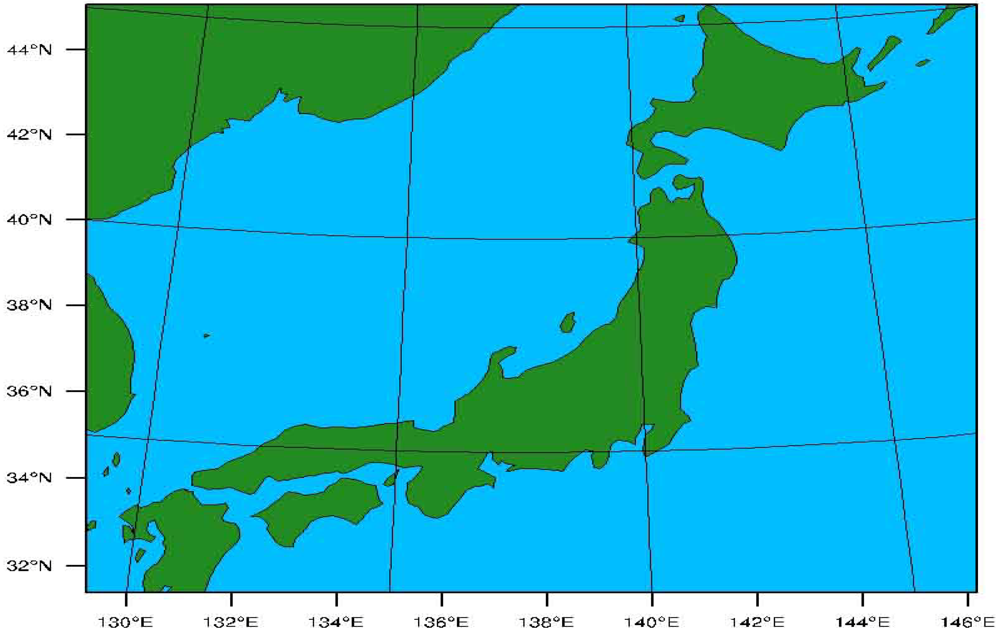
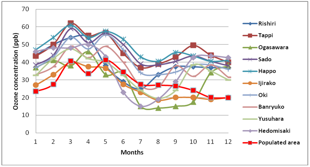
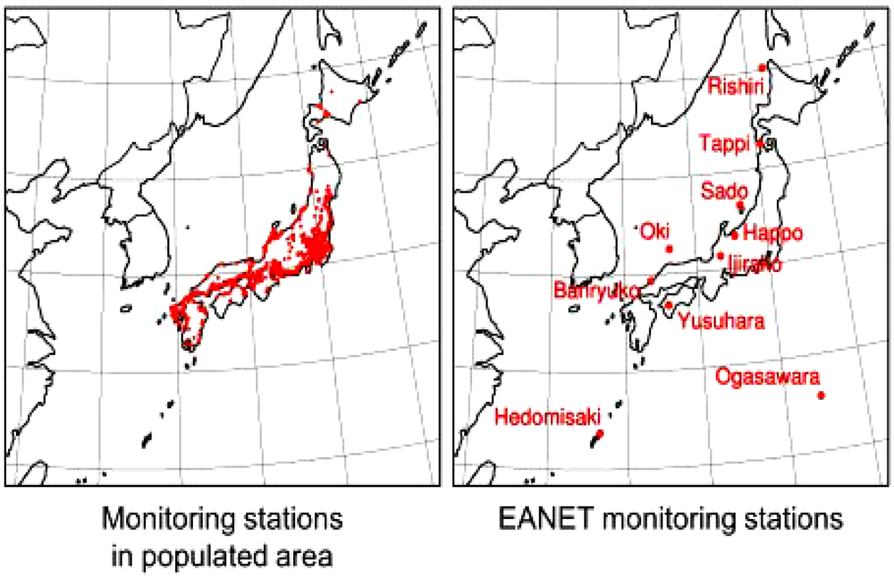
4. Observation of Ozone Concentrations over Japan

Annual and monthly pollutant concentrations observed at monitoring stations operated by Japanese local governments and the Japanese Meteorological Agency [84,85] (JMA) are available on the website [86]. This site contains data that has been collected since 1970, which are valuable for evaluating the long-term or short-term trends of pollutant concentrations in Japan. Based on this database, the Japanese government has annually reported surface ozone levels in Japan, with the long-term trend showing that these ozone levels have increased over time [87]. The first observation data set of 1,045 monitoring stations that continued to monitor photochemical oxidants between 1996 and 2008 were used in this study to investigate the pattern of ozone concentrations in March and to compare it with the simulation results. Most of the monitoring stations are located in populated coastal areas in Japan, as shown in the left map of Figure 2, because these stations are operated primarily to ensure adherence to environmental quality standards (EQSs). This database has been compiled from surface ozone concentrations recorded as daytime and nighttime averages and from the maximum concentrations of photochemical oxidants. Daytime corresponds to a twelve-hour period from 06:00 a.m. to 06:00 p.m. and time corresponds to a twelve-hour period from 06:00 p.m. to 06:00 a.m. of Japan Standard Time. Photochemical oxidants include other trace oxidants such as H2O2 and peroxyacyl nitrates (PANs), but instruments that detect only ozone have been officially approved by the Japanese government because differences in concentrations of photochemical oxidants and ozone are expected to be small [40]. Therefore, differences in concentrations between ozone and photochemical oxidants can be ignored for monthly variations in observed surface ozone concentrations. Additionally, the second observation data set of the Acid Deposition Monitoring Network in East Asia (EANET) was prepared to compare with the WRF/Chem simulation results, whereas the EANET operates monitoring stations located primarily in remote areas. Observed concentrations of surface ozone at 10 EANET monitoring stations in Japan were used to validate the performance of the simulation in Japanese background areas from 2000–2008. The locations of EANET monitoring stations are shown in the middle map of Figure 3. They are scattered in remote areas throughout Japan.
Figure 2. The locations of the monitoring stations in a populated area and of the EANET monitoring stations in Japan that were used in this study [40].
Atmosphere 03 00288 g002
The concentrations of surface ozone at EANET monitoring stations in Japan show seasonal variations, with low values in the summer (August) and higher values in the spring (Middle of March). The average ozone concentrations in March at different EANET monitoring stations were found to be approximately 37 to 55 ppb, compared to approximately 33.5 ppb in populated Japanese areas. Figure 3 shows monthly variations of observed surface ozone concentrations, averaged over 2000–2008 at each of 10 EANET monitoring stations. The red line in Figure 3 shows monthly variations of observed concentrations of surface ozone above populated Japanese areas averaged over 1996–2008.
Figure 3. Monthly variations of observed concentrations of ozone averaged over 2000–2008 at each of 10 EANET monitoring stations. The red line shows monthly variations of observed concentrations of ozone averaged over 1996–2008 above populated Japanese areas.
Atmosphere 03 00288 g003
The two observation data sets have shown that there have been air pollution episodes in the middle of March at most of the monitoring stations, in which the concentrations of ozone, nitrogen dioxide (NOx), volatile organic compounds (VOCs) and particulate matter (PM) are considerably high, hence causing lower visibility [86]. In this paper, a serious and continuous photochemical pollution episode in Japan during the anti-cyclone of 14–16 March 2008 was investigated using the WRF/Chem. Chatani and Sudo [40] observed and analyzed the ozone and other trace gas concentrations, as well as the corresponding weather conditions in this heavy-pollution episode. Our aim was to further understand the physical and chemical mechanisms of this episode by use of the new generation air quality model WRF/Chem. In Section 6.2, the simulation results were carefully compared with observation data and analyzed with the focus on local chemical production and regional transport.

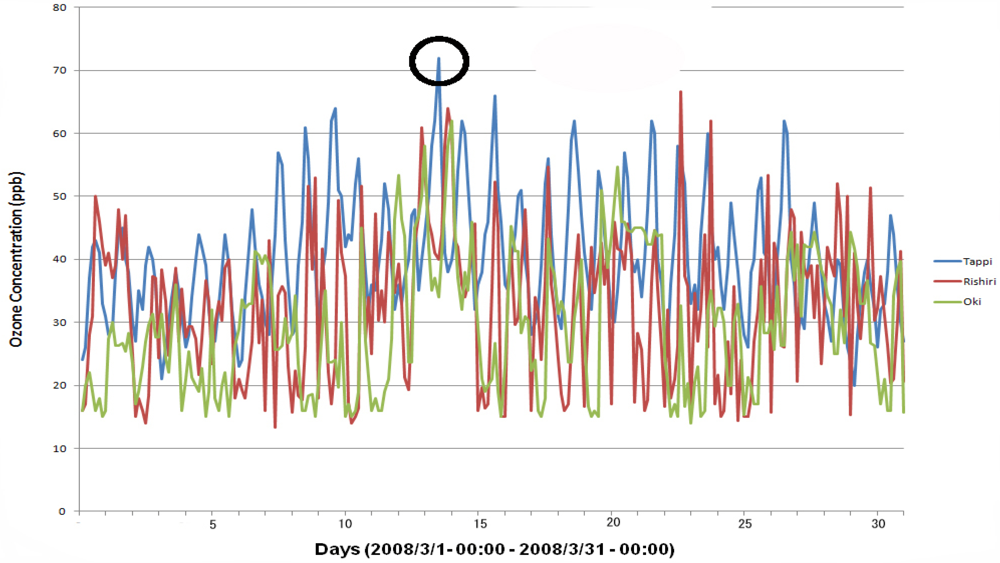
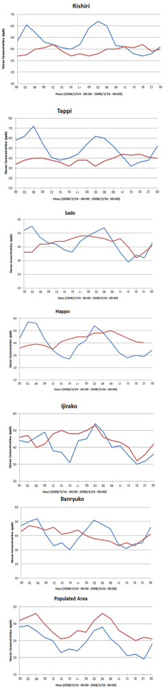
5. Characteristics of Ozone Episodes

The past several year standard ozone average of two different data sets of different monitoring stations (Figure 3) shows an average monthly variation of observed ozone concentrations. From analysis of air pollution records of the last few years, the monthly average concentration of ozone is higher in March in most of the EANET monitoring stations and the monitoring stations in the populated area. Figure 3 was prepared by the data set of monthly average ozone concentrations from 2000 to 2008 of 10 EANET monitoring stations and of the data set of monthly average concentration from 1996 to 2008 for the 1,045 monitoring stations in the populated area. Due to the trends of higher ozone concentration in March in Japan [40], an attempt has been taken to examine the evolution of surface ozone from 14 to 16 March 2008 by WRF/Chem simulation. The highest ozone concentration occurred from 14 to 16 March 2008, lasting for 2–3 days. These monitoring stations are Rishiri, Tappi, Happo, and Banryuko and are representative of the coastal region; Ijirako and Yusuhara are the representative of the inland area; Sado, Oki, Ogasawara, Hedomisaki are located in the island. Prior to the episode, the surface ozone concentrations were low on 13 March (about 50–60 ppb) and exceeded to 60 ppb at the monitoring stations Rishiri, Tappi and Oki on March 14 and 15 and reached 72 ppb on 14 March at Tappi. The peak higher value of ozone concentration was identified 72 ppb on March 14 at Tappi, which could be called an episode (Figure 4). Figure 4 shows time series (3 hours interval) zone concentrations from 00:00 UTC on 1 March to 00:00 UTC on 31 March of 2008. The black circle on Figure 4 shows the peak ozone concentration (72 ppb). Although these periods do not characterize a very severe ozone episode, they are considered important as the hourly average ozone values at 2 EANET monitoring stations exceeded 60 ppb, a threshold which can seriously affect people suffering from respiratory deficiencies [88,89] and therefore indicate moderate severe ozone pollution for human health. However, the hourly average ozone concentration at all EANET monitoring stations exceeded 50 ppb, which exceeded the air quality standard of Japan for hourly average ozone concentrations [90].
Figure 4. Time series (3 hours interval) zone concentrations from 00:00 UTC on 1 March to 00:00 UTC on 31 March of 2008 at Tappi, Rishiri, Oki. The black circle shows the peak ozone concentration (72 ppb) on 14 March at Tappi, which could be called an episode.
Atmosphere 03 00288 g004

6. Modeling Results and Discussion

6.1. Ozone Concentrations Based on WRF/Chem Simulations

Figure 5, which is the composite image from the modeling results of single nesting domains, illustrates the spatial distribution of surface ozone concentrations averaged from 00:00 UTC on 14 March (9:00 a.m. Japanese Standard Time) to 00:00 UTC on 16 March 2008. To display the time evolution of the simulated ozone concentrations, Figure 5 shows the structure of the ozone field from 03:00 UTC on 14 March to 00:00 UTC on 16 March 2008 at 1,000 mbar atmospheric pressure levels (vertical level z = 1) by using the WRF/Chem post-processing tools Grid Analysis and Display System (GrADS). This level was chosen to emphasize the transport processes across the coastal areas of the Sea of Japan relative to surface processes. However, most of the EANET monitoring stations are located in the mountainous area about 80–120 meters above ground level. In the present study, the WRF/Chem model was used to simulate the spatial and temporal variations of surface ozone and its precursor pollutants NOx over Coastal Areas of the Sea of Japan. Ozone in the high concentration zone was calculated mainly over the Sea of Japan oceanic regions on 14 March and was found to be 40 to 45 ppb, as shown in Figure 5. At 09:00 UTC on 14 March, ozone started to build up in the boundary layer with concentrations of 44 ppb near the Korean Peninsula. An anticyclone [91] induced the high-ozone region to rotate clockwise from the Korean Peninsula (09:00 UTC on 14 March) to the southwestern part of the Honshu island of Japan (15:00 UTC on 14 March) and then to the Pacific Ocean (06:00 UTC on 15 March). Due to the long lifetime of ozone (about a week) in the troposphere, the distribution of ozone concentrations was greatly influenced by the airflow of the anticyclone. According to Figure 5, cyclonic winds (anticlockwise rotation) are noted at 138.4°E, 41.6°N. After 00:00 UTC on 15 March, ozone concentrations (50 ppb) were found to be highest in the southern part of Honshu. Another small area of high ozone concentrations built up near the coastal area of the eastern part of Honshu (00:00 UTC on 14 March), which stagnated for several hours and then moved to the Pacific Ocean; the entire polluted air mass was pushed eastwards by a cold front coming from the northwest [92]. In addition, the level of primary pollutants, such as NOx, was relatively lower over the ocean, resulting in a lower consumption of ozone; thus, the highest concentrations of ozone were found over the ocean. An important fact revealed by the simulated results was that ozone levels did not reach extreme values (70–90 ppb) [93]. The Air Quality Management Division of the Ministry of the Environment in Japan selected the maximum level of the air quality standard for ozone, which is 60 ppb [90]. In this study, the range of atmospheric concentrations of ozone over the coastal areas of the Sea of Japan were calculated using the WRF/Chem model to be 30–55 ppb during the simulation period, which was lower than the Japanese air quality standard for ozone.
Figure 5. Ozone concentrations (ppb) over the coastal areas of the Sea of Japan from 03:00 UTC on 14 March to 00:00 UTC on 16 March (3 hours interval), 2008, based on the simulation results of the WRF/Chem model.
Atmosphere 03 00288 g005

6.2. Comparison of WRF/Chem Simulation Results with Monitoring Data

The time series of model-simulated ozone for the 48 hour period (3 hours interval) from 00:00 UTC on March to 00:00 UTC on 16 March of 2008 corresponding to the observation site are shown in Figure 6. In this study, ozone concentration data at the location of EANET monitoring stations calculated by the WRF/Chem were taken at 1,000 mbar atmospheric pressure levels (vertical level z = 1). On the other hand, average ozone concentration data at the location of the Japanese populated area were extracted at the ground level from the NetCDF files of WRF/Chem output, because these monitoring stations are located at the ground level of urbanized areas in Japan. This time series shows that the surface ozone gradually decreased from 18:00 UTC onwards, reaching a minimum level around midnight, and stayed nearly constant until dawn, and gradually increased from dawn to noon, reaching a maximum around 12:00 UTC. It is noted that the model simulated a maximum of 50 ppb as compared to an observational maximum of 70 ppb.
Figure 6 shows three hours average ozone concentrations at seven EANET monitoring station sites and the monitoring stations in the populated area in Japan during this period. The ozone concentrations were relatively low at night time (about 15–40 ppb), it rose during daytime and reached the highest ozone concentration (about 55–70 ppb). Figure 6 gives the hourly average concentrations of ozone observed at the seven EANET monitoring station sites as well as the monitoring stations in the populated area in Japan compared with WRF/Chem simulation. The surface ozone levels (hourly average value) exceeded 50 ppb in most of the EANET monitoring stations in Japan. The time series of ozone concentrations (3 hours average) during the above episodes at 7 EANET monitoring stations and monitoring stations in the populated area are shown in Figure 6.
Figure 6 shows the accuracy of the WRF/Chem simulation results compared with the observation data of some monitoring stations. Although the fine resolution afforded by the WRF/Chem model effectively titrates ambient ozone and moves the simulated concentrations of surface ozone closer to the observed values, the WRF/Chem model underestimated surface ozone concentrations in March over most of the EANET monitoring stations in Japan and overestimated concentrations over the populated areas of Japan. Figure 6 shows a reasonable agreement with the monitoring data with respect to predicting localized atmospheric ozone concentrations. The absolute values of ozone concentrations were comparable, but seasonal variations were different between the observed and simulated surface ozone concentrations. Therefore, it is difficult to compare the WRF/Chem simulated ozone concentrations in March with the observed data. Concentrations of observed surface ozone were highest in the spring and lowest in the summer at all stations. Second peaks in autumn were found at most of the stations. In March, the observed average ozone concentrations were found to range from approximately 25 to 70 ppb, whereas the average ozone concentrations calculated by WRF/Chem ranged from 30 to 50 ppb for the EANET monitoring stations.
Figure 6. Comparison of time series (3 hours interval) zone concentrations from 00:00 UTC on 14 March to 00:00 UTC on 16 March of 2008, between the data of different monitoring stations and the WRF/Chem simulation results. The red line represents WRF/Chem simulation result and the blue line represents observation data.
Atmosphere 03 00288 g006

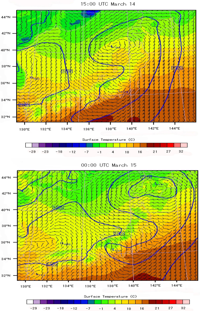
6.3. Local Meteorological Characteristics

Large-scale winds define the general wind regime, and local winds influence the convergence zones. Thus, regional circulation plays an important role in the dispersion of pollutants [94]. Many studies have shown that wind and weather conditions are one of the most important factors determining the formation of photochemical pollution. Other factors include, for example, a stable boundary layer, strong solar radiation, clear sky, weak wind, high temperature, and low humidity. Figure 7 shows the temporal variations of the simulated meteorological conditions throughout the entire domain. In the winter season, the air temperatures were lower, with daily maximum temperatures below 6 °C (Figure 7) in March, and the daily minimum relative humidity was below 75% in general when the photochemical pollution was weak. Figure 7 (15:00 UTC on 14 March) shows the strong winds that occurred at night in the coastal areas of the Sea of Japan. This illustrates that photochemical reactions may have played an important role in the studied episode. It should be noted that the wind speed was relatively strong in the northern part of Japan and that the temperature was lowered due to the influence of the anticyclone, but the ozone peaks were slightly higher in the southern part of Japan (Figure 5). With a view to ascertaining the possible sources of the pollutants that contribute to ozone production, eight back trajectories (Figure 8) were drawn at 6-hour intervals with a time length of 48-hours starting from 00:00 UTC on 16 March 2008 from the EANET monitoring stations in Japan. These back trajectories indicate the air parcels in the east originating from the west and north, where the heavy industrial sources or air pollution sources are located. From this we may presume that the pollutants mainly of mobile origin are responsible for the production of ozone. Figure 7 shows the magnitude of the wind speed and direction based on WRF simulations. The simulated wind direction shows that Japan was under the control of westerly or northwesterly winds from Asia [40].
Figure 7. The temperature distribution (°C) at 15:00 UTC on 14 March and 00:00 UTC on 15 March.
Atmosphere 03 00288 g007
Figure 8. Back trajectories from the observation site drawn at 3-hour intervals starting from 00:00 UTC on 16 March 2008 each with a time length of 48 hours.
Atmosphere 03 00288 g008

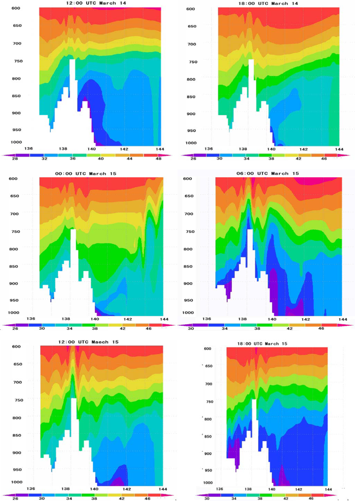
6.4. Vertical Distribution of Ozone Concentrations

This section analyzes the vertical distribution of the ozone concentrations in the PBL and discusses correlations between concentrations in the ground and at elevated levels of the vertical sections of PBL at a fixed latitude (35.7°N) for an east-west cross section of the entire domain from 12:00 UTC on 14 March (9:00 p.m. on 14 March, Japan Standard Time) to 18:00 UTC on 15 March (3:00 a.m. on 16 March, Japan Standard Time). Figure 9 shows the vertical profiles of the mean ozone concentrations in the 3.67 km (600 mbar) layer of the atmosphere based on the WRF/Chem model simulations. The vertical concentrations of ozone were a little higher in the morning and noon than at midnight, while the vertical distribution of tropospheric ozone showed an increase in concentration with height. It is evident that, due to the influence of urbanization in the metropolitan Tokyo area (latitude 35.7°N, longitude 139.7°E), the atmospheric boundary layer becomes stable, and it is thus difficult for ozone to be transported upward and diffused; therefore, the concentration of ozone was lower at the ground level.
In general, the surface ozone exhibits strong diurnal variations, with a mid-afternoon maximum and an early-morning minimum [95,96]. In this study, concentrations of ozone in the ground level during the day were much greater than those at night (Figure 9). At night, the presence of a temperature inversion isolates the surface-level ozone from that of upper levels, as there is little or no vertical mixing between the surface layer and levels above the nocturnal boundary layer (NBL). Surface ozone is partly removed by deposition and reaction with nitric oxide (NO). Because no ozone is produced in the absence of sunlight at night, ozone concentrations begin to decrease after sunset, reaching a minimum in the early morning before sunrise.
After sunrise, the height of the unstable boundary layer begins to increase as the surface is heated and the nocturnal inversion is destroyed. This results in downward mixing of ozone from higher altitudes [97]. Surface ozone is also locally generated by the reactions of nitrogen oxides with volatile organic compounds (VOCs) in the presence of sunlight [22,98,99]. In this study, ozone concentrations increased rapidly from early morning to about noon. Figure 9 shows that the concentration of ozone was 30–34 ppb at ground and level 46 ppb at 3.67 km altitude at 00:00 UTC on 16 March (9:00 a.m. on 15 March, Japan Standard Time). By noon, the mixing height typically exceeded 1 km, and ozone was well mixed within the mixing layer. Strong photochemical production and strong convection in the mid-afternoon period caused ozone concentrations to reach peak values in the late afternoon. In Figure 9, the concentration distribution of ozone was calculated 32–36 in different places at ground level and 50 ppb at 3.67 km altitude at 06:00 UTC on 15 March (15:00 p.m. on 15 March, Japan Standard Time). Ozone production decreased with diminishing sunlight intensity, resulting in a decrease in ozone concentrations with time. At sunset, concentrations decreased substantially below the afternoon maximum value. Figure 9 shows that the ground level ozone concentration at 12:00 UTC on 15 March (9:00 p.m. on 15 March, Japan Standard Time) and 18:00 UTC on 15 March (3:00 a.m. on 16 March, Japan Standard Time) varied from 26–30 ppb. As a new NBL began to form in the evening, ozone concentrations near the surface continued to fall due to surface deposition and reaction with NO. Figure 9 shows that the typical vertical profile of ozone concentrations at night was unbalanced, caused by dry deposition onto the surface and reactions with NO, and that the typical daytime profile was stable, which reflects the important roles of both the local production of ozone and greater convective vertical mixing.
Figure 9. The vertical distribution of ozone concentrations (ppb) in an east-west cross section at a fixed latitude (35.7°N) from 12:00 UTC on 14 March to 18:00 UTC on 15 March (6 hours interval). The y-axis represents the atmospheric pressure (mbar).
Atmosphere 03 00288 g009

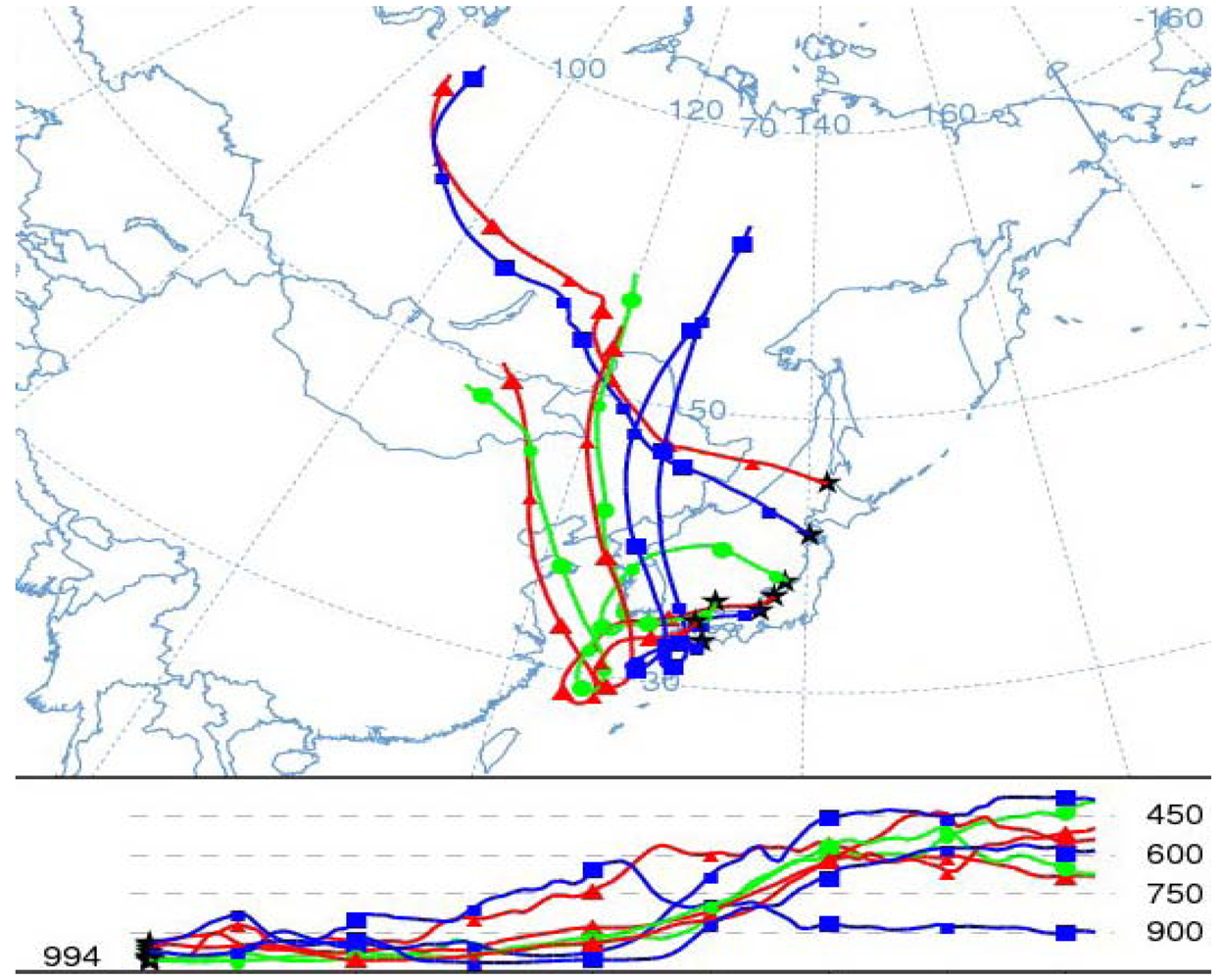
6.5. Tropospheric NOx Transportation

Due to anthropogenic activities, the atmospheric trace gas composition has undergone significant changes during the past few decades. In particular, the tropospheric concentrations of many trace species (e.g., O3, CO, NO, NO2, and CH4) have largely increased. Nitrogen oxides (NOx = NO + NO2) are key species in atmospheric chemistry and are heavily influenced by anthropogenic emissions. The availability of NOx limits photochemical ozone formation in rural and remote regions [22,100] and particularly in the upper troposphere [101], where the impact of ozone on radiative forcing is strongest [102]. NOx also contributes to acid deposition from the atmosphere [103]. While the lifetime of NOx in the atmospheric boundary layer (about a day) is too short to allow transport over large distances, its lifetime in the upper troposphere is of the order of 5–10 days [104], which is sufficient even for intercontinental transport [105]. However, due to removal processes, transport of reactive nitrogen to the upper troposphere is inefficient from the surface, where the largest sources are located [106].
In this study, we simulated the evolution of the NOx plume with the atmospheric chemical transportation model WRF/Chem. The simulation results showed a plume that traveled eastward from east China (06:00 UTC on 14 March) over the East Sea, passing the southern part of the Tohoku region of Japan (00:00 on UTC 15 March) and then floated toward the Pacific Ocean (00:09 UTC on 15 March). Figure 10 shows the NOx concentrations (ppb) over the coastal areas of the Sea of Japan. The pink color in Figure 10 indicates high NOx concentrations (75–80 ppb), which formed in east China and were driven eastward under the influence of strong winds. The average range of NOx concentrations within the entire domain simulated by the WRF/Chem model was 40–60 ppb. Because the photochemical lifetime of NOx depends strongly on the presence of ozone (O3) derived from NOx removal reactions, particularly the conversion ozone to N2O5 via O3 + NO2 → NO3 + O2 and NO2 + NO3 → N2O5 [107], the NOx concentration was approximately 25–30 ppv in the purple area of Figure 10.
Figure 10. NOx concentrations (g/m3) over the coastal areas of the Sea of Japan.
Atmosphere 03 00288 g010

7. Conclusions

By using the new generation of the regional air quality model WRF/Chem V3.3, a two-day heavy-pollution episode in March 2008 was investigated. Rapid ozone changes from 00:00 UTC on 14 March to 00:00 UTC on 16 March were observed throughout the entire domain of the coastal area of the Sea of Japan. During this 2-day period, the daytime and nighttime concentrations of ozone changed from 50 to 30 ppb throughout the entire domain. To understand the processes controlling this rapid change in ozone concentrations, a three-dimensional regional chemical/dynamical model (WRF/Chem) was applied. The results showed that the calculated trends of ozone concentrations and ozone precursors are consistent with the measured trends. The calculated magnitudes and diurnal variations of ozone were slightly underestimated relative to the measured values in most of the rural areas, while they were overestimated in populated urban areas, suggesting that industrial emissions or emissions from biomass burning in populated urban areas are significantly underestimated in this study and that their estimates need to be improved. The model’s relatively coarse horizontal grid spacing in this study may have led to the overestimation in the O3 calculation. Therefore, the resolution of the WRF/Chem model in this study may not be high enough to predict the ozone concentrations over populated Japanese areas. Additionally, because the model is capable of calculating rapid changes in ozone, it is suitable for studying the causes of the changes in ozone. The analysis of the model results suggests that weather conditions play important roles in controlling the surface ozone in the coastal areas of the Sea of Japan. Under the winter weather system, the high ozone concentrations, which were chemically formed in the inland areas, were rapidly transported to the downwind region of the coastal areas, resulting in low ozone concentrations in the urbanized region of East Asia. This study illustrates that the WRF/Chem model is a useful tool for studying the high variability of ozone concentrations. The study of ozone variability has important implications for the prediction of ozone concentrations and for control strategies of high ozone events in the coastal areas of the Sea of Japan.

Acknowledgments

We wish to thank Kobayashi Tomonao of the Faculty of Engineering of Gifu University for sharing resources and data with us. Our deepest gratitude is also expressed to Naher Meherun, the late wife of the first author and a former doctoral student of the Graduate School of Agriculture, Gifu University, who passed away in February 2010.

References

  1. Air Quality in the Mexico Mega City: An Integrated Assessment; Molina, L.; Molina, M. (Eds.) Massachusetts Institute of Technology: Cambridge ,MA, USA, 2002; p. 408.
  2. Paul, R.A.; Biller, W.F.; Mccurdy, T. National Estimates of Population Exposure to Ozone. In Presented at Air Pollution Control Association 80th Annual Meeting and Exhibition, New York, NY, USA, 21–26 June 1987.
  3. Tie, X.; Brasseur, G.; Zhao, C.; Granier, C.; Massie, S.; Qin, Y.; Wang, P.C.; Wang, G.L.; Yang, P.C. Chemical characterization of air pollution in eastern China and the eastern United States. Atmos. Environ. 2006, 40, 2607–2625. [Google Scholar]
  4. Geng, F.H.; Zhao, C.S.; Tang, X.; Lu, G.L.; Tie, X. Analysis of ozone and VOCs measured in Shanghai: A case study. Atmos. Environ. 2007, 41, 989–1001. [Google Scholar] [CrossRef]
  5. Deng, X.J.; Tie, X.; Wu, D.; Zhou, X.J.; Tan, H.B.; Li, F.; Jiang, C. Long-term trend of visibility and its characterizations in the Pearl River Delta Region (PRD), China. Atmos. Environ. 2008, 42, 1424–1435. [Google Scholar]
  6. Zhang, Q.; Zhao, C.; Tie, X.; Wei, Q.; Li, G.; Li, C. Characterizations of aerosols over the Beijing region: A case study of aircraft measurements. Atmos. Environ. 2006, 40, 4513–4527. [Google Scholar]
  7. Sillman, S. The use of NOx, H2O2, and HNO3 as indicators for ozone-NOx-hydrocarbon sensitivity in urban locations. J. Geophys. Res. 1995, 100, 14175–14188. [Google Scholar] [CrossRef]
  8. Kleinman, L.I.; Daum, P.H.; Imre, D.G.; Lee, J.H.; Lee, Y.N.; Nunnermacker, L.J.; Springston, S.R.; Weinstein-Lloyd, J.; Newman, L. Ozone production in the New York City urban plume. J. Geophys. Res. 2000, 105, 14495–14512. [Google Scholar]
  9. Lei, W.; De Foy, B.; Zavala, M.; Volkamer, R.; Molina, L.T. Characterizing ozone production in the Mexico City Metropolitan area, a case study using a chemical transport model. Atmos. Chem. Phys. 2007, 7, 1347–1366. [Google Scholar] [CrossRef]
  10. Zhang, R.; Lei, W.; Tie, X.; Hess, P. Industrial Emissions Cause Extreme Diurnal Urban Ozone Variability. In Proceedings of National Academy Science of the United States of America, Washington, DC, USA, 27 April 2004.
  11. Tie, X.; Madronich, S.; Li, G.H.; Ying, Z.M.; Zhang, R.; Garcia, A.; Lee-Taylor, J.; Liu, Y. Characterizations of chemical oxidants in Mexico City: A regional chemical/dynamical model (WRF/Chem) study. Atmos. Environ. 2007, 41, 1989–2008. [Google Scholar]
  12. Zavala, M.; Lei, W.; Molina, M.J.; Molina, L.T. Modeled and observed ozone sensitivity to mobile-source emissions in Mexico City. Atmos. Chem. Phys. 2009, 9, 39–55. [Google Scholar] [CrossRef] [Green Version]
  13. Geng, F.H.; Qiang, Z.; Tie, X.; Huang, M.; Ma, X.; Deng, Z.; Quan, J.; Zhao, C. Aircraft measurements of O3, NOx, CO, VOCs, and SO2 in the Yangtze River Delta region. Atmos. Environ. 2009, 43, 584–593. [Google Scholar] [CrossRef]
  14. Stephens, S.; Madronich, S.; Wu, F.; Olson, J.B.; Ramos, R.; Retama, A.; Munoz, R. Weekly patterns of Mexico City’s surface concentrations of CO, NOx, PM10 and O3 during 1986-2007. Atmos. Chem. Phys. 2008, 8, 5313–5325. [Google Scholar] [CrossRef]
  15. Ying, Z.M.; Tie, X.; Li, G.H. Sensitivity of ozone concentrations to diurnal variations of surface emissions in Mexico City: A WRF/Chem modeling study. Atmos. Environ. 2009, 43, 851–859. [Google Scholar] [CrossRef]
  16. Kida, M. Countermeasures on Chemical Substances in Japan by Air Pollution Control Law. Available online: http://infofile.pcd.go.th/air/VOC_kida.pdf?CFID=1412050&CFTOKEN=60317530 (accessed on 10 August 2011).
  17. United Nations (UN) Statistics Division. Available online: http://unstats.un.org/unsd/methods/m49/m49regin.htm#asia (accessed on 1 April 2010).
  18. Finlayson-Pitts, B.J.; Pitts, J.N. References. In Chemistry of the Upper and Lower Atmosphere: Theory, Experiments, and Applications; Academic Press: San Diego, CA, USA, 2000. [Google Scholar]
  19. Seinfeld, J.H.; Pandis, S.N. References. In Atmospheric Chemistry and Physics: From Air Pollution to Climate Change; John Wiley & Sons: New York, NY, USA, 1998. [Google Scholar]
  20. Thielmann, A.; Prevot, A.S.H.; Staehelin, J. Sensitivity of ozone production derived from field measurements in the Italian Po basin. J. Geophys. Res. 2002, 107. [Google Scholar] [CrossRef]
  21. Altshuller, A.P.; Lefohn, A.S. Background ozone in the planetary boundary layer over the United States. J. Air Waste Manag. Assoc. 1996, 46, 134–141. [Google Scholar] [CrossRef]
  22. Chameides, W.L.; Fehsenfeld, F.; Rodgers, M.O.; Cardelino, C.; Martinez, J.; Parrish, D.; Lonneman, W.; Lawson, D.R.; Rasmussen, R.A.; Zimmerman, P.; Greenberg, J.; Mlddleton, P.; Wang, T. Ozone precursor relationships in the ambient atmosphere. J. Geophys. Res. 1992, 97, 6037–6055. [Google Scholar]
  23. National Research Council (NRC), References. In Rethinking the Ozone Problem in Urban and Regional Air Pollution; National Academy Press: Washington, DC, USA, 1991.
  24. U.S. Environmental Protection Agency (U.S. EPA). Technology Transfer Network OAR Policy and Guidance. Available online: http://www.epa.gov/ttn/oarpg/t1/fr_notices/3866finalfrnotice.pdf (accessed on 25 March 2005).
  25. Skamarock, W.C.; Klemp, J.B.; Dudhia, J.; Gill, D.O.; Barker, D.M.; Wang, W.; Powers, J.G. A Description of the Advanced Research WRF Version 2; TN-468tSTR; NCAR Technical note. NCAR: Boulder, CO, USA, 2005; 88. [Google Scholar]
  26. Grell, G.A.; Peckham, S.E.; Schmitz, R.; McKeen, S.A.; Frost, G.; Skamarock, W.; Eder, B. Fully coupled “online” chemistry within the WRF model. Atmos. Environ. 2005, 39, 6957–6975. [Google Scholar]
  27. Byun, D.W.; Ching, J.K.S. Science algorithms of the EPA Models-3 Community Multiscale Air Quality Model (CMAQ) Modeling System; EPA/600/R-99/030. US Environmental Protection Agency, Office of Research and Development: Washington, DC, USA, 1999. [Google Scholar]
  28. Sistla, G.; Zhou, N.; Hao, W.; Ku, J.Y.; Rao, S.T.; Bornstein, R.; Freedman, F.; Thunis, P. Effects of uncertainties in meteorological inputs on urban airshed model predictions and ozone control strategies. Atmos. Environ. 1996, 30, 2011–2025. [Google Scholar] [CrossRef]
  29. Jimenez, P.; Jorba, O.; Parra, R.; Baldasano, J.M. Evaluation of MM5-EMICAT2000-CMAQ performance and sensitivity in complex terrain: High resolution application to the northeastern Iberian Peninsula. Atmos. Environ. 2006, 40, 5056–5072. [Google Scholar] [CrossRef]
  30. Mao, Q.; Gautney, L.L.; Cook, T.M.; Jacobs, M.E.; Smith, S.N.; Kelsoe, J.J. Numerical experiments on MM5-CMAQ sensitivity to various PBL schemes. Atmos. Environ. 2006, 30, 3092–3110. [Google Scholar]
  31. Zhang, Y.; Liu, P.; Pun, B.; Seigneur, C. A comprehensive performance evaluation of MM5-CMAQ for the summer 1999 southern oxidants study episode—Part I: Evaluation protocols, databases, and meteorological predictions. Atmos. Environ. 2006, 40, 4825–4838. [Google Scholar] [CrossRef]
  32. Otte, T.L. The impact of nudging in the meteorological model for retrospective air quality simulations. Part I: Evaluation against national observation networks. J. Appl. Meteorol. Climat. 2008, 47, 1853–1867. [Google Scholar] [CrossRef]
  33. Zhang, Y.; Hu, X.M.; Howell, G.W.; Sills, E.; Fast, J.D.; Gustafson, W.I.; Zaveri, R.A.; Grell, G.A.; Peckham, S.E.; McKeen, S.A. Modeling Atmospheric Aerosols in WRF/Chem. In Proceedings of 6th/15th MM5 Users’ Workshop, Boulder, CO, USA, 27-30 June 2005.
  34. Fast, J.D.; Gustafson, W.I.; Easter, R.C.; Zaveri, R.A.; Barnard, J.C.; Chapman, E.G.; Grell, G.A.; Peckham, S.E. Evolution of ozone, particulates, and aerosol direct radiative forcing in the vicinity of Houston using a fully coupled meteorology chemistry aerosol model. J. Geophys. Res. Atmos. 2006, 111. [Google Scholar] [CrossRef]
  35. Misenis, C.; Hu, X.M.; Krishnan, S.; Zhang, Y.; Fast, J.D. Sensitivity of WRF/Chem Predictions to Meteorological Schemes. In Proceedings of the 86th Annual AMS Annual Meeting, 14th Joint Conference on the Applications of Air Pollution Meteorology with the Air and Waste Management Associated, Atlanta, GA, USA, 27 January-3 February; 2006. [Google Scholar]
  36. Jiang, F.; Wang, T.J.; Wang, T.T.; Xie, M.; Zhao, H. Numerical modeling of a continuous photochemical pollution episode in Hong Kong using WRF-CHEM. Atmos. Environ. 2008, 42, 8717–8727. [Google Scholar] [CrossRef]
  37. De Foy, B.; Fast, J.D.; Paech, S.J.; Phillips, D.; Walters, J.T.; Coulter, R.L.; Martin, T.J.; Pekour, M.S.; Shaw, W.J.; Kastendeuch, P.P.; Marley, N.A.; Retama, A.; Molina, L.T. Basin scale wind transports during the MILAGRO field campaign and comparison to climatology using cluster analysis. Atmos. Chem. Phys. 2008, 8, 1209–1224. [Google Scholar]
  38. Tie, X.; Madronich, S.; Li, G.; Ying, Z.; Weinheimer, A.; Apel, E.; Campos, T. Simulation of Mexico City plumes during the MIRAGE-Mex field campaign using the WRF-Chem model. Atmos. Chem. Phys. 2009, 9, 4621–4638. [Google Scholar] [CrossRef]
  39. Zhang, Y.; Dubey, M.K.; Olsen, S.C.; Zheng, J.; Zhang, R. Comparisons of WRF/Chem simulations in Mexico City with ground-based RAMA measurements during the 2006-MILAGRO. Atmos. Chem. Phys. 2009, 9, 3777–3798. [Google Scholar] [CrossRef]
  40. Chatani, S.; Sudo, K. Influences of the variation in inflow to East Asia on surface ozone over Japan during 1996-2005. Atmos. Chem. Phys. 2011, 11, 8745–8758. [Google Scholar] [CrossRef]
  41. Masanori, N.; Masayuki, T.; Hajime, A.; Masahisa, N.; Tomohiro, N.; Tetsu, S.; Yuzo, M. Evaluation of vertical ozone profiles simulated by WRF/Chem using lidar-observed data. SOLA 2007, 3, 133–136. [Google Scholar] [CrossRef]
  42. Kurokawa, J.; Ohara, T.; Uno, I.; Hayasaki, M.; Tanimoto, H. Influence of meteorological variability on interannual variations of the springtime boundary layer ozone over Japan during 1981-2005. Atmos. Chem. Phys. 2009, 9, 6287–6304. [Google Scholar] [CrossRef]
  43. Kurokawa, J.; Ohara, T.; Uno, I.; Hayasaki, M. Analysis of episodic pollution of photochemical ozone during 8-9 May 2007 over Japan using the nesting RAMS/CMAQ modeling system. J. Japan Soc. Atmos. Environ. 2008, 43, 209–224. [Google Scholar]
  44. Hayasaki, M.; Ohara, T.; Kurokawa, J.; Uno, I.; Shimizu, A. Episodic pollution of photochemical ozone during 8-9 May 2007 over Japan: Observational data analysis. J. Japan Soc. Atmos. Environ. 2008, 43, 225–237. (in Japanese).. [Google Scholar]
  45. Saikawa, E.; Kurokawa, J.; Takigawa, M.; Mauzerall, D. L.; Horowitz, L. W.; Ohara, T. The impact of China’s vehicle emissions on regional air quality in 2000 and 2020: A scenario analysis. Atmos. Chem. Phys. Discuss. 2011, 11, 13141–13192. [Google Scholar] [CrossRef]
  46. Wesley, M.L. Parameterization of surface resistance to gaseous dry deposition in regional numerical models. Atmos. Environ. 1989, 16, 1293–1304. [Google Scholar]
  47. Madronich, S.; Flocke, S. References. In The Handbook of Environmental Chemistry; Springer-Verlag: Heidelberg, Berlin, Germany, 1999; pp. 1–26. [Google Scholar]
  48. Tie, X.; Madronich, S.; Walters, S.; Zhang, R.; Rasch, P.; Collins, W. Effect of clouds on photolysis and oxidants in the troposphere. J. Geophys. Res. 2003, 108. [Google Scholar] [CrossRef]
  49. Chang, J.S.; Middleton, P.B.; Stockwell, W.R.; Walcek, C.J.; Pleim, J.E.; Lansford, H.H.; Madronich, S.; Binkowski, F.S.; Seaman, N.L.; Stauffer, D.R. The Regional Acid Deposition Model and Engineering Model; Report No. 4; NAPAP SOS/T: Washington, DC, USA, 1989. [Google Scholar]
  50. Schell, B.; Ackermann, I.J.; Hass, H.; Binkowski, F.S.; Ebel, A. Modeling the formation of secondary organic aerosol within a comprehensive air quality model system. J. Geophys. Res. 2001, 106, 28275–28293. [Google Scholar]
  51. S Korea Bid to Solve Sea Dispute. BBC News. 2007. Available online: http://news.bbc.co.uk/2/hi/asia-pacific/6240051.stm (accessed on 8 January 2007).
  52. The Ministry of Foreign Affairs and Trade, Republic of Korea (MFAT). Report on the Progress in Consultations on the Naming of the Sea Area between the Korean Peninsula and the Japanese Archipelago. In Proceedings of Ninth United Nations Conference on the Standardization of Geographical Names, 21-30 August 2007; E/CONF.98/CRP.81.. United Nations Economic and Social Council: New York, NY, USA.
  53. David, W.A.; Ashby, N.; Hodge, C.C. The Science of Timekeeping. Hewlett-Packard; Application Note No. 1289. Allan’s Time Interval Metrology Enterprise: Fountain Green, UT, USA, 1997. [Google Scholar]
  54. Hanado, Y.; Imamura, K.; Kotake, N.; Nakagawa, F.; Shimizu, Y.; Tabuchi, R.; Takahashi, Y.; Hosokawa, M.; Morikawa, T. The new generation system of Japan standard time at NICT. Int. J. Nav. Observ. 2008. [Google Scholar] [CrossRef]
  55. Binkowski, F.S.; Shankar, U. The regional particulate matter model, 1. Mode description and preliminary results. J. Geophys. Res. 1995, 100, 26191–26209. [Google Scholar] [CrossRef]
  56. Hong, S.Y.; Dudhia, J.; Chen, S.H. A revised approach to ice microphysical processes for the bulk parameterization of clouds and precipitation. J. Amer. Met. Soc. 2004, 132, 103–120. [Google Scholar]
  57. Ahmad, N.; Linderman, J. A godunov-type finite volume scheme for meso- and micro-scale flows in three dimensions. Pure Appl. Geophys. 2008, 165, 1929–1939. [Google Scholar] [CrossRef]
  58. Baldauf, M.; Skamarock, W.C. An Improved Third Order Vertical Advection Scheme for the Runge-Kutta Dynamical Core. In Proceedings of8th International SRNWP-Workshop on Non-Hydrostatic Modelling, Bad Orb, Germany, 26-28 October 2009.
  59. Mlawer, E.J.; Taubman, S.J.; Brown, P.D.; Iacono, M.J.; Clough, S.A. Radiative transfer for inhomogeneous atmosphere: RRTM, a validated correlated-k model for the long wave. J. Geophys. Res. 1997, 102, 16663–16682. [Google Scholar]
  60. Shin, H.H.; Hong, S.-Y.; Dudhia, J.; Kim, Y.-J. Orography-induced gravity wave drag parameterization in the global WRF: Implementation and sensitivity to shortwave radiation schemes. Adv. Meteorol. 2010, 2010. [Google Scholar] [CrossRef]
  61. Dudhia, J. Numerical study of convection observed during the winter monsoon experiment using a mesoscale two-dimensional model. J. Atmos. Sci. 1989, 46, 3077–3107. [Google Scholar] [CrossRef]
  62. Monin, A.S.; Obukhov, A.M. Basic laws of turbulent mixing in the surface layer of the atmosphere. Contrib. Geophys. Inst. Slov. Acad. Sci. 1954, 151, 163–187. (in Russian).. [Google Scholar]
  63. Ek, M.B.; Mitchell, K.E.; Lin, Y.; Rogers, E.; Grunmann, P.; Koren, V.; Gayno, G.; Tarpley, J.D. Implementation of Noah land surface model advances in the National Centers for Environmental Prediction operational mesoscale Eta model. J. Geophys. Res. 2003, 108, 8851–8867. [Google Scholar]
  64. Janjic, Z.I. The step-mountain coordinate: Physical package. Mon. Wea. Rev. 1990, 118, 1429–1443. [Google Scholar] [CrossRef]
  65. Janjic, Z.I. The step-mountain ETA coordinate model: Further development of the convection, viscous sub-layer, and turbulent closure schemes. Mon. Wea. Rev. 1994, 122, 927–945. [Google Scholar] [CrossRef]
  66. Grell, G.A.; Devenyi, D. A generalized approach to parameterizing convection combining ensemble and data assimilation techniques. Geophys. Res. Lett. 2002, 29. [Google Scholar] [CrossRef]
  67. Stockwell, W.R.; Middleton, P.; Chang, J.S. The second generation regional acid deposition model chemical mechanism for regional air quality modeling. J. Geophys. Res. 1990, 95, 16343–16367. [Google Scholar] [CrossRef]
  68. Wesley, M.L. Parameterization of surface resistance to gaseous dry deposition in regional numerical models. Atmos. Environ. 1989, 16, 1293–1304. [Google Scholar]
  69. Guenther, A.B.; Zimmerman, P.R.; Harley, P.C.; Monson, R.K.; Fall, R. Isoprene and monoterpene emission rate variability: Model evaluations and sensitivity analyses. J. Geophys. Res. Atmos. 1993, 98, 12609–12617. [Google Scholar]
  70. Guenther, A.; Zimmerman, P.; Wildermuth, M. Natural volatile organic compound emission rate estimates for US woodland landscapes. Atmos. Environ. 1994, 28, 1197–1210. [Google Scholar] [CrossRef]
  71. Madronich, S. Photodissociation in the atmosphere 1. Actinic flux and the effects of ground reflections and clouds. J. Geophys. Res. 1987, 92, 9740–9752. [Google Scholar] [CrossRef]
  72. Schell, B.; Ackermann, I.J.; Hass, H.; Binkowski, F.S.; Ebel, A. Modeling the formation of secondary organic aerosol within a comprehensive air quality model system. J. Geophys. Res. 2001, 106, 28275–28293. [Google Scholar]
  73. Freitas, S.R.; Longo, K.; Silva Dias, M.; Silva Dias, P.; Chatfield, R.; Prins, E.; Artaxo, P.; Grell, Y.G.; Recuero, F. Monitoring the transport of biomass burning emissions in South America. Environ. Fluid Mech. 2005, 5, 135–167. [Google Scholar] [CrossRef]
  74. Longo, K.; Freitas, S. R.; Setzer, A.; Prins, E.; Artaxo, P.; Andreae, M. The coupled aerosol and tracer transport model to the Brazilian developments on the regional atmospheric modeling system (CATT-BRAMS). Part 2: Model sensitivity to the biomass burning inventories. Atmos. Chem. Phys. Discuss. 2007, 8571–8595.
  75. Granier, C.; Niemeir, U.; Muller, J. F.; Olivier, J.; Peters, J.; Richter, A.; Nuss, H.; Burrows, J. Variation of the Atmospheric Composition over the 1990-2000 Period; EU project EVK2-1999-00011, Report No. 6. POET: Paris, France, 2003. [Google Scholar]
  76. Olivier, J.; Peters, J.; Granier, C.; Petron, G.; Muller, J.F.; Wallens, S. Present and Future Surface Emissions of Atmospheric Compounds; EU project EVK2-1999-00011, POET report No. 2. POET POET: Paris, France, 2003. [Google Scholar]
  77. Schultz, M. RETRO team. RETRO Emission Trends and Variability. Presented at 1st ACCENT Symposium, Urbino, Italy, 12–16 September 2005; 2005. Available online: http://retro.enes.org/index.shtml (accessed on 8 April 2008).
  78. Olivier, J.G.J.; Bouwman, A.F.; Van der Maas, C.W.M.; Berdowski, J.J.M.; Veldt, C.; Bloos, J.P.J.; Visschedijk, A.J.H.; Zandveld, P.Y.J.; Haverlag, J.L. Description Of EDGAR Version 2.0: A Set of Global Emission Inventories of Greenhouse Gases and Ozone-Depleting Substances for All Anthropogenic and Mos-Natural Sources on a Per Country Basis and On a 1 × 1 Grid; RIVM report No. 771060 002. RIVM: Bilthoven, The Netherlands, 1996. Available online: http://www.mnp.nl/edgar/introduction (accessed on 5 October 2010).
  79. Olivier, J.G.J.; Bloos, J.P.J.; Berdowski, J.J.M.; Visschedijk, A.J.H.; Bouwman, A.F. A 1990 global emission inventory of anthropogenic sources of carbon monoxide on 1 × 1 developed in the framework of EDGAR/GEIA. Chemosphere: Global Change Sci. 1999, 1, 1–17. [Google Scholar] [CrossRef]
  80. Olivier, J.G.J.; Berdowski, J.J.M.; Peters, J.A.H.W.; Bakker, J.; Visschedijk, A.J.H.; Bloos, J.-P.J. Applications of EDGAR. Including a Description of EDGAR 3.0: Reference Database with Trend Data for 1970-1995; Bilthoven; RIVM report no. 773301 001/ NOP report no. 410200 051. RIVM: Bilthoven, The Netherlands, 2001. [Google Scholar]
  81. Van der Werf, G.R.; Randerson, J.T.; Collatz, G.J.; Giglio, L.; Kasibhatla, P.S.; Avelino, A.; Olsen, S.C.; Kasischke, E.S. Continental-scale partitioning of fire emissions during the 1997-2001 El Nino/La Nina period. Science. 2004, 303. Available online: http://daac.ornl.gov/VEGETATION/guides/global_fire_emissions_v2.1.html. (accessed on 22 June 2010).
  82. Van der Werf, G.R.; Randerson, J.T.; Giglio, L.; Collatz, G.J.; Kasibhatla, P.S. Interannual variability in global biomass burning emission from 1997 to 2004. Atmos. Chem. Phys. 2006, 6, 3423–3441. [Google Scholar] [CrossRef]
  83. Andres, R.J.; Fielding, D.J.; Marland, G.; Boden, T.A.; Kumar, N. Carbon dioxide emissions from fossil-fuel use 1751-1950. Tellus 1999, 51, 759–765. [Google Scholar]
  84. Saiki, M. Annual Report on Atmospheric and Marine Environment Monitoring: Observation Results for 2008; No. 10. Global Environment and Marine Department,Japan Meteorological Agency (JMA): Tokyo, Japan, 2010. [Google Scholar]
  85. Segami, A. Annual Report on Atmospheric and Marine Environment Monitoring: Observation result for 2009; No. 11. Global Environment and Marine Department,Japan Meteorological Agency (JMA): Tokyo, Japan, 2011. [Google Scholar]
  86. National Institute for Environmental Studies. Observation Data Download for Pollutant Concentration in the Atmospheric Environment. Available online: http://www.nies.go.jp/igreen/td_down.html (accessed on 20 July 2010) (in Japanese).
  87. Ministry of the Environment (MOE). The Status of Atmosphere Pollution. Available online: http://www.env.go.jp/air/osen/index.html (accessed on 20 August 2010) (in Japanese).
  88. Simpson, D.; Olendrzynacuteski, K.; Semb, A.; Storen, E.; Unger, S. Photochemical Oxidant Modeling In Europe: Multi-Annual Modeling and Source Receptor Relationships; EMEP MSC-W Report 3/97. Norwegian Meteorological Institute: Oslo, Norway, 1997. [Google Scholar]
  89. Giorgi, F.; Meleux, F. Modelling the regional effects of climate change on air quality. C. R. Geosci. 2007, 339, 721–733. [Google Scholar] [CrossRef]
  90. Hirofumi, A. Air Pollution Control Policy in Japan for Mitigating Sulphur Emission. In Presentation of the International Conference on Transboundary Air Pollution in North-East Asia, Tokyo, Japan, 17–19 December 2008.
  91. Val, B. Cyclones and Anticyclones in the Mid-Latitudes. Available online: www.aos.wisc.edu/~aos101vb/val_cyclones.ppt (accessed on 2 January 2010).
  92. National Weather Service. Available online: http://www.srh.weather.gov/srh/jetstream/index.htm (accessed on 24 October 2006).
  93. Vautard, R.; Honore, C.; Beekmanna, M.; Rouil, L. Simulation of ozone during the August 2003 heat wave and emission control scenarios. Atmos. Environ. 2005, 39, 2957–2967. [Google Scholar] [CrossRef]
  94. Seaman, N.L. Meteorological modeling for air-quality assessments. Atmos. Environ. 2000, 34, 2231–2259. [Google Scholar] [CrossRef]
  95. Logan, J.A. Ozone in rural areas of the United States. J. Geophys. Res. 1989, 94, 8511–8532. [Google Scholar] [CrossRef]
  96. Parrish, D.D.; Buhr, M.P.; Trainer, M.; Norton, R.B.; Shimshock, J.P.; Fehsenfeld, C.F.; Anlauf, K.G.; Bottenheim, J.W.; Tang, Y.Z.; Wiebe, H.A.; Roberts, J.M.; Tanner, R.L.; Newman, L.; Bowersox, V.C.; Olszyna, K.J.; Bailey, E.M.; Rodgers, M.O.; Wang, T.; Berresheim, H.; Roychowdhury, U.K.; Demerjiani, K.L. The total oxidized nitrogen levels and the partitioning between the individual species at six rural sites in eastern North America. J. Geophys. Res. 1993, 98, 2927–2939. [Google Scholar]
  97. Trainer, M.; Williams, E.J.; Parrish, D.D.; Buhr, M.P.; Allwine, E.J.; Westberg, H.H.; Fehsenfeld, F.C.; Liu, S.C. Models and observations of the impact of natural hydrocarbons on rural ozone. Nature 1987, 329, 705–707. [Google Scholar] [CrossRef]
  98. Warneck, P. Chemistry of the Natural Atmosphere; Academic Press Inc.: London, UK, 1988. [Google Scholar]
  99. National Research Council (NRC), References. In Rethinking the Ozone Problem in Urban and Regional Air Pollution; National Academy Press: Washington, DC, USA, 1992.
  100. Lin, X.; Trainer, M.; Liu, S.C. On the nonlinearity of the tropospheric ozone production. J. Geophys. Res. 1988, 93, 15879–15888. [Google Scholar]
  101. Levy, H.; Moxim, W.J.; Klonecki, A.A.; Kasibhatla, P.S. Simulated tropospheric NOx: Its evaluation, global distribution and individual source contributions. J. Geophys. Res. 1999, 104, 26279–26306. [Google Scholar]
  102. Johnson, C.; Henshaw, J.; McInnes, G. Impact of aircraft and surface emissions of nitrogen oxides on tropospheric ozone and global warming. Nature 1992, 355, 69–71. [Google Scholar]
  103. Stoddard, J.L.; Jeffries, D.S.; Lukeville, A.; Clair, T.A.; Dillon, P.J.; Driscoll, C.T.; Forsius, M.; Johannessen, M.; Kahl, J.S.; Kellogget, J.H.; et al. Regional trends in aquatic recovery from acidification in North America and Europe. Nature 1999, 401, 575–578. [Google Scholar]
  104. Stoddard, J.L.; Jeffries, D.S.; Lükewille, A.; Clair, T.A.; Dillon, P.J.; Driscoll, C.T.; Forsius, M.; Johannessen, M.; Kahl, J.S.; Kellogg, J.H.; et al. Sources and chemistry of NOx in the upper troposphere over the United States. Geophys. Res. Lett. 1998, 25, 1705–1708. [Google Scholar]
  105. Stohl, A.; Eckhardt, S.; Forster, C.; James, P.; Spichtinger, N. On the pathways and timescales of intercontinental air pollution transport. J. Geophys. Res. 2002, 107. [Google Scholar] [CrossRef]
  106. Murphy, D.; Fahey, D.; Profitt, M.; Liu, S.; Chan, K.; Eubank, C.; Kawa, S.; Kelly, K. Reactive nitrogen and its correlation with ozone in the lower stratosphere and upper troposphere. J. Geophys. Res. 1993, 98, 8751–8773. [Google Scholar]
  107. Von Kuhlmann, R.; Lawrence, M.G.; Crutzen, P.J.; Rasch, P.J. A model for studies of tropospheric ozone and nonmethane hydrocarbons: Model description and ozone results. J. Geophys. Res. 2003, 108. [Google Scholar] [CrossRef]

