Machine Learning-Based Reconstruction of Missing Meteorological Observations Using Reanalysis and Satellite Data in West Africa

Abstract

High-frequency meteorological observations from automatic weather stations (AWS) are frequently affected by substantial data gaps in data-sparse regions such as West Africa, limiting their usability for climate analysis and decision-making. This study presents a machine learning-based framework for reconstructing missing hourly observations by integrating in situ AWS measurements with ERA5-Land reanalysis fields and Global Precipitation Measurement (GPM) satellite-derived products. The framework was applied to a network of over 50 AWS across 10 West African countries over the period 2017–2025, targeting seven meteorological variables: air temperature, relative humidity, global solar radiation, atmospheric pressure, precipitation, wind speed, and wind direction. Gradient boosting models (XGBoost, LightGBM, and CatBoost) were trained following a station-wise and variable-wise strategy, yielding over 300 variable-specific models. Detailed quantitative results are reported for four representative stations spanning distinct agro-climatic zones (Sahelian, Sudanian, coastal, and humid tropical). Air temperature and atmospheric pressure exhibit the highest reconstruction skill, with R² values typically exceeding 0.90, while relative humidity and global solar radiation achieve R² between 0.80 and 0.92. Precipitation and wind speed showed lower reconstruction skill than thermodynamic variables, reflecting their intermittency and sensitivity to local-scale processes. Wind direction, evaluated separately using circular statistics after recombination into degrees, exhibited the largest angular errors, highlighting the difficulty of reconstructing directional variability from large-scale predictors alone.

1. Introduction

High-quality in situ meteorological observations are fundamental to climate monitoring, climate services, and evidence-based decision-making in sectors such as agriculture, water resources, disaster risk reduction, and energy planning. In West Africa, where climate variability and extremes strongly influence socio-economic systems, the availability of reliable and continuous observational data is particularly critical [1,2].

The West African Science Service Centre on Climate Change and Adapted Land Use (WASCAL) operates a regional network of over 50 automatic weather stations (AWS) distributed across ten West African countries. These stations provide high-frequency observations of key atmospheric variables. However, as is common in data-sparse regions, the resulting time series are affected by frequent gaps caused by sensor malfunctions, battery failures, limited maintenance capacity, vandalism, and intermittent data transmission [3]. Such gaps significantly limit the usability of the datasets for climate analysis, trend estimation, and model evaluation.

Conventional gap-filling approaches, including interpolation, climatological substitution, and direct use of reanalysis data, are straightforward to implement but often fail to capture local variability and extreme events [4,5], with downstream consequences for trend estimation [6]. Statistical interpolation methods such as linear and spline interpolation are effective for short gaps in smoothly varying variables but degrade for longer gaps or highly intermittent processes such as precipitation [5]. Climatological approaches tend to smooth temporal variability and fail to reproduce extremes, which can introduce biases in climate analyses [5,7]. Reanalysis datasets such as ERA5-Land provide spatially complete fields frequently used to fill observational gaps; however, they suffer from scale mismatch and systematic biases at the station level [8]. Satellite products such as those derived from the Global Precipitation Measurement (GPM) mission offer complementary skill for rainfall occurrence detection in convective regimes, despite persistent magnitude biases [7].

Table 1. Summary of relative merits and limitations of key studies on meteorological data gap filling referenced in this work.

Ref.	Method/Focus	Region & Variable(s)	Key Merit	Key Limitation
[3]	Comparative evaluation of imputation methods	Burkina Faso & Senegal; multiple variables	Region-specific West African benchmark of imputation performance	Conventional/statistical methods only; no multi-source ML integration
[4]	Gap filling of monthly temperature data	Global; temperature, monthly	Quantifies impact of gap-filling choice on trend estimation	Coarse monthly resolution; single variable
[5]	Review of climate time-series imputation methods	General review; multiple variables	Broad synthesis of imputation techniques and their applicability	Conventional methods reviewed degrade for long gaps and intermittent variables
[7]	Gap-filled daily rainfall with uncertainty quantification	Hawai’i; rainfall, daily	Explicit uncertainty characterization of gap-filled values	Single-variable, daily resolution; no multi-source ML
[6]	Impact of gap filling on precipitation trend estimation	Morocco (Souss Massa); precipitation	Evaluates downstream impact of gap-filling method on trends	Basin-specific, single-variable focus
[8]	ERA5 global reanalysis (data source)	Global; all variables, hourly grid	Spatially complete, widely used reference dataset	~9 km scale mismatch and systematic bias at station level
[9]	Debiased ERA5 substitution for gap filling	Regional; temperature, hourly	Shows bias correction of reanalysis reduces substitution error	Single-variable (temperature) focus
[10]	Comparative analysis of ML gap-filling approaches	Multiple variables, general	Demonstrates ML outperforms traditional techniques	Not evaluated in West African/tropical convective context
[11]	ClimateFiller: AI + multi-source reanalysis framework	General; multiple variables	Combines AI with multi-source reanalysis, conceptually closest to this study	Not benchmarked at hourly resolution across a dense regional AWS network

summarizes the relative merits and limitations of the main studies on meteorological gap filling referenced above, providing a structured comparison of their scope, strengths, and constraints.

Recent advances in machine learning offer promising alternatives by exploiting nonlinear relationships between in situ observations and auxiliary data sources. Tree-based ensemble models, particularly gradient boosting approaches, have demonstrated improved performance compared to traditional techniques across multiple meteorological variables when physically consistent large-scale predictors are available [3,5,10]. Hybrid frameworks integrating multi-source reanalysis data with machine learning have further shown improved reconstruction performance at sub-daily time scales [5,7,11]. Despite these advances, most existing studies focus on daily or monthly resolutions and a limited number of variables, leaving high-frequency multi-variable reconstruction in data-sparse tropical regions comparatively underexplored.

This study proposes a machine learning-based framework for reconstructing missing hourly AWS observations across West Africa by combining station data with ERA5-Land reanalysis and GPM satellite products. The main contributions are: (i) a station-wise and variable-wise gap-filling framework accounting for local climatic characteristics; (ii) a comparative evaluation of XGBoost, LightGBM, and CatBoost against a reanalysis-based baseline across seven meteorological variables; and (iii) an assessment of reconstruction performance across stations from contrasting climatic contexts. Results demonstrate that gradient boosting models substantially outperform both linear interpolation and direct ERA5-Land substitution, with CatBoost achieving R² above 0.90 for temperature and pressure, and meaningful improvements across all variables. The remainder of this paper is organized as follows: Section 2 describes the materials and methods. Section 3 reports the results. Section 4 discusses the findings, and Section 5 presents the conclusions.

2. Materials and Methods

This section describes the data sources, preprocessing procedures, feature engineering strategy, machine learning modeling approach, and reconstruction protocol used to develop the gap-filling framework. The overall workflow integrates in situ AWS observations with reanalysis and satellite-derived auxiliary data through a station-wise and variable-wise supervised learning pipeline.

2.1. Overview of the Gap-Filling Framework

The proposed framework aims to reconstruct continuous hourly meteorological time series from incomplete AWS observations by leveraging reanalysis and satellite-derived information through supervised machine learning. The approach follows a station-wise and variable-wise strategy, in which independent models are developed for each target variable at each station. This design allows the framework to explicitly account for local climatic characteristics, variable-level data availability, and variable-specific physical processes.

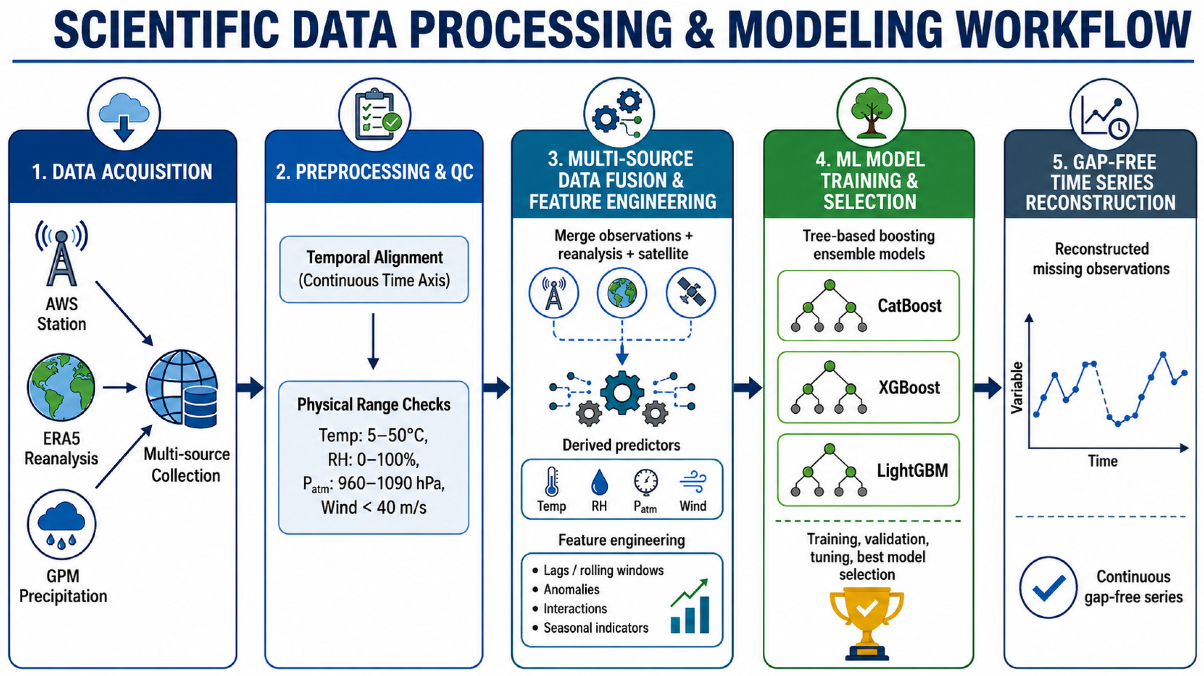
The overall workflow consists of five main steps (Figure 1): (i) acquisition and harmonization of in situ AWS observations and auxiliary data sources, (ii) preprocessing and quality control of station observations, (iii) multi-source data fusion and feature engineering, (iv) machine learning model training and selection, and (v) reconstruction of gap-free time series with physical post-processing constraints.

All data processing, model training, and figure generation were performed using Python (version 3.11.5), leveraging libraries including NumPy (version 1.26.4), Pandas (version 2.2.3), Scikit-learn (version 1.4.2), XGBoost (version 2.1.3), LightGBM (version 4.4.0), CatBoost (version 1.2.7), Optuna (version 4.3.0), Matplotlib (version 3.9.2), and Seaborn (version 0.13.2). For selected figures, titles and graphical annotations were subsequently added using Canva (Canva Pty Ltd., Sydney, Australia).

2.2. Study Area and In Situ Data

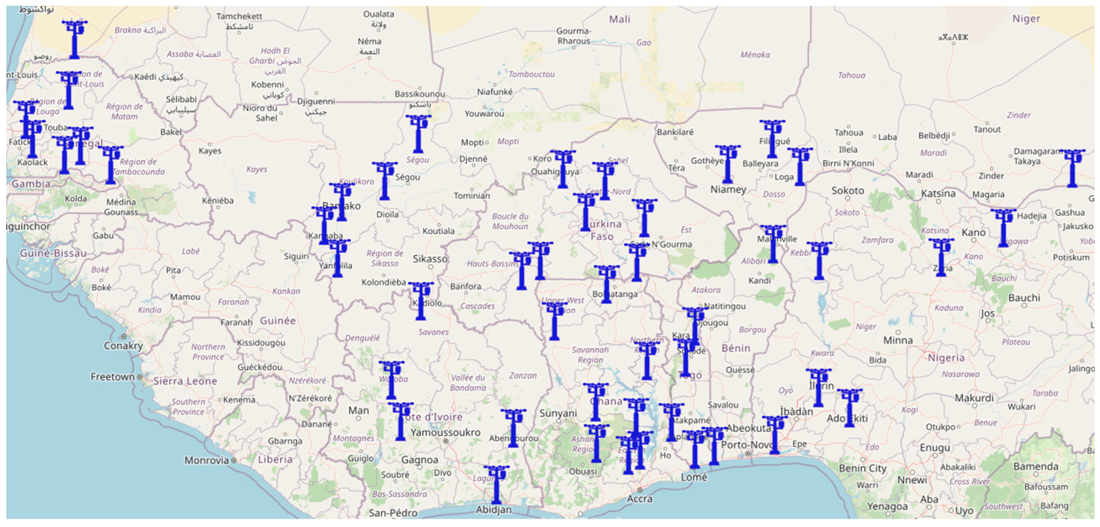
The WASCAL regional AWS network covers a wide range of climatic regimes, from the Sahelian zone in the north to the coastal and humid regions in the south (Figure 2). The network comprises over 50 stations distributed across ten West African countries: Benin, Burkina Faso, Côte d’Ivoire, Ghana, Mali, Niger, Nigeria, Senegal, The Gambia, and Togo. Observations span the period 2017–2025 and are originally recorded at a 10 min temporal resolution. For most variables, the AWS provide minimum, maximum, and mean values over the recording interval, while precipitation is recorded as a single accumulated value. The WASCAL AWS used in this study are NESA automatic weather stations equipped with Evolution data loggers (NESA Srl, Vidor, Italy). The stations use a standardized set of meteorological sensors to measure the seven variables considered in this study. Air temperature and relative humidity are measured using the UTA combined thermo-hygrometric sensor, atmospheric pressure is recorded by the e-Bar piezoresistive barometer integrated into the Evolution data logger, precipitation is measured using the PL400 tipping-bucket rain gauge, global solar radiation is measured using the RSG2Std Class A pyranometer, and wind speed and direction are measured using the ANESR biaxial ultrasonic anemometer. The corresponding manufacturer-specified measurement accuracies are summarized in

Table 2. Instrumentation and manufacturer-specified measurement accuracy of the NESA automatic weather stations used in the WASCAL network.

Meteorological Variable	NESA Sensor	Sensor Type	Manufacturer-Specified Accuracy
Air temperature	UTA	Pt100 1/3 DIN combined thermo-hygrometric sensor	±0.1 °C at 0 °C; <0.3 °C full scale
Relative humidity	UTA	Capacitive humidity sensor combined with air temperature	±1% RH FS at 23 °C
Atmospheric pressure	e-Bar	Piezoresistive barometer integrated into the Evolution data logger	±0.4 hPa at 20 °C
Precipitation	PL400	Tipping-bucket rain gauge	±2%; ±1% on request
Global solar radiation	RSG2Std	Double-thermopile pyranometer, Class A/Secondary Standard	<2%
Wind speed	ANESR	Biaxial ultrasonic anemometer	±3%
Wind direction	ANESR	Biaxial ultrasonic anemometer	±2°

. These instrumental characteristics were considered when defining the quality-control procedures and interpreting the reconstruction errors obtained for each meteorological variable.

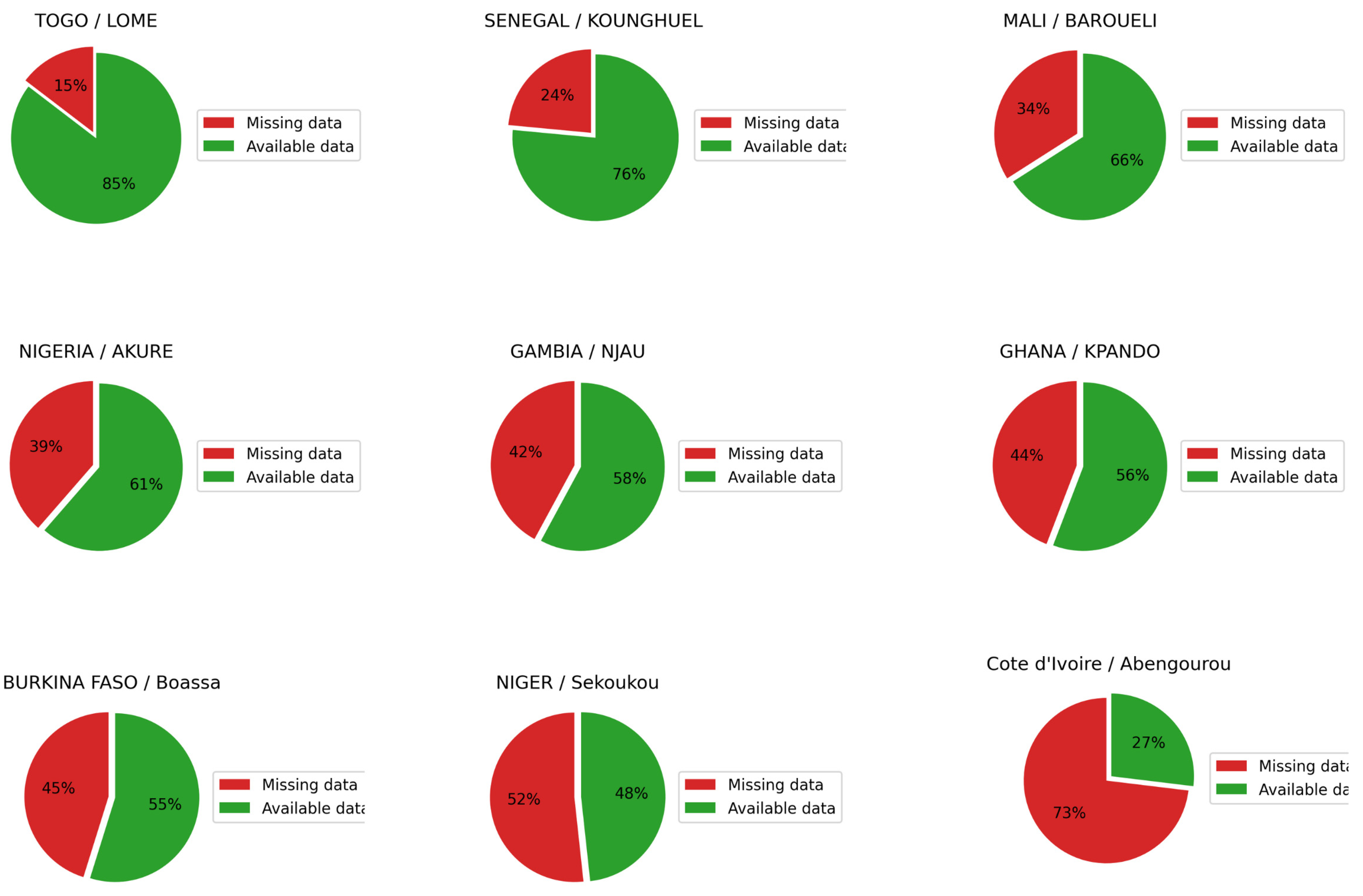
To ensure temporal consistency with auxiliary datasets and reduce high-frequency noise, the quality-controlled 10 min observations were aggregated to an hourly time scale. For each variable, the AWS natively record minimum, maximum, and mean values within each 10 min interval; hourly aggregates were computed by taking the minimum of the six 10 min minima, the maximum of the six 10 min maxima, and the arithmetic mean of the six 10 min mean values, rather than deriving the hourly mean from the hourly minimum and maximum. This procedure preserves the physical meaning of each statistic and avoids the symmetry assumption implicit in approximating the mean as the midpoint between the extrema. Despite the high temporal resolution of the network, data availability varies substantially across stations and variables (Figure 3). Missing data proportions range from less than 10% at the best-covered stations to over 60% at the most affected ones, with strong spatial heterogeneity linked to differences in station maintenance and operational constraints.

2.3. Auxiliary Data Sources

Two external atmospheric datasets were used as auxiliary predictors to support the reconstruction of missing station observations.

Reanalysis data were obtained from ERA5-Land [8], produced by the European Centre for Medium-Range Weather Forecasts (ECMWF) through the Copernicus Climate Change Service (C3S) as a replay of the land-surface component of the ERA5 reanalysis, at a native spatial resolution of approximately 9 km (0.1°) and an hourly temporal resolution. ERA5-Land offers improved representation of land-surface processes compared to the standard ERA5 product, making it particularly suited for near-surface meteorological applications. Relevant fields were extracted at station locations using the nearest grid-point approach, ensuring temporal alignment with the aggregated AWS observations. Despite its strengths, ERA5-Land exhibits systematic biases and scale mismatches relative to station-level observations, particularly for variables governed by local-scale processes such as precipitation and solar radiation [8,9].

For precipitation, satellite-based products from the Global Precipitation Measurement (GPM) mission were used in place of reanalysis-derived rainfall estimates, specifically the Integrated Multi-satellitE Retrievals for GPM (IMERG) Final Run, Version 07 (V07B), at a native spatial resolution of 0.1° (approximately 11 km) and a half-hourly temporal resolution. The Final Run was selected over the near-real-time Early and Late runs because it incorporates a monthly gauge-based climatological adjustment, improving accuracy at the expense of latency (approximately four months after the observation month), which is compatible with the retrospective nature of this study. Half-hourly precipitation estimates were aggregated to hourly totals by summing the two constituent half-hourly values. GPM products provide satellite-based information on precipitation occurrence in tropical convective regimes, which dominate rainfall patterns across West Africa [7]. However, substantial magnitude and detection errors may remain at the station scale because of the spatial mismatch between gridded satellite estimates and point-scale rain-gauge observations. To quantitatively assess the suitability of GPM as an auxiliary precipitation predictor relative to ERA5-Land, a categorical evaluation of rainfall occurrence was performed against available AWS observations. Only timestamps with valid AWS rainfall observations were retained for the evaluation. Rainfall occurrence was represented as a binary event, and product performance was assessed using four categorical verification metrics: Probability of Detection (POD), False Alarm Ratio (FAR), Critical Success Index (CSI), and Heidke Skill Score (HSS). POD measures the fraction of observed rainfall events correctly detected, FAR quantifies the proportion of predicted rainfall events that were not observed, CSI evaluates the correspondence between observed and detected rainfall events while accounting for misses and false alarms, and HSS measures detection skill relative to random agreement. Throughout this study, detailed quantitative results are reported for four representative stations, selected to span distinct agro-climatic zones within the WASCAL network: Lomé (coastal, Togo), Koungheul (Sudanian, Senegal), Akure (humid tropical, Nigeria), and Boassa (Sahelian, Burkina Faso). Station selection was based on this agro-climatic coverage rather than on reconstruction performance, in order to avoid any bias toward the most favorable results.

GPM consistently outperformed ERA5-Land in rainfall-occurrence detection across the four representative stations (

Table 3. Please confirm whether the overlapping/incomplete content in this figure affects scientific understanding and if it does, please revise it.

Station	Product	Number of Valid Observations	Observed Rain Events	Predicted Rain Events	POD	FAR	CSI	HSS
Boassa	ERA5-Land	42,075	243	2284	0.374	0.960	0.037	0.062
	GPM	42,075	243	1307	0.716	0.867	0.126	0.217
Akure	ERA5-Land	46,039	1058	8581	0.511	0.937	0.059	0.074
	GPM	46,039	1058	5418	0.750	0.854	0.140	0.215
Koungheul	ERA5-Land	43,912	452	2807	0.407	0.934	0.060	0.097
	GPM	43,912	452	1579	0.841	0.759	0.230	0.364
Lomé	ERA5-Land	64,684	641	12,299	0.523	0.973	0.027	0.034
	GPM	64,681	641	3819	0.741	0.876	0.119	0.199

). GPM achieved POD values ranging from 0.716 at Boassa to 0.841 at Koungheul, compared with 0.374–0.523 for ERA5-Land. CSI values ranged from 0.119 to 0.230 for GPM, compared with 0.027–0.060 for ERA5-Land, while HSS increased from 0.034 to 0.097 for ERA5-Land to 0.199–0.364 for GPM. The strongest improvement was observed at Koungheul, where GPM achieved POD = 0.841, CSI = 0.230, and HSS = 0.364, compared with 0.407, 0.060, and 0.097, respectively, for ERA5-Land.

Despite this improvement, False Alarm Ratios remained relatively high. FAR values ranged from 0.934 to 0.973 for ERA5-Land and from 0.759 to 0.876 for GPM. Thus, although GPM demonstrated consistently better rainfall-occurrence detection than ERA5-Land, both products remain affected by substantial false detections at the AWS point scale. These results support the use of GPM as the auxiliary precipitation product in the proposed framework while highlighting the limitations associated with representing localized convective rainfall using gridded precipitation products.

ERA5-Land and GPM data were accessed via Google Earth Engine and extracted using a Python-based workflow, ensuring consistent spatial extraction and temporal harmonization across the full study period 2017–2025. The corresponding extraction code is archived and publicly available as described in the Data Availability Statement.

2.4. Data Preprocessing and Quality Control

Reliable reconstruction requires a rigorous preprocessing and quality-control (QC) procedure to ensure that the training dataset is physically consistent and climatologically realistic. A multi-step QC workflow was applied to each station and variable prior to model training.

First, a continuous hourly time axis was generated for each station to explicitly identify missing timestamps and ensure temporal completeness of the dataset structure. Observations were then inspected to remove sensor-inconsistent entries and non-numeric artifacts originating from data transmission or logging issues.

2.4.1. Physical and Climatological Range Checks

Physically implausible values were filtered using variable-specific thresholds based on established climatological knowledge of West Africa [1,2,12]. The following constraints were applied: air temperature was constrained to 5–50 °C, reflecting realistic near-surface conditions across Sahelian, Sudanian, and coastal climates; relative humidity to 0–100%; atmospheric pressure to 960–1090 hPa; global solar radiation values exceeding 1300 W m⁻² were removed; wind speed values above 40 m s⁻¹ were removed, consistent with regional wind climatology [13]; wind direction was constrained to 0–360°; and precipitation values below the instrumental detection limit were set to zero, ensuring consistency with tipping-bucket rain gauge resolution. These filters reduce the influence of spurious measurements while preserving extreme but physically realistic events essential for climate analysis.

2.4.2. Physically Based Pre-Imputation of Global Solar Radiation

Global solar radiation was preprocessed using a physically based constraint enforcing zero radiation during nighttime. For each station and day, local sunrise and sunset times were computed using the Astral Python library [14], which determines solar positions from geographic coordinates, date, and time zone. Radiation values outside the daylight interval were set to zero, ensuring physical consistency of the diurnal radiation cycle and preventing the models from learning unrealistic nighttime radiation patterns.

2.4.3. Assessment of the Missing Data Mechanism

The validity of the proposed gap-filling framework rests on the assumption that statistical relationships learned from available observations remain applicable during missing periods. This assumption depends on the underlying mechanism of missingness. Following the classical taxonomy of Rubin [15], missing data can be classified as Missing Completely at Random (MCAR), where the probability of a value being missing is unrelated to any observed or unobserved variable; Missing at Random (MAR), where this probability depends on other observed variables but not on the missing value itself; or Missing Not at Random (MNAR), where it depends on the unobserved value itself. These mechanisms require different handling strategies, and MNAR cannot be fully verified from observed data alone, since it depends by definition on values that are never observed.

To characterize the missingness mechanism empirically, the distribution of auxiliary meteorological covariates (ERA5-Land temperature, humidity, pressure, wind speed, and solar radiation, and GPM precipitation) was compared between missing and observed periods for each station–variable combination, using the Mann–Whitney U test. This non-parametric test evaluates whether two independent samples originate from the same distribution without assuming normality, making it appropriate for skewed meteorological variables such as precipitation and solar radiation. A statistically significant difference indicates that the probability of missingness is associated with the corresponding covariate, providing evidence against MCAR. Because large sample sizes can yield statistically significant results for differences of negligible practical magnitude, results were additionally screened using the rank-biserial correlation as an effect-size measure, and only differences with both a corrected p-value below 0.05 and a rank-biserial correlation of at least 0.10 were considered meaningful.

As a complementary, circumstantial indicator of a potential MNAR component, conditions in the hours immediately preceding each gap onset were compared to the station’s overall distribution for variables plausibly linked to station power supply (solar radiation, precipitation), using the same testing procedure. This analysis cannot formally confirm an MNAR mechanism, which is inherently unverifiable from observed data, but can reveal circumstantial evidence consistent with it. Results of both analyses are reported in Section 4.4.

2.5. Feature Engineering

After quality control, in situ observations were temporally aligned with auxiliary predictors from ERA5-Land and GPM, resulting in a unified hourly dataset for each station. Feature engineering aimed to identify a reduced set of predictors that are physically meaningful, statistically relevant, and informative for each target variable. Three complementary techniques were used.

First, correlation matrices were computed between candidate predictors and target variables, providing a preliminary assessment of linear relationships and helping identify multicollinearity and physically consistent dependencies. This analysis served as an initial screening tool to remove redundant or weakly informative predictors.

Second, a filter-based feature selection was applied using the SelectKBest method, which ranks predictors according to univariate statistical criteria independently of the learning algorithm. This data-driven approach reduces dimensionality while preserving the most informative features, which is particularly useful for stations with limited valid observations.

Third, SHAP (SHapley Additive exPlanations) values [16] were computed to analyze feature contributions in a more comprehensive manner. Grounded in cooperative game theory, SHAP values quantify the marginal contribution of each predictor to the model output considering all possible feature combinations. Unlike correlation-based measures, SHAP captures nonlinear effects and interactions between variables, allowing both the magnitude and direction of feature influence to be examined.

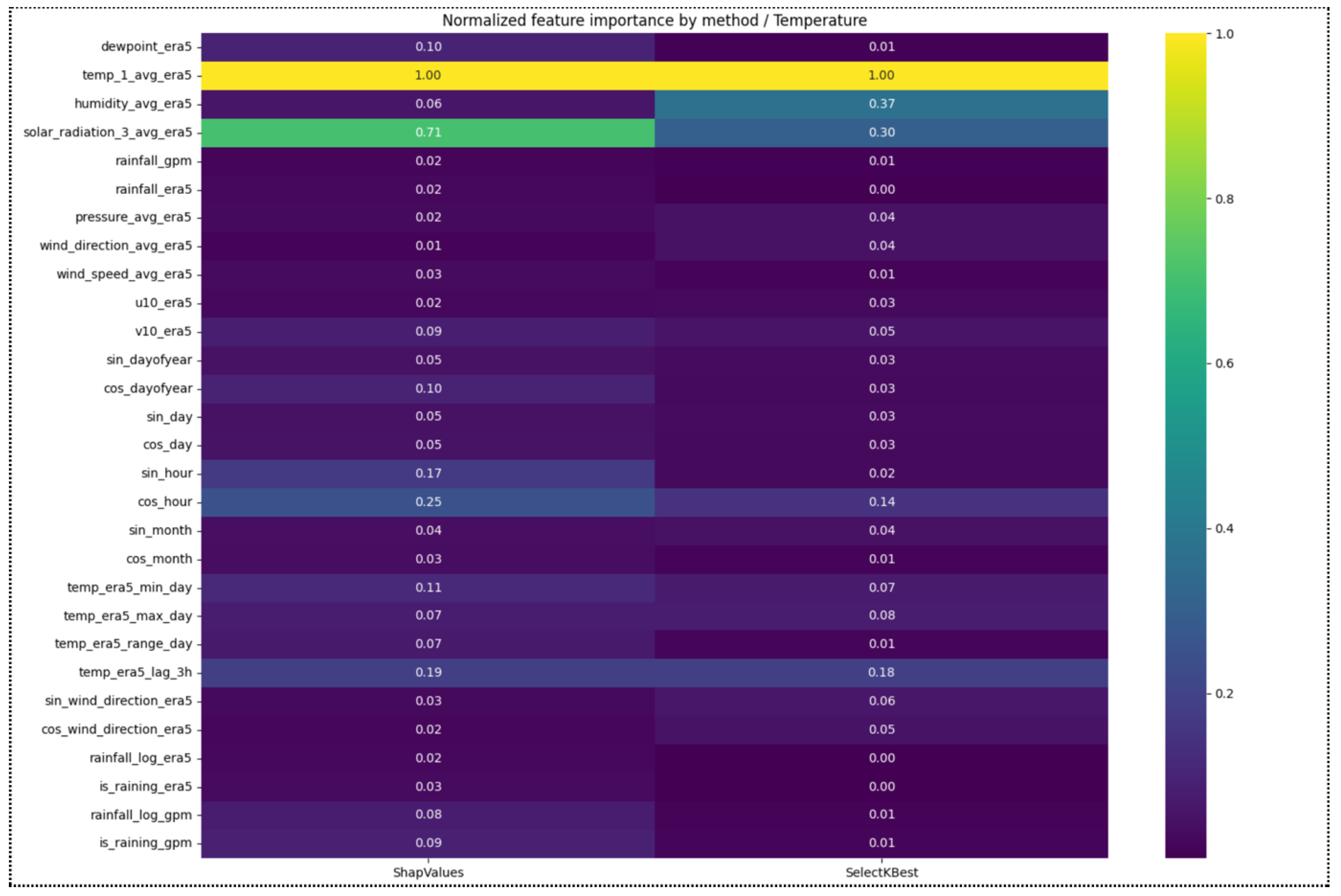
The combined use of these three approaches ensures a robust assessment of predictor relevance, supporting the selection of physically consistent features while maintaining interpretability. The most frequently selected predictors for each target variable, aggregated across all stations, are reported in

Table A1. Most frequently selected predictors per target variable, aggregated across all stations.

Target Variable	Most Frequently Used Features
Temperature	air_temperature_era5, max_temperature_era5, diurnal_temperature_range_era5, dewpoint_temperature_era5, relative_humidity_era5, solar_radiation_avg_era5, cos(hour), sin(day_of_year), cos(wind_direction), rainfall_log
Relative Humidity	relative_humidity_era5, dewpoint_temperature_era5, air_temperature_era5, max_temperature_era5, diurnal_temperature_range_era5, temperature_lag_3h, solar_radiation_avg_era5, sin(day_of_year), cos(day), cos(day_of_year)
Global Solar Radiation	solar_radiation_avg_era5, cos(hour), sin(hour), max_temperature_era5, diurnal_temperature_range_era5, surface_pressure_era5, sin(day_of_year), cos(day), min_temperature_era5, rainfall_indicator
Surface Pressure	surface_pressure_era5, air_temperature_era5, max_temperature_era5, min_temperature_era5, temperature_lag_3h, wind_speed_era5, sin(hour), sin(day_of_year), sin(day), sin(month)
Rainfall	solar_radiation_avg_era5, max_temperature_era5, min_temperature_era5, diurnal_temperature_range_era5, temperature_lag_3h, air_temperature_era5, dewpoint_temperature_era5, sin(day_of_year), cos(day_of_year), sin(wind_direction)
Wind Speed	wind_speed_era5, u10_component_era5, max_temperature_era5, min_temperature_era5, diurnal_temperature_range_era5, dewpoint_temperature_era5, solar_radiation_avg_era5, cos(hour), sin(day_of_year), rainfall_indicator
Wind Direction	wind_direction_era5, sin(wind_direction), cos(wind_direction), u10_component_era5, v10_component_era5, wind_speed_era5, relative_humidity_era5, solar_radiation_avg_era5, diurnal_temperature_range_era5, dewpoint_temperature_era5

(Appendix A). Feature importance results for representative station–variable combinations are illustrated in Figure 4.

In addition to the raw auxiliary fields, several derived variables were constructed to enhance predictor relevance.

2.5.1. Temporal and Cyclical Variables

Meteorological variables exhibit strong temporal structures driven by diurnal and seasonal cycles. Basic calendar descriptors (year, month, day, hour) were included to capture temporal ordering and long-term evolution. To represent periodic behavior without introducing artificial discontinuities, cyclical transformations based on sine and cosine functions were applied to the hour of day, day of month, day of year, and month. These transformations ensure continuity across cycle boundaries (e.g., 23:00–00:00, December–January) and enable the models to learn periodic atmospheric behavior in a physically consistent manner.

2.5.2. Precipitation-Related Variables

Precipitation exhibits a highly skewed distribution with a large proportion of zero values and intermittent extreme events. To better capture these characteristics, GPM-derived precipitation was transformed into three complementary predictors: the raw hourly precipitation amount, a logarithmic transformation to reduce skewness and limit the influence of extreme values, and a binary indicator distinguishing rainy from non-rainy conditions. This decomposition allows the models to separately learn precipitation occurrence and intensity, which is particularly important in tropical regions dominated by convective rainfall.

2.5.3. Temperature and Thermodynamic Variables

Several auxiliary variables were derived from ERA5-Land to represent thermal conditions and short-term persistence effects: daily minimum and maximum air temperature, daily temperature range, hourly mean air temperature, temperature lagged by three hours to capture thermal inertia, and dew point temperature, which provides information on atmospheric moisture content. These variables offer complementary information on diurnal variability, thermal extremes, and short-term temporal dependence.

2.5.4. Atmospheric Pressure and Humidity Variables

Hourly mean surface pressure and relative humidity from ERA5-Land were included as additional predictors. These variables exhibit relatively smooth temporal behavior and are well represented in reanalysis data, making them particularly informative for gap filling.

2.5.5. Wind-Related Variables

Wind observations were characterized using both magnitude and directional information derived from ERA5-Land near-surface wind fields: zonal and meridional components at 10 m height, wind speed computed from these components, and sine-transformed wind direction to preserve angular continuity. The use of vector components and cyclical transformations ensures a physically consistent representation of wind behavior and avoids the discontinuities inherent to angular variables.

2.6. Machine Learning Modeling Strategy

The pattern of missing data in AWS observations is highly heterogeneous, with gaps occurring irregularly and varying in duration. This characteristic strongly constrains the choice of gap-filling methods and excludes approaches that assume regular or weakly missing data structures.

Classical statistical imputation techniques such as Multiple Imputation by Chained Equations (MICE) were initially explored but exhibited poor performance due to the high proportion of missing values and the strong nonlinearity of atmospheric processes [17]. MICE-based reconstructions tended to over-smooth the time series and failed to preserve short-term variability and extremes. Traditional regression models were also found unsuitable, as they require complete input data and rely on linear assumptions rarely satisfied in atmospheric systems. These limitations motivated the adoption of machine learning approaches.

Several algorithms were tested during an exploratory phase on a subset of representative stations, including Random Forest, Extra Trees, Decision Tree, AdaBoost, and LSTM-based models. These models showed either unstable performance across stations or limited ability to reproduce realistic temporal variability and were not retained for large-scale deployment.

The final modeling strategy focused on three gradient boosting-based tree ensemble models: XGBoost, LightGBM, and CatBoost, which demonstrated stable and consistent performance across variables and stations. No fixed minimum sample size was imposed for model training. Because the amount of data required for reliable reconstruction varies substantially across stations and variables, an arbitrary fixed threshold would risk systematically excluding the most data-sparse stations, precisely those for which gap filling is most valuable. A model was therefore trained for every station–variable combination in which the target variable exhibited at least minimal variability, a strict technical requirement given that no relationship can be learned from a constant target.

2.6.1. Multi-Output Regression

For most variables, AWS observations are provided as hourly minimum, mean, and maximum values. Rather than modeling these quantities independently or deriving the mean algebraically from the reconstructed extrema, a multi-output regression strategy was adopted in which the minimum, mean, and maximum are predicted jointly as three separate targets (six targets for wind direction, expressed as sine/cosine pairs for the minimum, mean, and maximum). This approach exploits the intrinsic statistical dependency between the three quantities and avoids the implicit symmetry assumption of an arithmetic average, which does not hold for skewed variables.

The three gradient boosting algorithms differ in how they natively support multi-target regression. For CatBoost, the MultiRMSE loss function was used, which builds a single ensemble of trees shared across all targets, allowing the model to exploit their statistical dependence directly during training. For XGBoost (version ≥ 2.0), the equivalent native strategy is multi_output_tree (with tree_method = ‘hist’), which similarly grows shared trees across targets; this strategy is documented by XGBoost as experimental, with some standard features not yet fully supported, and was validated station by station before full deployment. LightGBM does not currently offer a native multi-output regression strategy; for this algorithm, sklearn.multioutput.MultiOutputRegressor was used instead, training one independent LightGBM model per target with the same hyperparameter configuration. Because the LightGBM targets are trained independently, physical consistency across the three predicted quantities for this algorithm relies entirely on the post-processing constraint described in Section 2.7, whereas for CatBoost and XGBoost this same constraint acts only as a safety net around a relationship already learned jointly during training.

2.6.2. Station-Wise and Variable-Wise Training

For each station–variable combination, feature selection and model training were conducted independently. The set of explanatory variables was not fixed a priori but determined through the feature engineering procedure described in Section 2.5, reflecting local data availability and the physical relevance of candidate predictors. This individualized configuration ensures that each model captures station-specific climatic characteristics rather than relying on a single generalized setup applied uniformly across the network.

2.6.3. Validation Protocol

Model training and evaluation followed a strictly chronological validation design to prevent temporal leakage and ensure that performance estimates reflect realistic operational conditions, applied uniformly across all seven target variables, including precipitation. For each station–variable combination, the complete set of valid co-located observations was first sorted by timestamp. A fixed holdout split was then applied: the first 80% of the chronologically ordered records constituted the training set, and the remaining 20% served as the test set. This partitioning ensures that the model is always evaluated on future observations relative to its training period, consistent with the temporal structure of gap-filling applications. For precipitation, this chronological split preserves the natural imbalance between dry and wet hours within the training and test sets rather than correcting it through random resampling, consistent with the fully chronological design of the pipeline; the resulting class distribution is reported in Section 3.

Hyperparameter optimization was performed using Optuna with a Bayesian search strategy (Tree-structured Parzen Estimator sampler) applied independently for each of the three gradient boosting algorithms, using a fixed random seed (seed = 42) for reproducibility and 30 optimization trials per station–variable–algorithm combination. To prevent the test set from influencing model selection, the training set itself was further split chronologically into an inner training segment (the earliest 85%) and an inner validation segment (the most recent 15%); hyperparameter candidates were scored against this inner validation segment only, and the test set was never accessed during this phase. Random shuffling was excluded from all stages of the pipeline.

For CatBoost, the search space comprised the number of iterations [100, 1000], tree depth [4, 10], learning rate [0.01, 0.3], L2 leaf regularization [1 × 10⁻³, 10] (log scale), bagging temperature [0, 1], and random strength [1 × 10⁻³, 10] (log scale). For XGBoost, the search space comprised the number of estimators [100, 1000], maximum depth [4, 10], learning rate [0.01, 0.3], L2 and L1 regularization [1 × 10⁻³, 10] (log scale), subsample ratio [0.5, 1], column subsample ratio [0.5, 1], and minimum child weight [1, 10]. For LightGBM, the search space comprised the number of estimators [100, 1000], maximum depth [4, 12], number of leaves [15, 255], learning rate [0.01, 0.3], L2 and L1 regularization [1 × 10⁻³, 10] (log scale), subsample ratio [0.5, 1], column subsample ratio [0.5, 1], and minimum child samples [5, 50]; for precipitation only, a Tweedie objective was additionally used, with the Tweedie variance power optimized in [1.01, 1.99]. The selected hyperparameter configuration for each station–variable–algorithm combination is archived in the code repository (see Data Availability Statement). Model training and hyperparameter optimization were performed using CatBoost 1.2.7, XGBoost 2.1.3, LightGBM 4.4.0, and Optuna 4.3.0, with scikit-learn 1.4.2 used for preprocessing and the LightGBM multi-output wrapper, under Python 3.11.5.

2.6.4. Realistic Gap-Masking Evaluation

The chronological holdout described in Section 2.6.3 evaluates the models on a future-extrapolation task, in which the entire test period follows the training period. This differs from the operational gap-filling task, in which missing observations are scattered throughout the record as gaps of variable duration. To assess performance under more realistic conditions, a complementary evaluation was conducted in which artificial gaps were introduced into the complete (non-missing) portion of the training data, with lengths ranging from 1 h to 1 week and probabilities weighted toward shorter, more frequent outages, consistent with the typical duration distribution of AWS network outages. For each station–variable combination, model predictions on these masked segments were compared against the withheld true values, and performance metrics (MAE, RMSE) were stratified by gap length (1–3 h, 4–12 h, 13–24 h, and >24 h) to quantify how reconstruction skill degrades for longer, contiguous outages. This experiment was conducted entirely within the training set, so as not to interfere with the chronological test-set evaluation reported in Section 3.

2.6.5. Baseline Methods

Two baseline gap-filling approaches were implemented to provide reference performance against which the machine learning models were evaluated: linear temporal interpolation and direct substitution using ERA5-Land values.

For the linear interpolation baseline, observed values corresponding to the evaluation period were temporarily masked and reconstructed using linear interpolation along the chronological time series. Interpolation was performed between the nearest available observations surrounding each missing interval. For gaps occurring at the beginning or end of the available series, the nearest available boundary value was used to complete the reconstruction. This baseline represents a simple temporal gap-filling approach relying exclusively on information contained in the AWS time series.

For the ERA5-Land baseline, the masked AWS values were directly replaced by the corresponding ERA5-Land values at the same timestamps. The ERA5-Land variable corresponding most closely to each AWS target variable was used. For variables represented by hourly minimum and maximum AWS observations, the corresponding hourly mean ERA5-Land variable was used as the direct replacement. For precipitation, ERA5-Land precipitation was used directly. For wind direction, the baseline estimates were handled consistently with the machine learning outputs: directional values were represented through sine and cosine components to avoid discontinuities at the 0°/360° boundary, then recombined into physical wind direction angles in the [0°, 360°) range before evaluation. Baseline wind direction performance was therefore assessed using the same circular statistics as the machine learning models, rather than using regression metrics on the sine and cosine components separately.

Baseline performance was evaluated only at timestamps for which both the AWS observation and the corresponding auxiliary value were available. For non-angular variables, the same regression metrics used for the machine learning models were computed between the original AWS observations and the reconstructed baseline values. For wind direction, performance was computed after recombination into degrees using the circular metrics defined in Section 2.6.6.

2.6.6. Model Evaluation and Selection

Model performance was assessed using standard regression metrics computed exclusively on the withheld chronological test set. The mean absolute error (MAE), root mean square error (RMSE), and coefficient of determination (R²) were computed for all variables. The coefficient of determination was calculated as:

$$R^2 = 1 - {\displaystyle \frac{{\displaystyle {\sum }_{i=1}^n}{(y_i - {\hat{y}}_i)}^2}{{\displaystyle {\sum }_{i=1}^n}{(y_i - \overline{y})}^2}}$$

where $y_i$ is the observed value, ${\hat{y}}_i$ is the reconstructed value, $y$ is the mean of the observed values, $n$ and is the number of observations used for evaluation. An $R^2$ value of 1 indicates perfect agreement, whereas $R^2=0$ indicates that the reconstruction performs equivalently to predicting the mean of the observations. Negative $R^2$ values occur when the residual sum of squares exceeds the total sum of squares, indicating that the reconstruction performs worse than using the observed mean as a constant predictor.

For variables with continuous and strictly positive distributions (air temperature, atmospheric pressure, relative humidity, and global solar radiation), the mean absolute percentage error (MAPE) was additionally reported as a normalized error measure. For precipitation, which contains a high proportion of zero values and follows a strongly skewed distribution, the symmetric mean absolute percentage error (sMAPE) was preferred over MAPE as it remains bounded and symmetric when observed values approach zero.

For wind direction, sine and cosine components were predicted jointly as separate targets (Section 2.6.1) but are not reported as standalone metrics, since regression metrics computed directly on these components are not physically meaningful and become statistically unstable as either component approaches zero. Predicted sine and cosine values were instead recombined into a physical wind direction angle in the [0°, 360°) range using the four-quadrant inverse tangent function (Section 2.7), and performance was assessed using circular statistics computed on this recombined angle: the mean angular error, the circular root mean square error, and the proportion of predictions falling within 15°, 30°, and 45° of the observed direction, all of which account for the circular boundary at 0°/360° (e.g., a difference of 2° between 359° and 1°, not 358°).

For each station–variable combination, the best-performing model was selected according to the primary metric appropriate to each variable: R² for continuously distributed non-angular variables, sMAPE for precipitation, and mean angular error for wind direction. The quantitative comparison of model performance across the three algorithms is presented in Section 3.

2.7. Reconstruction and Post-Processing

Once the optimal model was identified for each station–variable combination, the trained models were applied to all periods affected by missing observations to produce continuous hourly time series.

Following prediction, a set of physical plausibility constraints was systematically applied to ensure that all reconstructed values remain within physically meaningful bounds. Precipitation and global solar radiation values were clipped to be non-negative. Relative humidity values were constrained to the interval [0, 100%]. For variables modeled as minimum, mean, and maximum triplets, physical plausibility was enforced as a post-processing safeguard: the reconstructed mean was clipped to lie within the reconstructed minimum and maximum, and the minimum and maximum were reordered where necessary. As detailed in Section 2.6.1, this constraint plays different roles depending on the algorithm: for CatBoost and XGBoost, where the three targets are trained jointly, it acts as a final safety net around an already learned relationship; for LightGBM, where the three targets are trained as independent models, it is the primary mechanism ensuring physical consistency between the reconstructed minimum, mean, and maximum. Wind direction was reconstructed internally through sine and cosine components in order to avoid angular discontinuities during model training. For CatBoost and XGBoost, the sine and cosine targets were learned within a multi-output framework, allowing the model to capture statistical dependencies among the paired directional components and among the minimum, mean, and maximum wind direction targets. Although this strategy does not impose a strict geometric unit-circle constraint on each predicted sine-cosine pair, the final wind direction was not interpreted from the components separately. Instead, each predicted sine-cosine pair was recombined into a physical wind direction angle in the [0°, 360°) range using the four-quadrant inverse tangent function. This conversion uses the orientation of the predicted vector and therefore provides a coherent angular representation before evaluation. Wind direction performance was consequently assessed only after recombination into degrees, using the circular statistics defined in Section 2.6.6.

This procedure produced continuous hourly time series without data gaps, preserving physically consistent temporal variability across all reconstructed variables. The reconstructed datasets constitute the basis for the performance analysis presented in Section 3.

3. Results

This section presents the performance of the machine learning models used to reconstruct missing meteorological observations. Results are analyzed separately for each target variable, with a systematic comparison between XGBoost, LightGBM, and CatBoost. For each variable, model performance is evaluated using the regression metrics defined in Section 2.6.6 and complemented by graphical comparisons between observed and reconstructed time series at four representative stations: Lomé (coastal, Togo), Koungheul (Sudanian, Senegal), Akure (humid tropical, Nigeria), and Boassa (Sahelian, Burkina Faso).

3.1. Air Temperature

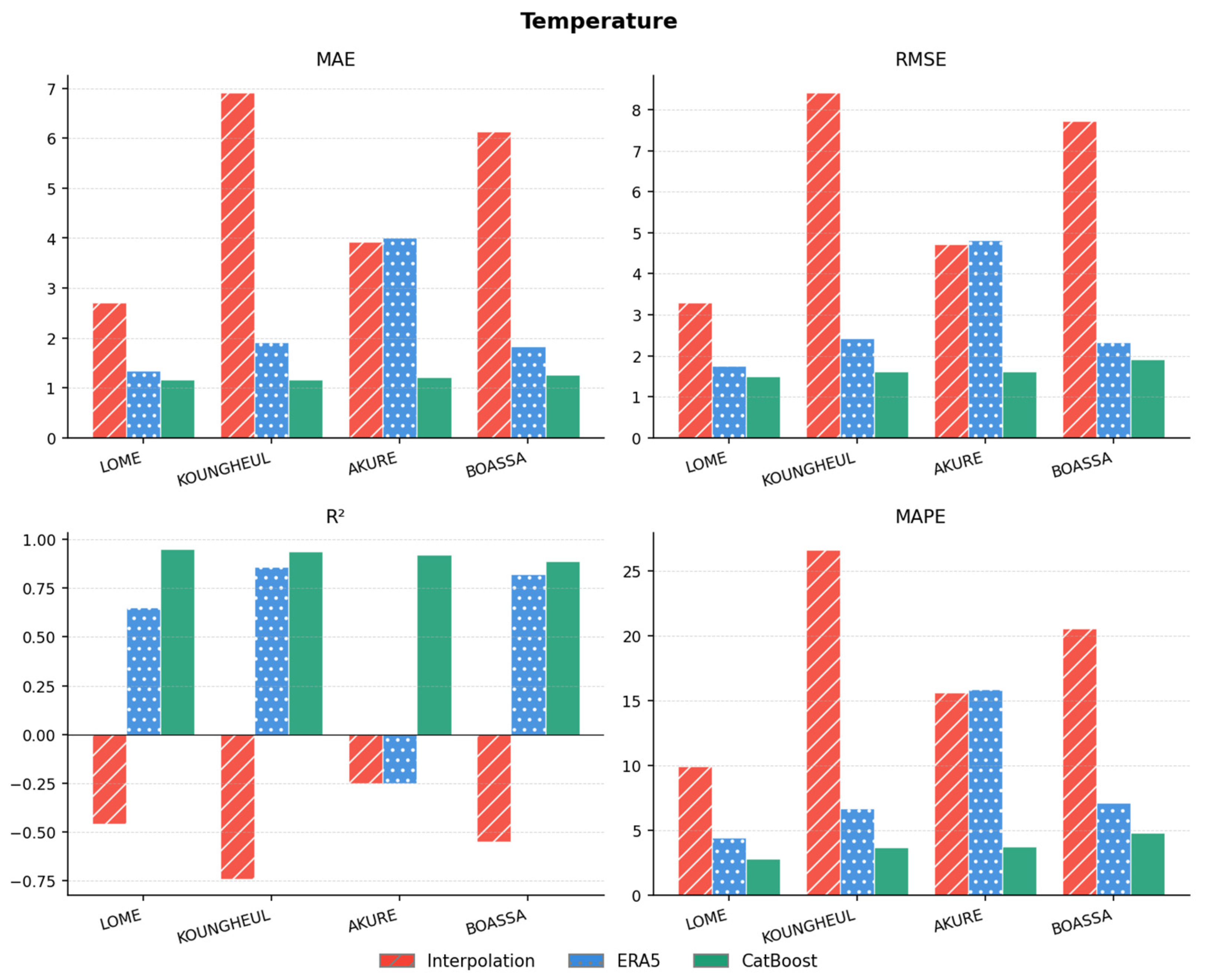
Air temperature reconstruction was performed under the multi-output regression framework, jointly predicting minimum and maximum values. Results are reported here for maximum temperature, which is representative of the overall model behavior. Model performance was compared across the three gradient boosting algorithms and two baseline approaches using MAE, RMSE, R², and MAPE (

Table 4. CatBoost reconstruction performance for maximum hourly air temperature at four representative stations.

Station	MAE (°C)	RMSE (°C)	R2	MAPE (%)
Lomé	1.16	1.50	0.95	2.82
Koungheul	1.17	1.62	0.94	3.67
Akure	1.21	1.61	0.92	3.74
Boassa	1.27	1.92	0.89	4.80

; full comparison in

Table A2. Reconstruction performance metrics (MAE, RMSE, R², MAPE) for maximum hourly air temperature at four representative stations (Lomé, Koungheul, Akure, Boassa), comparing linear interpolation, ERA5-Land direct substitution, XGBoost, LightGBM, and CatBoost.

Station	Method	MAE	RMSE	R2	MAPE (%)
Lomé	Interpolation	2.71	3.30	−0.46	9.94
	ERA5	1.35	1.75	0.65	4.43
	XGBoost	1.30	1.72	0.92	3.35
	LightGBM	1.22	1.62	0.93	3.05
	CatBoost	1.16	1.50	0.95	2.82
Koungheul	Interpolation	6.91	8.41	−0.74	26.61
	ERA5	1.92	2.42	0.86	6.70
	XGBoost	1.33	1.78	0.91	4.30
	LightGBM	1.25	1.70	0.92	3.95
	CatBoost	1.17	1.62	0.94	3.67
Akure	Interpolation	3.92	4.72	−0.25	15.63
	ERA5	4.01	4.82	−0.25	15.88
	XGBoost	1.42	1.99	0.79	5.38
	LightGBM	1.29	1.70	0.90	4.10
	CatBoost	1.21	1.61	0.92	3.74
Boassa	Interpolation	6.13	7.73	−0.55	20.54
	ERA5	1.83	2.32	0.82	7.09
	XGBoost	1.47	2.12	0.85	5.70
	LightGBM	1.36	2.02	0.89	5.20
	CatBoost	1.27	1.92	0.89	4.80

). The visual comparison of CatBoost against both baseline approaches across stations and metrics is provided in Figure 5.

Across all stations, the three models achieve strong performance, with R² values ranging from 0.85 to 0.95 and MAPE below 6%. CatBoost consistently yields the lowest MAE and RMSE and the highest R² at all four stations. The performance advantage is most pronounced at Boassa, where CatBoost achieves an R² of 0.89 compared to 0.85 for XGBoost, likely reflecting the greater sensitivity of this Sahelian station to predictor quality under sparse data conditions.

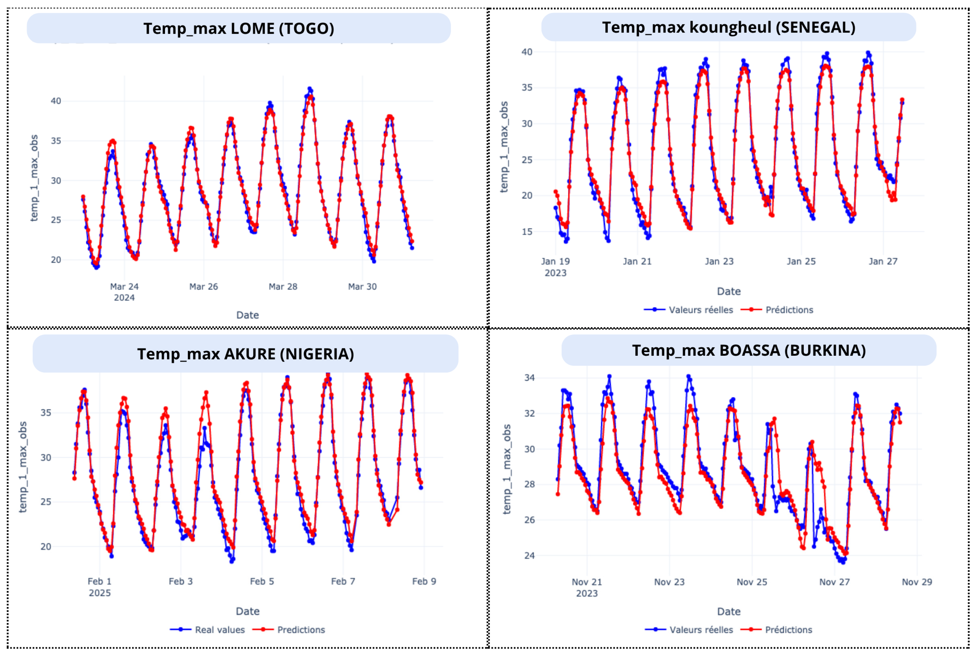
As illustrated in Figure 5, CatBoost substantially outperforms both baseline approaches across all stations and metrics. Linear interpolation yields negative R² values at all four stations (ranging from −0.74 at Koungheul to −0.25 at Akure). As defined in Section 2.6.6, negative R² values indicate that the baseline reconstruction produces larger squared errors than a constant prediction based on the mean of the observed values. These results highlight the limited suitability of linear interpolation for reconstructing gaps of realistic length in a variable with strong diurnal and seasonal variability [5]. ERA5-Land direct substitution performs considerably better at three of the four stations, with R² values of 0.65 at Lomé, 0.86 at Koungheul, and 0.82 at Boassa, consistent with previously reported high correlations between ERA5 and station-level temperature observations [8,9]. At Akure, however, ERA5-Land yields an R² of −0.25, identical to linear interpolation, indicating that reanalysis fields fail to capture the local temperature signal at this humid tropical station. The improvement of CatBoost over ERA5-Land is most notable at Lomé, where R² increases from 0.65 to 0.95, and at Akure, where ERA5-Land’s failure is fully overcome with CatBoost reaching 0.92. These results confirm that the ML framework captures station-scale variability that reanalysis fields alone cannot reproduce at hourly resolution. The observed and reconstructed time series are shown in Figure 6.

3.2. Relative Humidity

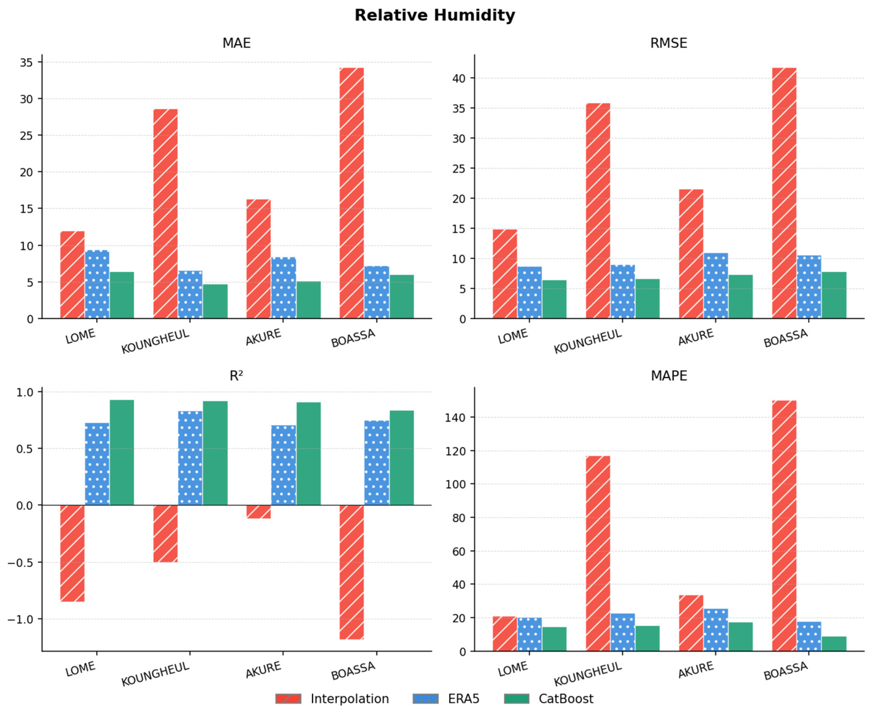
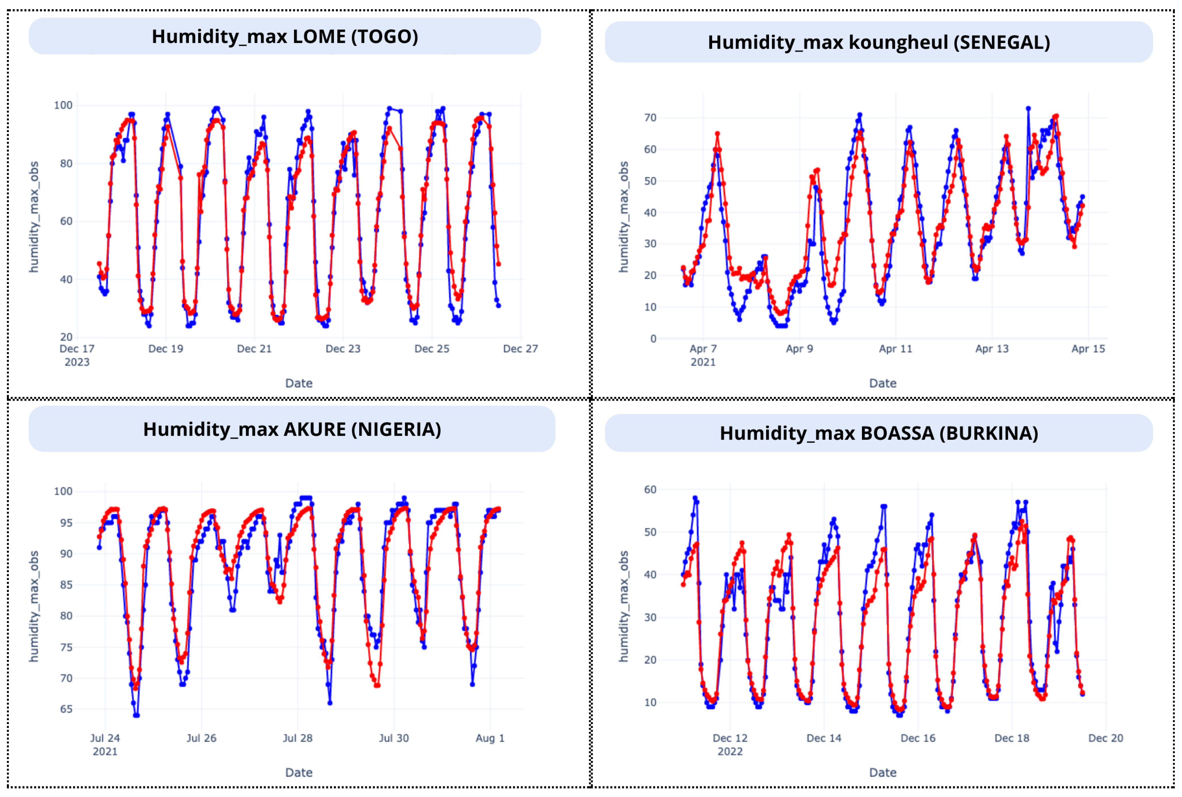
Following the same multi-output regression strategy, relative humidity was reconstructed by jointly predicting minimum and maximum values. Results are reported here for maximum relative humidity, which is representative of the overall model behavior. Model performance was compared across the three gradient boosting algorithms and two baseline approaches using MAE, RMSE, R², and MAPE (

Table 5. CatBoost reconstruction performance for maximum hourly relative humidity at four representative stations.

Station	MAE (% RH)	RMSE (% RH)	R2	MAPE (%)
Lomé	6.46	6.42	0.93	14.66
Koungheul	4.75	6.67	0.92	15.30
Akure	5.16	7.37	0.91	17.46
Boassa	5.98	7.83	0.84	8.96

; full comparison in

Table A3. Reconstruction performance metrics (MAE, RMSE, R², MAPE) for maximum hourly relative humidity at four representative stations (Lomé, Koungheul, Akure, Boassa), comparing linear interpolation, ERA5-Land direct substitution, XGBoost, LightGBM, and CatBoost.

Station	Method	MAE	RMSE	R2	MAPE (%)
Lomé	Interpolation	12.00	14.89	−0.85	21.01
	ERA5	9.4	8.70	0.73	20.50
	XGBoost	8.20	8.40	0.86	19.5
	LightGBM	7.30	7.50	0.89	17.02
	CatBoost	6.46	6.42	0.93	14.66
Koungheul	Interpolation	28.65	35.90	−0.50	116.97
	ERA5	6.60	8.98	0.83	22.88
	XGBoost	6.40	8.60	0.86	21
	LightGBM	5.60	7.60	0.89	18.5
	CatBoost	4.75	6.67	0.92	15.30
Akure	Interpolation	16.30	21.59	−0.12	33.94
	ERA5	8.47	10.99	0.71	25.60
	XGBoost	6.80	9.20	0.85	24
	LightGBM	5.90	8.20	0.87	20.5
	CatBoost	5.16	7.37	0.91	17.46
Boassa	Interpolation	34.24	41.78	−1.18	150.09
	ERA5	7.25	10.57	0.75	18.09
	XGBoost	7.20	9.80	0.78	12.1
	LightGBM	6.60	8.90	0.81	10.5
	CatBoost	5.98	7.83	0.84	8.96

). The visual comparison of CatBoost against both baseline approaches across stations and metrics is provided in Figure 7.

All three models reproduce the observed temporal behavior across stations, capturing diurnal variability and short-term fluctuations with limited systematic bias. CatBoost achieves the best performance at all stations, with R² values ranging from 0.84 at Boassa to 0.93 at Lomé and the lowest MAE across all configurations. Larger deviations between observed and reconstructed values mainly occur during abrupt humidity changes associated with convective events, but overall temporal consistency is preserved.

It is worth noting that MAPE values at Boassa (8.96%) are markedly lower than at other stations (14.66–17.46%), despite a lower R². This reflects the higher mean humidity values at this station, which reduce the relative error metric and highlight the importance of interpreting MAPE alongside absolute metrics such as MAE and RMSE.

As illustrated in Figure 7, CatBoost substantially outperforms both baseline approaches across all stations and metrics. Linear interpolation yields negative R² values at all stations, with the lowest values observed at Boassa (R² = −1.18) and Lomé (R² = −0.85). ERA5-Land direct substitution yields moderate skill, with R² values ranging from 0.71 at Akure to 0.83 at Koungheul, but remains strictly below the ML models at every station on all metrics. The largest gaps between ERA5-Land and CatBoost are observed at Lomé and Akure, where convective humidity fluctuations and local surface conditions are poorly resolved at the reanalysis scale. These results confirm the added value of the ML framework for capturing station-scale humidity dynamics that large-scale reanalysis fields cannot fully represent. The observed and reconstructed time series are shown in Figure 8.

3.3. Global Solar Radiation

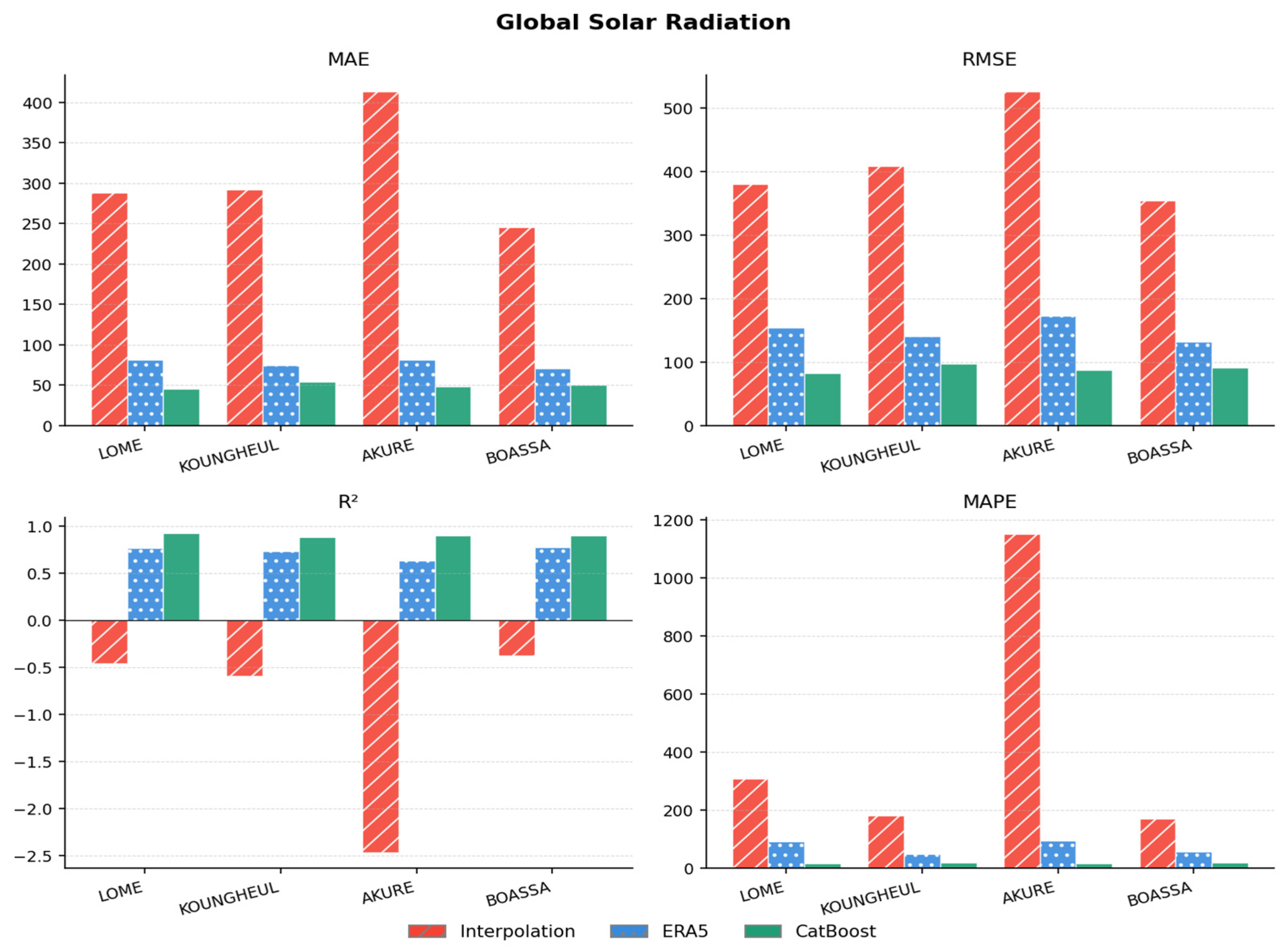
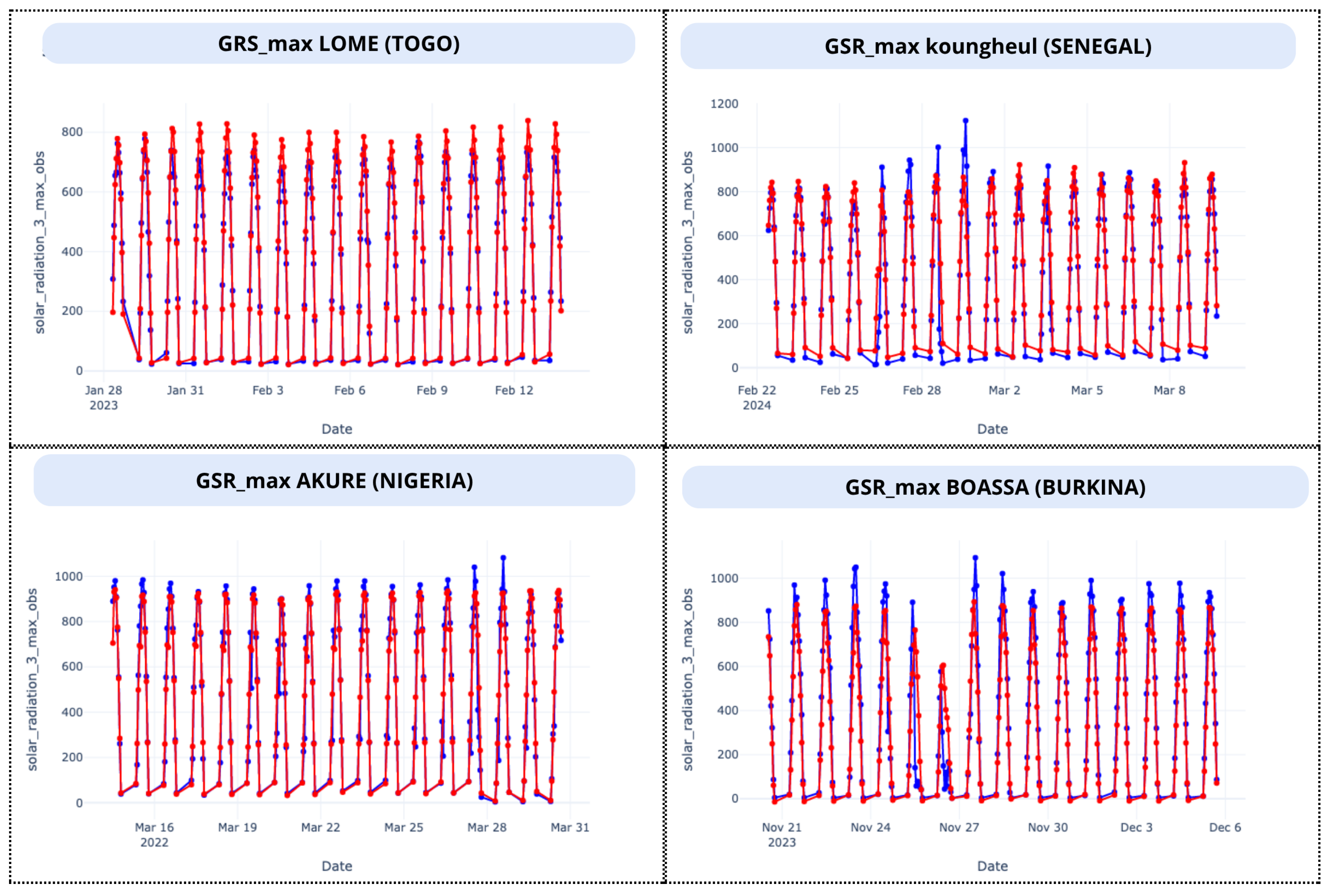
Global solar radiation was reconstructed under the same multi-output regression framework as temperature and humidity, jointly predicting minimum and maximum values. Prior to modeling, nighttime periods were identified using astronomically computed sunrise and sunset times, and radiation values outside the daylight window were set to zero, as described in Section 2.4.3. The multi-output model was therefore applied exclusively to daytime hours, ensuring physical consistency of the diurnal cycle. Model performance was compared across the three gradient boosting algorithms and two baseline approaches using MAE, RMSE, R², and MAPE (

Table 6. CatBoost reconstruction performance for maximum hourly global solar radiation at four representative stations.

Station	MAE (W/m2)	RMSE (W/m2)	R2	MAPE (%)
Lomé	45	82	0.92	15.5
Koungheul	54	98	0.88	18.9
Akure	48	88	0.90	16.8
Boassa	49.95	91.83	0.90	17.32

; full comparison in

Table A4. Reconstruction performance metrics (MAE, RMSE, R², MAPE) for maximum hourly global solar radiation at four representative stations (Lomé, Koungheul, Akure, Boassa), comparing linear interpolation, ERA5-Land direct substitution, XGBoost, LightGBM, and CatBoost.

Station	Method	MAE	RMSE	R2	MAPE (%)
Lomé	Interpolation	287.72	380.16	−0.46	309.03
	ERA5	81.73	154.86	0.76	91.33
	XGBoost	60	110	0.82	22
	LightGBM	52	95	0.87	18.8
	CatBoost	45	82	0.92	15.5
Koungheul	Interpolation	291.55	408.19	−0.59	179.53
	ERA5	75.03	140.76	0.73	47.60
	XGBoost	72	135	0.78	26
	LightGBM	62	115	0.83	22
	CatBoost	54	98	0.88	18.9
Akure	Interpolation	413.18	525.94	−2.46	1151.05
	ERA5	81.57	172.17	0.63	95.43
	XGBoost	66	120	0.80	24
	LightGBM	56	102	0.85	20
	CatBoost	48	88	0.90	16.8
Boassa	Interpolation	245.06	354.85	−0.38	170.47
	ERA5	70.22	132.43	0.77	56.27
	XGBoost	68	125	0.80	24.5
	LightGBM	58	108	0.85	20.5
	CatBoost	49.95	91.83	0.90	17.32

). The visual comparison of CatBoost against both baseline approaches across stations and metrics is provided in Figure 9.

CatBoost outperforms XGBoost and LightGBM at all stations, achieving R² values between 0.88 at Koungheul and 0.92 at Lomé with the lowest MAE in each case. Koungheul exhibits the weakest performance across all models, which may reflect greater cloud variability at this Sudanian station. Larger discrepancies between observed and predicted values mainly occur under highly variable cloudy conditions, where rapid fluctuations in incoming radiation are difficult to capture using hourly reanalysis predictors.

As shown in Figure 9, the performance gap between CatBoost and the baselines is particularly marked for this variable. ERA5-Land direct substitution achieves limited skill across all stations, with R² values ranging from 0.63 at Akure to 0.77 at Boassa, reflecting the inability of reanalysis to represent cloud-driven surface radiation variability at station scale. Linear interpolation performs worse than ERA5-Land at all stations, yielding negative R² values throughout. CatBoost achieves the largest R² gains over ERA5-Land at Akure (+0.27) and Lomé (+0.16), with consistent improvements also recorded at Koungheul (+0.15) and Boassa (+0.13), representing the most substantial relative improvement of the ML framework across all variables. The observed and reconstructed time series are shown in Figure 10.

3.4. Atmospheric Pressure

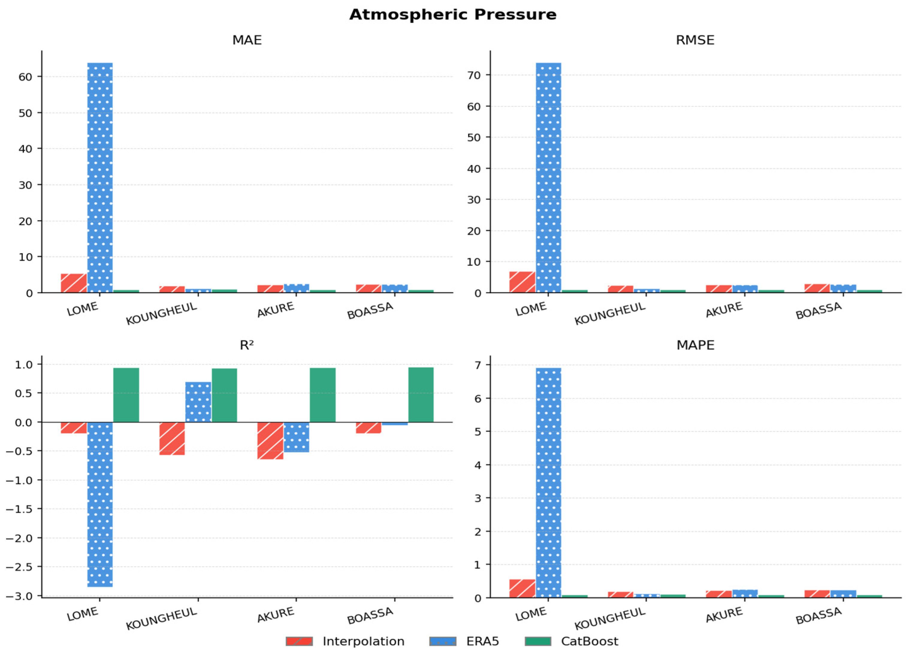
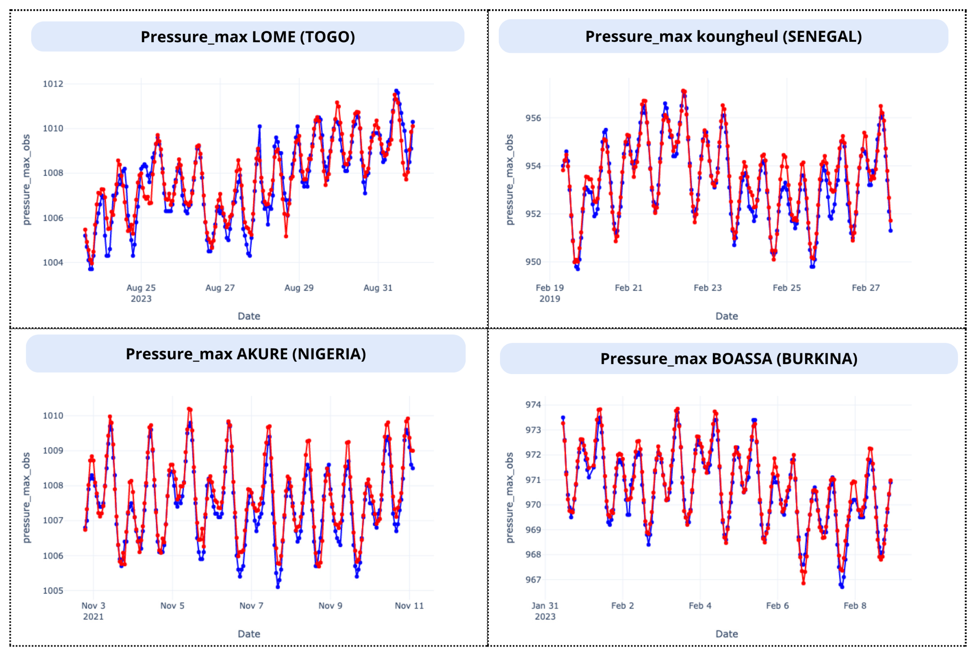
Atmospheric pressure also follows the multi-output regression strategy, with minimum and maximum values predicted jointly. Results are reported here for maximum pressure, which is representative of the overall model behavior. Among all variables, atmospheric pressure yields the highest reconstruction accuracy, with both short-term fluctuations and the semi-diurnal pressure cycle accurately reproduced and minimal deviation between observed and reconstructed values. Model performance was compared across the three gradient boosting algorithms and two baseline approaches using MAE, RMSE, R², and MAPE (

Table 7. CatBoost reconstruction performance for maximum hourly atmospheric pressure at four representative stations.

Station	MAE (hPa)	RMSE (hPa)	R2	MAPE (%)
Lomé	0.92	1.08	0.94	0.10
Koungheul	0.95	1.10	0.93	0.11
Akure	0.93	1.10	0.94	0.10
Boassa	0.89	1.05	0.95	0.09

; full comparison in

Table A5. Reconstruction performance metrics (MAE, RMSE, R², MAPE) for maximum hourly atmospheric pressure at four representative stations (Lomé, Koungheul, Akure, Boassa), comparing linear interpolation, ERA5-Land direct substitution, XGBoost, LightGBM, and CatBoost.

Station	Method	MAE	RMSE	R2	MAPE (%)
Lomé	Interpolation	5.43	6.84	−0.20	0.57
	ERA5	63.87	74.01	−2.85	6.92
	XGBoost	1.10	1.30	0.90	0.14
	LightGBM	1.01	1.18	0.92	0.12
	CatBoost	0.92	1.08	0.94	0.10
Koungheul	Interpolation	1.99	2.47	−0.57	0.20
	ERA5	1.17	1.28	0.70	0.12
	XGBoost	1.15	1.35	0.89	0.15
	LightGBM	1.05	1.22	0.91	0.13
	CatBoost	0.95	1.10	0.93	0.11
Akure	Interpolation	2.16	2.65	−0.65	0.22
	ERA5	2.49	2.56	−0.53	0.26
	XGBoost	1.12	1.32	0.90	0.14
	LightGBM	1.02	1.20	0.92	0.12
	CatBoost	0.93	1.10	0.94	0.10
Boassa	Interpolation	2.31	2.89	−0.20	0.24
	ERA5	2.31	2.71	−0.06	0.24
	XGBoost	0.97	1.15	0.93	0.13
	LightGBM	1.05	1.25	0.91	0.13
	CatBoost	0.89	1.05	0.95	0.09

). The visual comparison of CatBoost against both baseline approaches across stations and metrics is provided in Figure 11.

CatBoost achieves R² values between 0.93 and 0.95 across all stations, with MAE consistently below 1 hPa. The strong performance reflects the large-scale coherence of atmospheric pressure, which is well constrained by ERA5-Land predictors. Boassa shows the best performance across all three ML models, with CatBoost achieving its highest R² (0.95, MAE = 0.89 hPa) and XGBoost also reaching its highest R² at this station (0.93), suggesting that predictor information is particularly well-exploited at this Sahelian location. CatBoost nonetheless consistently reduces both MAE and RMSE relative to XGBoost and LightGBM at all stations, confirming its systematic advantage across the network.

As illustrated in Figure 11, both baseline approaches are clearly outperformed by the ML models at all stations. ERA5-Land direct substitution performs poorly for this variable despite the large-scale nature of pressure fields, with R² values of −2.85 at Lomé, 0.70 at Koungheul, −0.53 at Akure, and −0.06 at Boassa. This unexpectedly weak reanalysis performance likely reflects a systematic elevation or bias correction issue between ERA5-Land grid-point pressure and station-level surface pressure observations, which the ML models effectively learn to correct. Linear interpolation also yields negative R² values at all four stations. CatBoost improves upon ERA5-Land most substantially at Lomé, raising R² from −2.85 to 0.94, and at Akure, where R² rises from −0.53 to 0.94, demonstrating that the ML framework substantially improves the representation of the local pressure signal relative to direct reanalysis substitution. The observed and reconstructed time series are shown in Figure 12.

3.5. Precipitation

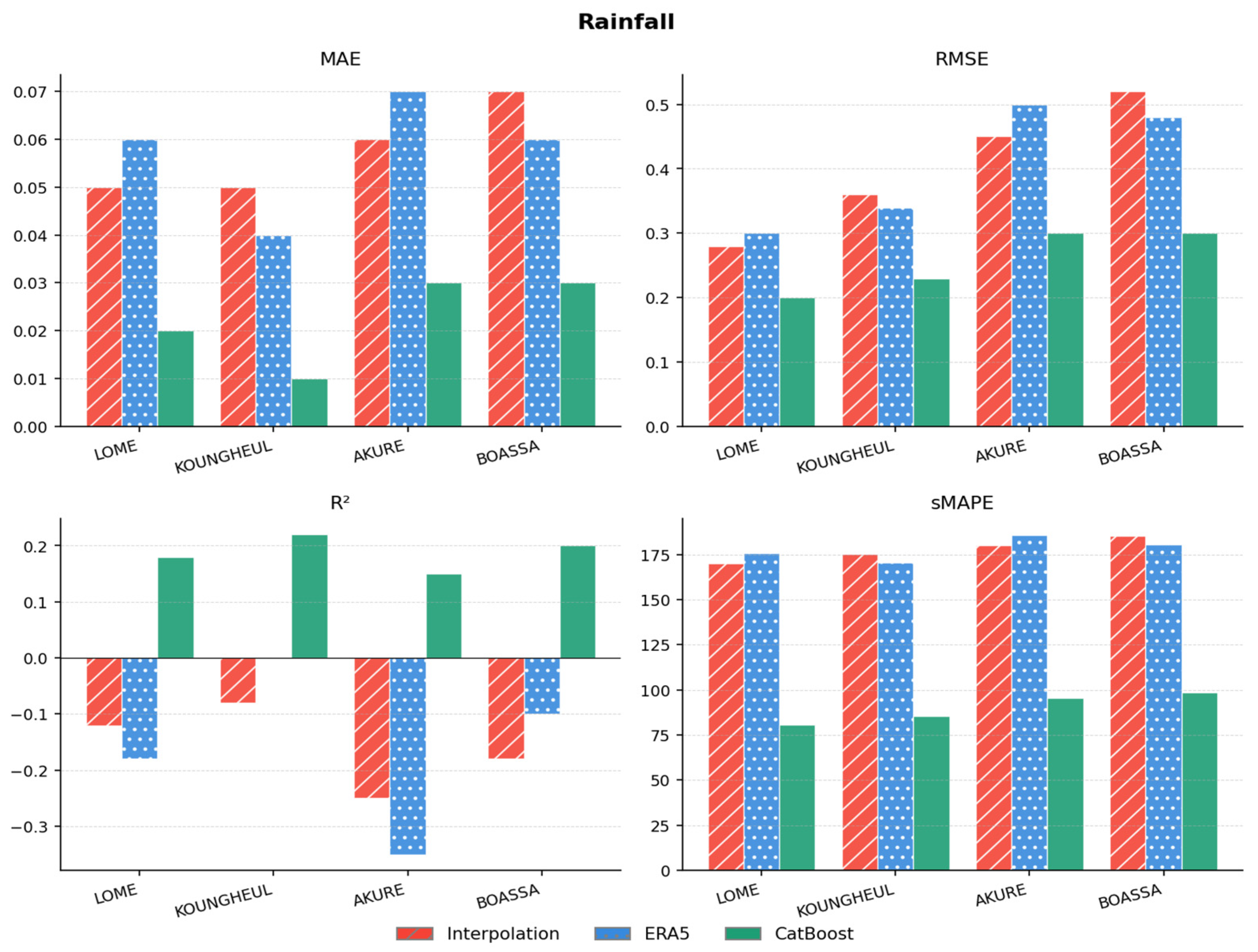
Unlike the other variables, precipitation was modeled as a single target variable and not under a multi-output framework, given the absence of meaningful minimum and maximum distinctions for rainfall accumulation. It was evaluated using sMAPE given the high proportion of zero values and the skewed distribution of rainfall. Model performance was compared across the three gradient boosting algorithms and two baseline approaches (

Table 8. CatBoost reconstruction performance for hourly precipitation at four representative stations.

Station	MAE (mm)	RMSE (mm)	R2	sMAPE (%)
Lomé	0.02	0.20	0.18	80.56
Koungheul	0.01	0.23	0.22	85.49
Akure	0.03	0.30	0.15	95.44
Boassa	0.03	0.30	0.20	98.44

; full comparison in

Table A6. Reconstruction performance metrics (MAE, RMSE, R², sMAPE) for hourly precipitation at four representative stations (Lomé, Koungheul, Akure, Boassa), comparing linear interpolation, ERA5-Land direct substitution, XGBoost, LightGBM, and CatBoost.

Station	Method	MAE	RMSE	R2	sMAPE (%)
Lomé	Interpolation	0.05	0.28	−0.12	170.24
	ERA5	0.06	0.30	−0.18	175.63
	XGBoost	0.04	0.25	0.03	110.47
	LightGBM	0.03	0.22	0.10	95.31
	CatBoost	0.02	0.20	0.18	80.56
Koungheul	Interpolation	0.05	0.36	−0.08	175.14
	ERA5	0.04	0.34	0.00	170.42
	XGBoost	0.03	0.30	0.08	120.38
	LightGBM	0.02	0.26	0.15	100.27
	CatBoost	0.01	0.23	0.22	85.49
Akure	Interpolation	0.06	0.45	−0.25	180.33
	ERA5	0.07	0.50	−0.35	185.71
	XGBoost	0.05	0.40	−0.05	130.18
	LightGBM	0.04	0.34	0.08	110.62
	CatBoost	0.03	0.30	0.15	95.44
Boassa	Interpolation	0.07	0.52	−0.18	185.42
	ERA5	0.06	0.48	−0.10	180.37
	XGBoost	0.05	0.40	0.05	135.21
	LightGBM	0.04	0.34	0.12	115.63
	CatBoost	0.03	0.30	0.20	98.44

). The visual comparison of CatBoost against both baseline approaches across stations and metrics is provided in Figure 13.

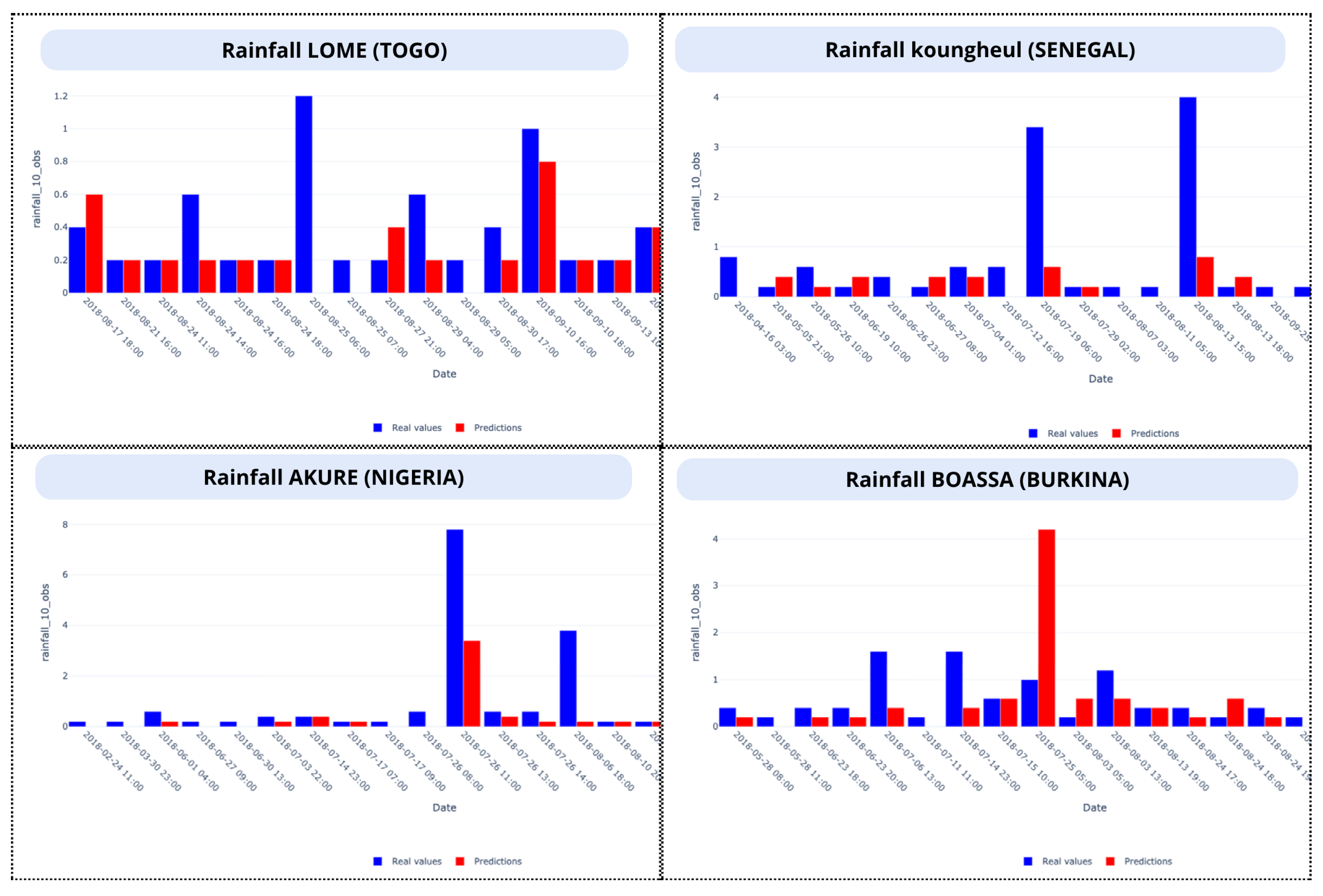
Among the ML models, CatBoost substantially improves upon XGBoost and LightGBM at all stations. At Koungheul, CatBoost achieves the best result across the network with an R² of 0.22 and an sMAPE of 85.49%. At Lomé and Akure, CatBoost yields near-zero or modest R² values (0.18 and 0.15, respectively), confirming the fundamental difficulty of reconstructing convective precipitation from large-scale predictors alone. Overall, the models reproduce part of the distinction between dry and wet periods but systematically underestimate peak rainfall amounts, consistent with the localized and highly intermittent nature of convective precipitation in West Africa.

As shown in Figure 13, both baseline approaches perform substantially worse than the machine learning models for precipitation. ERA5-Land direct substitution yields strongly negative R² values at all four representative stations, indicating performance below the mean-observation reference defined in Section 2.6.6 and highlighting the difficulty of reproducing localized convective rainfall at the AWS point scale [7,8]. Linear interpolation also performs poorly, with sMAPE values of approximately 180–190% across the four stations. The ML framework therefore provides a clear and consistent improvement over both baseline approaches, although absolute reconstruction skill remains limited for precipitation. The observed and reconstructed time series are shown in Figure 14.

3.6. Wind Speed

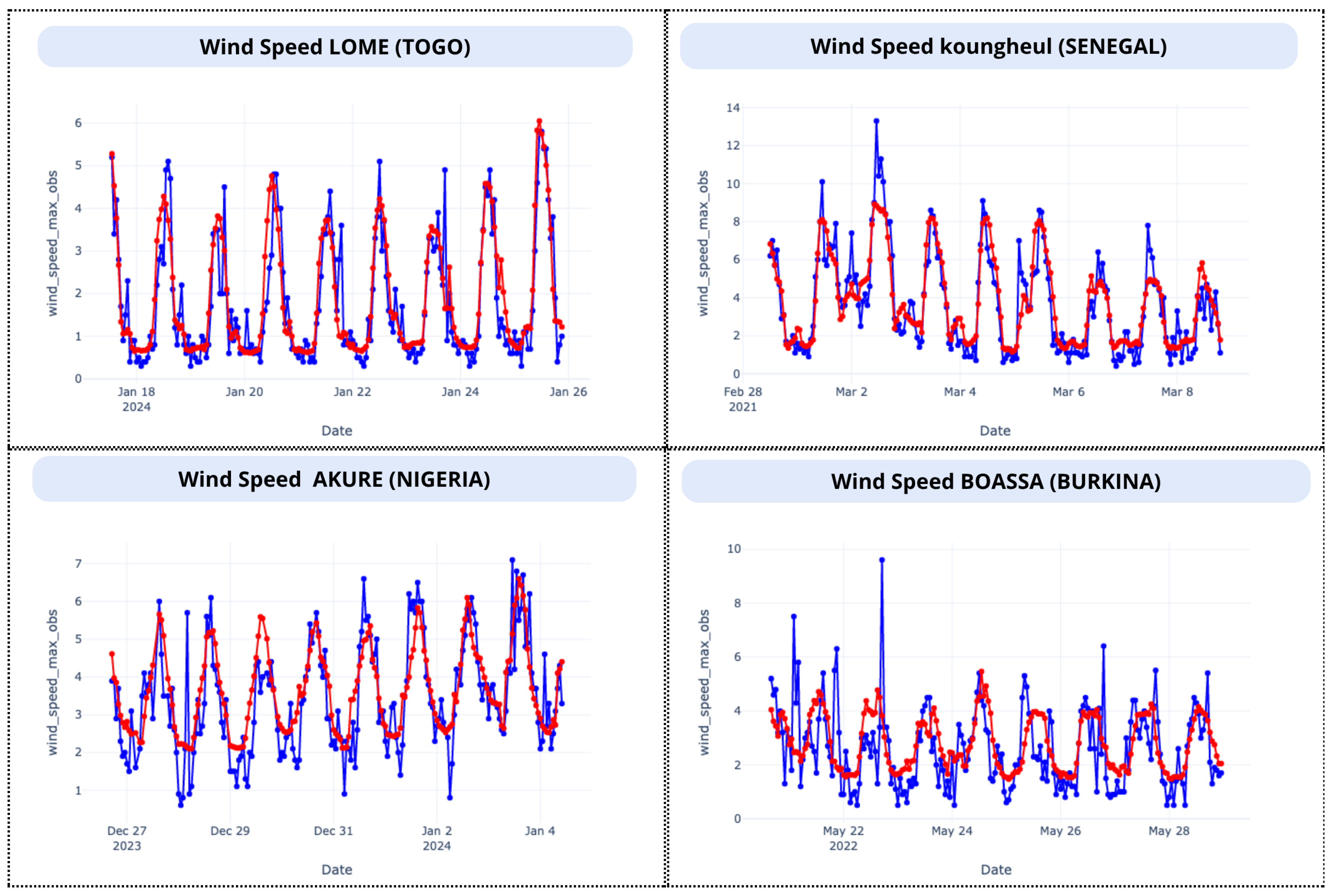
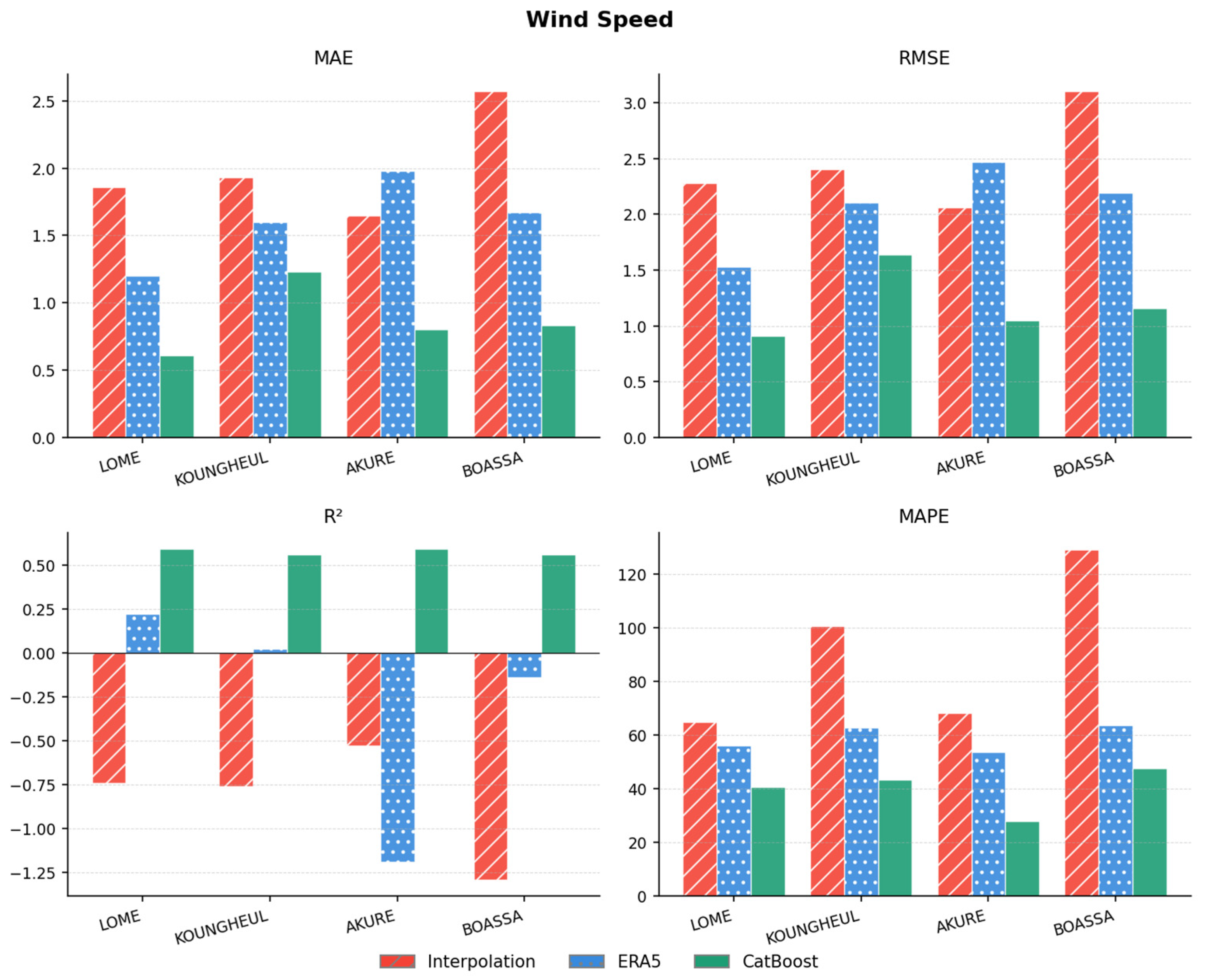
Wind speed reconstruction follows the same multi-output regression strategy as temperature, humidity, radiation, and pressure, with minimum and maximum values predicted jointly. Results are reported here for maximum wind speed, which is representative of the overall model behavior. Reconstructed time series reproduce the main temporal variability and the diurnal cycle with moderate accuracy. Model performance was compared across the three gradient boosting algorithms and two baseline approaches using MAE, RMSE, R², and MAPE (

Table 9. CatBoost reconstruction performance for maximum hourly wind speed at four representative stations.

Station	MAE (m/s)	RMSE (m/s)	R2	MAPE (%)
Lomé	0.61	0.91	0.59	40.43
Koungheul	1.23	1.64	0.56	43.30
Akure	0.80	1.05	0.59	27.86
Boassa	0.83	1.16	0.56	47.51

; full comparison in

Table A7. Reconstruction performance metrics (MAE, RMSE, R², MAPE) for maximum hourly wind speed at four representative stations (Lomé, Koungheul, Akure, Boassa), comparing linear interpolation, ERA5-Land direct substitution, XGBoost, LightGBM, and CatBoost.

Station	Method	MAE	RMSE	R2	MAPE (%)
Lomé	Interpolation	1.86	2.28	−0.74	64.69
	ERA5	1.20	1.53	0.22	56.03
	XGBoost	0.80	1.15	0.45	55.0
	LightGBM	0.70	1.02	0.52	46
	CatBoost	0.61	0.91	0.59	40.43
Koungheul	Interpolation	1.93	2.40	−0.76	100.72
	ERA5	1.60	2.10	0.02	62.71
	XGBoost	1.55	2.05	0.38	58
	LightGBM	1.38	1.82	0.48	50
	CatBoost	1.23	1.64	0.56	43.30
Akure	Interpolation	1.65	2.06	−0.53	68.28
	ERA5	1.98	2.47	−1.19	53.59
	XGBoost	1.05	1.38	0.44	40
	LightGBM	0.92	1.18	0.52	33
	CatBoost	0.80	1.05	0.59	27.86
Boassa	Interpolation	2.57	3.10	−1.29	129.02
	ERA5	1.67	2.19	−0.14	63.50
	XGBoost	0.95	1.33	0.43	52. 37
	LightGBM	1.10	1.50	0.40	62.0
	CatBoost	0.83	1.16	0.56	47.51

). The visual comparison of CatBoost against both baseline approaches across stations and metrics is provided in Figure 15.

CatBoost achieves the best performance at all four stations, with R² values ranging from 0.56 to 0.59 and MAPE between 27.86% and 47.51%. Higher errors are observed during abrupt wind speed changes and extreme gusts, which are systematically underestimated. These deviations reflect the difficulty of representing local wind dynamics using reanalysis-driven predictors, as ERA5-Land does not resolve fine-scale orographic or convective effects that dominate short-lived high-wind events [13].

As illustrated in Figure 15, both baseline approaches are clearly outperformed by the ML models across all stations and metrics. ERA5-Land direct substitution yields negative or near-zero R² values at three of the four stations (−1.19 at Akure, −0.14 at Boassa, and 0.02 at Koungheul). At Lomé, ERA5-Land achieves a positive but modest R² of 0.22, remaining substantially below all ML models on every metric. Linear interpolation yields negative R² values at all stations. The ML framework provides a substantial improvement over both baselines, with CatBoost raising R² from negative or near-zero values to 0.56 to 0.59 across all stations. The moderate absolute performance nonetheless highlights the fundamental challenge of reconstructing a variable strongly governed by local-scale processes not captured by the available predictors. The observed and reconstructed time series are shown in Figure 16.

3.7. Wind Direction

Wind direction was evaluated after recombination into physical angles in degrees, following the circular-statistics procedure defined in Section 2.6.6 and Section 2.7. Results are reported here for the hourly average wind direction, using mean angular error, circular RMSE, and the proportions of predictions falling within 15° and 30° of the observed direction. The full comparison across methods is provided in

Table A8. Circular reconstruction performance metrics for hourly average wind direction after recombination into physical angles in degrees, comparing CatBoost, XGBoost, LightGBM, ERA5-Land direct substitution, and linear interpolation.

Station	Method	Mean Angular Error (°)	Circular RMSE (°)	Within 15° (%)	Within 30° (%)	Within 45° (%)
Boassa	CatBoost	35.4	50.8	35.9	59.7	—
Boassa	XGBoost	35.6	51.0	35.4	59.6	73.6
Boassa	LightGBM	—	—	—	—	—
Boassa	ERA5-Land	38.3	55.1	34.3	57.1	71.0
Boassa	Linear interpolation	120.8	130.4	5.7	9.8	12.4
Akure	CatBoost	37.4	52.9	33.1	57.0	—
Akure	XGBoost	37.4	53.2	33.4	57.0	72.0
Akure	LightGBM	37.4	53.2	33.1	57.2	72.0
Akure	ERA5-Land	39.3	55.0	30.2	54.2	70.0
Akure	Linear interpolation	60.2	72.9	15.1	28.6	40.3
Koungheul	CatBoost	34.3	51.1	40.6	62.8	—
Koungheul	XGBoost	34.0	51.2	41.3	63.4	75.6
Koungheul	LightGBM	34.6	51.5	39.9	62.6	74.8
Koungheul	ERA5-Land	48.2	67.1	27.7	49.0	63.3
Koungheul	Linear interpolation	97.8	112.1	6.3	14.5	23.8
Lomé	CatBoost	20.4	34.2	60.3	81.6	—
Lomé	XGBoost	20.5	34.3	60.1	81.5	89.2
Lomé	LightGBM	20.4	34.3	60.2	81.5	89.3
Lomé	ERA5-Land	24.0	37.8	51.1	76.7	86.1
Lomé	Linear interpolation	33.4	45.8	36.5	59.7	73.1

.

Table 10. CatBoost reconstruction performance for hourly average wind direction after recombination into physical angles in degrees at four representative stations.

Station	Mean Angular Error (°)	Circular RMSE (°)	Within 15° (%)	Within 30° (%)
Lomé	20.4	34.2	60.3	81.5
Koungheul	34.3	51.1	40.6	62.8
Akure	37.4	52.9	33.1	57
Boassa	35.4	50.8	35.9	59.7

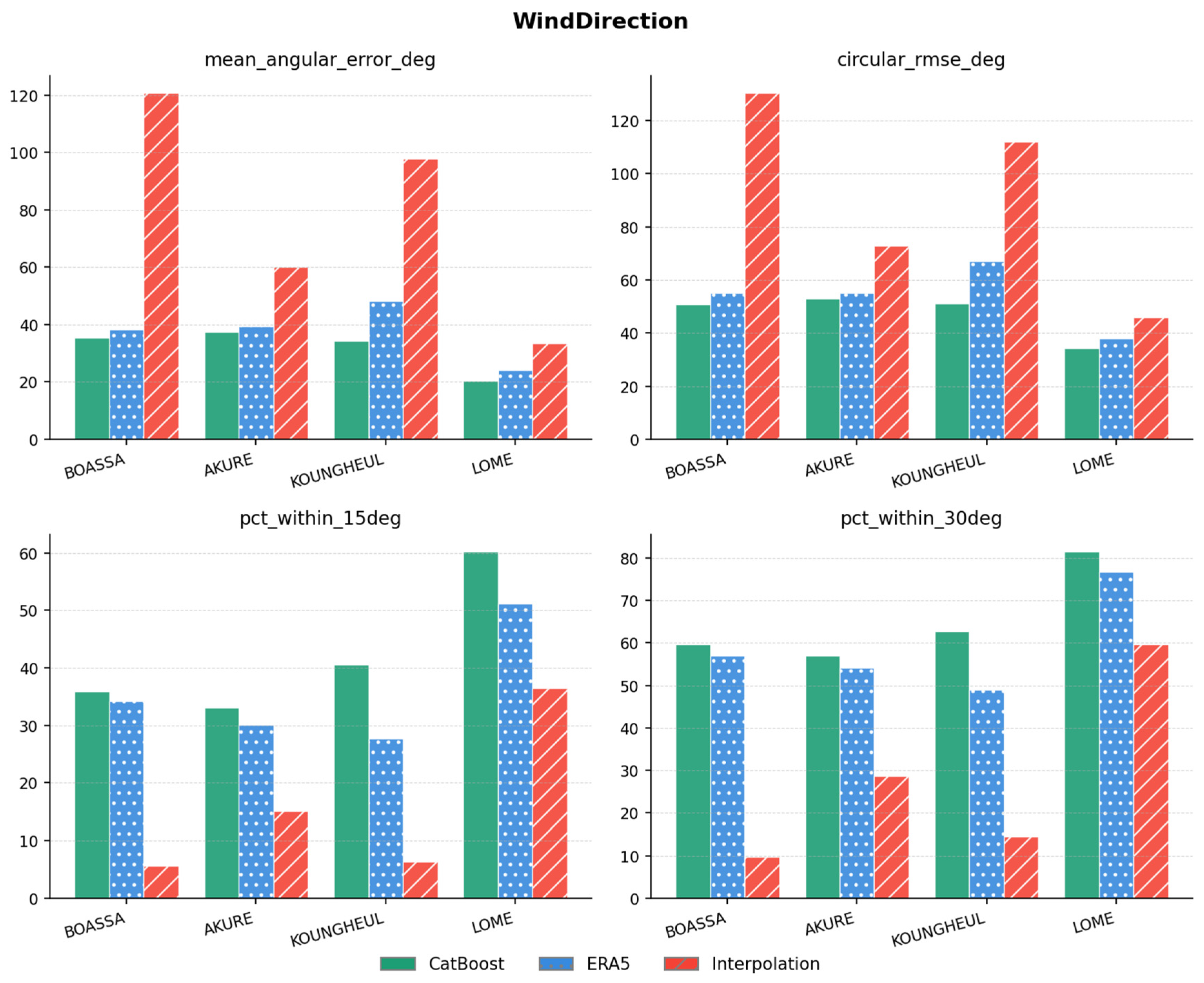
summarizes the CatBoost performance for the four representative stations. Across stations, wind direction remained the most challenging variable to reconstruct. CatBoost achieved mean angular errors ranging from 20.4° at Lomé to 37.4° at Akure, with circular RMSE values ranging from 34.2° to 52.9°. The best performance was obtained at Lomé, where 60.3% of predictions fell within 15° of the observed direction and 81.6% fell within 30°. At Boassa and Akure, only about one-third of predictions were within 15°, although the proportion within 30° remained close to 57–60%. Koungheul showed an intermediate pattern, with a mean angular error of 34.3° and 62.8% of predictions within 30°.

Figure 17 compares the circular-statistics-based performance of CatBoost with ERA5-Land direct substitution and linear interpolation. CatBoost consistently produced lower mean angular error and circular RMSE than both baseline approaches. The improvement was particularly strong against linear interpolation, especially at Boassa and Koungheul, where interpolation yielded mean angular errors of 120.8° and 97.8°, respectively. ERA5-Land direct substitution performed better than interpolation at most stations but remained less accurate than CatBoost across all four stations. The advantage of CatBoost was also reflected in the tolerance-based metrics, with higher proportions of predictions falling within both 15° and 30° of the observed direction.

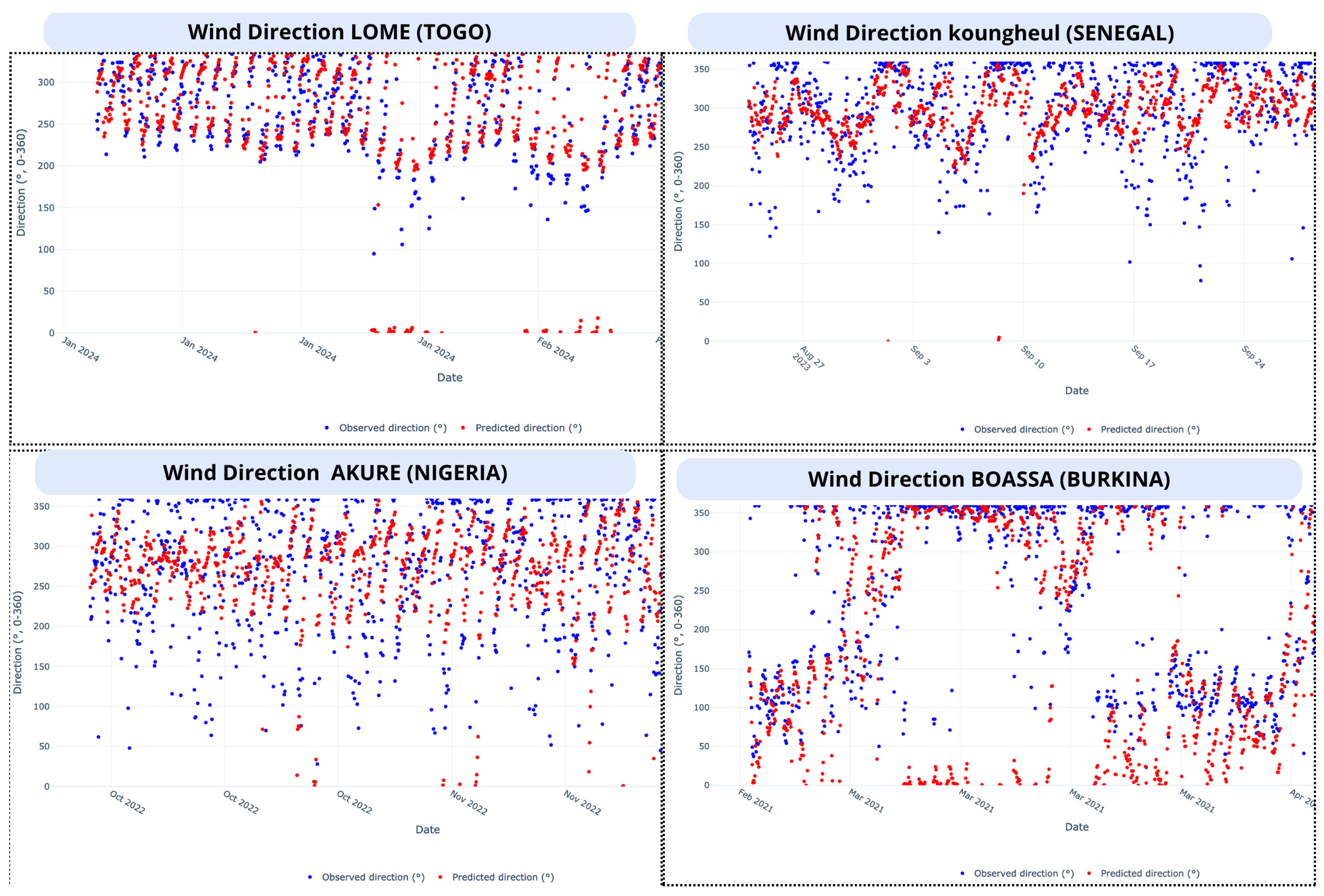
The observed and reconstructed wind direction angles are shown in Figure 18. Points are displayed without connecting lines to avoid artificial visual continuity across the 0°/360° boundary. This representation is more appropriate for angular variables, since two consecutive values close to 360° and 0° are physically close even though they appear numerically far apart on a linear axis.

The comparatively weak performance of wind direction is consistent with its strong dependence on local-scale processes. Directional changes are influenced by station exposure, nearby obstacles, surface roughness, local topography, and convective outflows, which are not fully represented by the available large-scale predictors. The model therefore captures part of the dominant directional regime but remains limited in reproducing abrupt hourly shifts.

3.8. Summary of Reconstruction Performance

Taken together, the results across all seven reconstructed variables reveal a clear hierarchy in reconstruction skill closely linked to the physical nature of each variable. CatBoost systematically outperforms XGBoost and LightGBM at all stations, with the performance gap widening for the more challenging variables.

Atmospheric pressure and air temperature exhibit the highest reconstruction skill, with R² values typically exceeding 0.90 and MAPE below 5%. Relative humidity and global solar radiation are reliably reconstructed with R² values between 0.84 and 0.93, though with higher sensitivity to station-specific conditions such as cloud variability and convective events.

Precipitation represents the most challenging scalar variable, with R² values ranging from 0.15 to 0.22 and sMAPE values between 80% and 98%, reflecting the difficulty of capturing convective rainfall dynamics from large-scale predictors. Wind speed achieves moderate performance with R² between 0.56 and 0.59. Wind direction yields the weakest overall performance when assessed with circular statistics after angular recombination, with mean angular errors ranging from 20.4° to 37.4° and circular RMSE values from 34.2° to 52.9°.

4. Discussion

This section discusses the main findings of this study in relation to the physical characteristics of the target variables, the role of data availability and auxiliary predictors, and the limitations of the proposed framework.

4.1. Variable-Specific Reconstruction Performance

The results reveal a clear hierarchy in reconstruction skill closely linked to the physical nature of each variable. Air temperature and atmospheric pressure achieve the highest accuracy, attributable to their strong temporal persistence, large-scale spatial coherence, and close relationship with ERA5-Land fields. These properties make them particularly amenable to supervised learning, as reanalysis predictors provide highly informative representations of the underlying physical processes. These findings are consistent with previous studies reporting high correlations between ERA5 and station-level temperature and pressure observations [8,9]. Relative humidity and global solar radiation exhibit robust but slightly lower performance. For humidity, the main source of error lies in abrupt fluctuations associated with convective events, which are poorly resolved at the reanalysis scale. For solar radiation, performance is sensitive to cloud variability, particularly at Sudanian stations such as Koungheul where convective cloud cover exhibits high intermittency. The physically based pre-imputation of nighttime radiation described in Section 2.4.3 contributes positively by eliminating a source of spurious variance and allowing the models to focus on daytime dynamics.

Precipitation and wind-related variables remain the most challenging. Rainfall reconstruction correctly captures occurrence patterns but systematically underestimates extreme intensities. This behavior reflects the localized and intermittent nature of convective precipitation in West Africa, where rainfall events are driven by mesoscale convective systems not resolved by ERA5-Land or GPM at the station scale [6,7,8]. The negative R² values at Lomé and Akure indicate that, at certain stations, the available predictor set is insufficient to capture the rainfall signal. Wind speed and direction exhibit similar limitations, as local-scale orographic and convective effects that dominate short-lived wind events are not represented in reanalysis fields [13].

4.2. Influence of Data Availability on Model Performance

Model performance clearly degrades as the proportion of missing data increases at the variable level. Variables with sufficient observational coverage yield stable and accurate reconstructions, whereas variables affected by extensive and persistent gaps show reduced skill. This effect is particularly pronounced for precipitation and wind, which already present intrinsic modeling difficulties.

After quality control, some variables at specific stations did not retain enough valid observations to support supervised learning. In such cases, no model was trained for the affected variable, while other variables at the same station were successfully reconstructed. This confirms that data availability constraints operate at the variable level rather than the station level, consistent with established findings on the minimum data requirements for supervised learning in climate applications [18,19]. This distinction is important: the absence of a trained model for a given variable should be interpreted as a data limitation rather than a failure of the overall framework.

4.3. Role of Multi-Source Predictors and Feature Selection

The integration of multi-source auxiliary data plays a central role in the overall performance of the framework. ERA5-Land variables provide physically consistent large-scale information that is particularly effective for thermodynamic variables, while GPM-derived products provide more informative satellite-based estimates of rainfall occurrence. The categorical comparison between GPM and ERA5-Land confirms this distinction, with GPM consistently achieving higher POD, CSI, and HSS and lower FAR across the four representative stations. However, the relatively high FAR values obtained with GPM indicate that satellite precipitation estimates still have substantial difficulty in reproducing localized convective rainfall at individual AWS locations. Derived predictors, including temporal encodings and lagged variables, further enhance the models’ ability to capture persistence and cyclical behavior.

Feature selection analyses based on SelectKBest and SHAP values described in Section 2.5 and illustrated in Figure 4 confirm that the most influential predictors are physically consistent with the target variables: thermodynamic fields dominate temperature and humidity models, radiation-related variables and temporal features are essential for solar radiation, and satellite-derived indicators are central for precipitation. This agreement between model-driven interpretation and established atmospheric knowledge supports the physical credibility of the reconstructed time series.

Regarding model selection, CatBoost consistently outperforms XGBoost and LightGBM across all variables, with the performance gap widening for the more challenging variables. This advantage may be attributed to CatBoost’s ordered boosting and symmetric tree structure, which reduce overfitting and improve generalization, particularly in settings with heterogeneous feature types and moderate training set sizes [10]. This finding aligns with recent comparative studies suggesting that CatBoost offers competitive or superior performance for environmental regression tasks.

4.4. Limitations

Several limitations should be acknowledged. First, the framework relies on the assumption that relationships learned from available observations remain valid during gap periods. If missing data systematically coincided with specific meteorological conditions, reconstructed values could be biased toward more common atmospheric states. In this network, however, data gaps arise mainly from sensor failures, battery depletion, vandalism, and connectivity problems, all of which are rooted in maintenance capacity and infrastructure rather than meteorological conditions. To assess this assumption empirically rather than qualitatively, the missingness mechanism was tested against auxiliary meteorological covariates following the procedure described in Section 2.4.3. The MCAR hypothesis was rejected with a non-negligible effect in 75% of the station–variable combinations tested (

Table A9. Missingness mechanism assessment by station and variable for the four representative stations, showing the MCAR test result and driving covariate (left) and the circumstantial MNAR indicator and driving precursor (right), as described in Section 2.4.3.

Station	Variable	% Miss	MCAR (H0)	Driving Covariate (MCAR)	r	p	MNAR	Driving Precursor (MNAR)	r	p
Akure	Temperature	38.9	Not rejected	Wind speed (ERA5)	−0.07	<0.001	Present	Rainfall (GPM)	−0.27	<0.001
Akure	Humidity	57.6	Rejected	Humidity (ERA5)	−0.36	<0.001	Present	Rainfall (GPM)	−0.28	<0.001
Akure	Pressure	38.9	Not rejected	Wind speed (ERA5)	−0.07	<0.001	Present	Rainfall (GPM)	−0.27	<0.001
Akure	Rainfall	35.0	Not rejected	Solar rad. (ERA5)	0.08	<0.001	Present	Solar rad. (ERA5)	−0.41	<0.001
Akure	SolarRadiation	16.2	Rejected	Solar rad. (ERA5)	−0.58	<0.001	Present	Rainfall (GPM)	−0.14	<0.001
Akure	WindSpeed	35.7	Not rejected	Solar rad. (ERA5)	0.08	<0.001	Present	Solar rad. (ERA5)	−0.41	<0.001
Akure	WindDirection	35.7	Not rejected	Solar rad. (ERA5)	0.08	<0.001	Present	Solar rad. (ERA5)	−0.41	<0.001
Koungheul	Temperature	22.0	Rejected	Humidity (ERA5)	0.10	<0.001	Absent	Solar rad. (ERA5)	−0.22	0.663
Koungheul	Humidity	22.0	Rejected	Humidity (ERA5)	0.10	<0.001	Absent	Solar rad. (ERA5)	−0.22	0.663
Koungheul	Pressure	22.0	Rejected	Humidity (ERA5)	0.10	<0.001	Absent	Solar rad. (ERA5)	−0.22	0.663
Koungheul	Rainfall	22.0	Rejected	Humidity (ERA5)	0.10	<0.001	Absent	Solar rad. (ERA5)	−0.22	0.663
Koungheul	SolarRadiation	11.5	Rejected	Solar rad. (ERA5)	−0.56	<0.001	Present	Solar rad. (ERA5)	0.34	<0.001
Koungheul	WindSpeed	22.0	Rejected	Humidity (ERA5)	0.10	<0.001	Present	Solar rad. (ERA5)	−0.13	0.717
Koungheul	WindDirection	22.0	Rejected	Humidity (ERA5)	0.10	<0.001	Absent	Solar rad. (ERA5)	−0.22	0.663
Lomé	Temperature	8.7	Rejected	Temp. (ERA5)	0.30	<0.001	Absent	Solar rad. (ERA5)	−0.13	0.531
Lomé	Humidity	8.9	Rejected	Temp. (ERA5)	0.30	<0.001	Present	Rainfall (GPM)	−0.44	<0.001
Lomé	Pressure	46.5	Rejected	Humidity (ERA5)	−0.37	<0.001	Present	Solar rad. (ERA5)	−0.20	<0.001
Lomé	Rainfall	8.7	Rejected	Temp. (ERA5)	0.30	<0.001	Absent	Solar rad. (ERA5)	−0.13	0.531
Lomé	SolarRadiation	4.8	Rejected	Solar rad. (ERA5)	−0.48	<0.001	Present	Solar rad. (ERA5)	0.18	<0.001
Lomé	WindSpeed	9.7	Rejected	Pressure (ERA5)	−0.25	<0.001	Present	Solar rad. (ERA5)	−0.17	<0.001
Lomé	WindDirection	8.7	Rejected	Temp. (ERA5)	0.30	<0.001	Absent	Solar rad. (ERA5)	−0.13	0.531
Boassa	Temperature	38.7	Rejected	Humidity (ERA5)	−0.24	<0.001	Present	Solar rad. (ERA5)	−0.14	<0.001
Boassa	Humidity	41.9	Rejected	Humidity (ERA5)	−0.31	<0.001	Present	Rainfall (GPM)	−0.17	<0.001
Boassa	Pressure	38.7	Rejected	Humidity (ERA5)	−0.24	<0.001	Present	Solar rad. (ERA5)	−0.14	<0.001
Boassa	Rainfall	38.7	Rejected	Humidity (ERA5)	−0.24	<0.001	Present	Solar rad. (ERA5)	−0.14	<0.001
Boassa	SolarRadiation	20.4	Rejected	Solar rad. (ERA5)	−0.58	<0.001	Present	Solar rad. (ERA5)	0.34	<0.001
Boassa	WindSpeed	55.3	Not rejected	Humidity (ERA5)	−0.07	<0.001	Present	Solar rad. (ERA5)	−0.23	0.027
Boassa	WindDirection	55.3	Not rejected	Humidity (ERA5)	−0.07	<0.001	Absent	Solar rad. (ERA5)	−0.25	0.298

Note: r denotes the rank-biserial correlation effect size (range: −1 to 1). Its sign indicates the direction of association (positive: covariate values tend higher during missing periods; negative: values tend lower during missing periods), while its magnitude follows conventional thresholds: negligible (|r| < 0.10), weak (0.10–0.30), moderate (0.30–0.50), strong (>0.50).

), indicating that the missingness mechanism is more consistent with Missing at Random (MAR) than with MCAR for the majority of cases. Because the proposed framework conditions directly on these same auxiliary covariates as model predictors, this is the methodologically appropriate response to a MAR mechanism, mitigating the risk of the systematic bias described above. The complementary pre-gap analysis (Section 2.4.3) revealed a consistent circumstantial indicator of a possible Missing Not at Random (MNAR) component for global solar radiation and wind speed, plausibly reflecting battery depletion following periods of low solar charging, but this pattern was far less consistent for other variables. This residual MNAR-consistent signal cannot be fully corrected by the current predictor set and is acknowledged as a limitation of the present framework.

Second, reconstructed time series should be used with caution for climate trend analysis, as gap-filling procedures can influence trend magnitude and significance [6]. Although this study does not directly evaluate this impact, the caveat is particularly relevant for long-term applications.

Third, precipitation reconstruction faces additional methodological constraints beyond the physical limitations discussed in Section 4.1. These include the spatial resolution mismatch between point-scale AWS observations and gridded precipitation products, as well as the class imbalance between dry and wet hours, which was not explicitly addressed and may contribute to the systematic underestimation of peak rainfall amounts. The categorical comparison between GPM and ERA5-Land further illustrates this scale-mismatch issue. Although GPM substantially outperformed ERA5-Land in detecting observed rainfall events, FAR values remained between 0.759 and 0.876 across the four representative stations, indicating that many GPM-detected rainfall events did not coincide with rainfall recorded at the AWS locations. This limitation is consistent with the highly localized nature of convective precipitation in West Africa and should be considered when interpreting reconstructed rainfall series.

Fourth, because the framework models each meteorological variable independently at each station, no explicit constraint is enforced to ensure physical consistency between reconstructed values of different variables at a given timestamp (e.g., temperature–humidity coupling, or the physical relationship between solar radiation and near-surface temperature). This risk is partially mitigated by the fact that each variable-specific model incorporates the ERA5-Land values of other correlated meteorological variables among its predictors (Section 2.5), so that physical relationships present in the reanalysis fields are implicitly propagated into each model’s inputs, even though no explicit constraint enforces such relationships between the final reconstructed outputs. While internal consistency within a given variable is enforced where relevant (minimum ≤ mean ≤ maximum, Section 2.7), no equivalent mechanism exists across variables. Addressing this limitation through a fully joint multi-variable reconstruction approach was outside the scope of the present station-wise and variable-wise framework, given the added architectural complexity and computational cost this would entail across more than 300 station–variable–algorithm combinations.

4.5. Perspectives

Several directions could further strengthen the proposed framework. First, the integration of higher-resolution satellite precipitation products, such as those derived from the IMERG Final Run or regional convection-permitting models, could improve rainfall reconstruction skill by better resolving the spatial structure of convective events. Second, transfer learning strategies could be explored to leverage information from well-instrumented stations to improve reconstruction at data-sparse locations, reducing the sensitivity of the framework to minimum sample size requirements. Third, the incorporation of uncertainty quantification methods, such as conformal prediction or quantile regression, would provide confidence intervals around reconstructed values, enabling downstream users to account for reconstruction uncertainty in climate analyses and sectoral applications. Fourth, the distribution of simulated gap durations used in the realistic gap-masking evaluation (Section 2.6.4) was defined a priori as a plausible outage profile; deriving this distribution empirically from the observed duration, seasonality, and station-specific characteristics of AWS network outages would allow the evaluation to more closely reflect actual operational conditions. Fifth, cross-validation across different years or seasons would help assess the stability of reconstruction performance under interannual climate variability, complementing the chronological holdout and gap-masking evaluations used in the present study. Finally, benchmarking against more sophisticated time series methods (e.g., ARIMA, Prophet, LSTM- or GAN-based approaches) and other machine learning families (e.g., Random Forest, feedforward or recurrent neural networks) would situate the performance of the proposed gradient boosting framework more broadly within the wider landscape of gap-filling methods.

5. Conclusions

This study presented a machine learning-based framework for reconstructing missing hourly meteorological observations across a network of over 50 automatic weather stations in West Africa, integrating in situ AWS measurements with ERA5-Land reanalysis fields and GPM satellite-derived products within a station-wise and variable-wise modeling strategy.

The original contributions of this study are threefold. First, this framework is applied to a comparatively underexplored context: a large, heterogeneous, and historically under-maintained AWS network in West Africa, addressed at the scale of individual station–variable combinations rather than through a single network-wide solution. Second, three gradient boosting algorithms are systematically compared within this framework, together with two established gap-filling baselines (linear interpolation and direct ERA5-Land substitution), providing an empirical benchmark for this data-sparse setting. Third, the framework incorporates several practices intended to avoid common pitfalls in AWS gap-filling studies: the mean is modeled as a jointly predicted target rather than derived algebraically from reconstructed extrema, wind direction is evaluated using circular statistics rather than raw sine/cosine component metrics, and reconstruction performance is assessed under a realistic gap-masking protocol reflecting the variable-length, scattered nature of real AWS outages, in addition to a standard chronological holdout.

Among the three gradient boosting algorithms evaluated, CatBoost generally achieved the best performance across variables and stations. Air temperature and atmospheric pressure were reconstructed with the highest accuracy (R² > 0.90, MAPE < 5%), followed by relative humidity and global solar radiation (R² between 0.84 and 0.93). Precipitation remained the most challenging scalar variable, with modest positive R² values ranging from 0.15 to 0.22 and sMAPE values between 80% and 98%, reflecting the difficulty of capturing convective rainfall dynamics at station scale. Wind speed achieved moderate reconstruction skill, with R² values between 0.56 and 0.59 and MAPE values between 27.86% and 47.51%. Wind direction was evaluated separately after angular recombination using circular statistics; CatBoost achieved mean angular errors between 20.4° and 37.4° and circular RMSE values between 34.2° and 52.9°, confirming that directional variability remains the most difficult wind-related component to reconstruct.

Reconstruction quality depends primarily on the physical nature of the target variable, the spatial scale of the processes controlling its variability, and the proportion of valid observations available for training. For some station–variable combinations, insufficient data availability precluded reliable model construction, a fundamental constraint of supervised learning in data-sparse environments.

Despite the limitations outlined in Section 4.4, the proposed approach substantially improves the completeness and physical consistency of AWS records across the region, supporting downstream applications in climate monitoring, model evaluation, and sectoral services in agriculture, water resources, and energy planning. The perspectives identified in Section 4.5 represent the most promising directions for further strengthening the framework.

References

1. Nicholson, S.E. A revised picture of the structure of the “monsoon” and land ITCZ over West Africa. Clim. Dyn. 2009, 32, 1155–1171. [Google Scholar] [CrossRef] [Scilit]
2. Barry, A.A.; Caesar, J.; Klein Tank, A.M.G.; Aguilar, E.; McSweeney, C.; Cyrille, A.M.; Nikiema, M.P.; Narcisse, K.B.; Sima, F.; Stafford, G.; et al. West Africa climate extremes and climate change indices. Int. J. Climatol. 2018, 38, e921–e938. [Google Scholar] [CrossRef] [Scilit]
3. Diouf, S.; Deme, A.; Deme, E.H.; Fall, P.; Diouf, I. An evaluation of the performance of imputation methods for missing meteorological data in Burkina Faso and Senegal. Afr. J. Environ. Sci. Technol. 2023, 17, 252–274. [Google Scholar] [CrossRef] [Scilit]
4. Beguería, S.; Tomas-Burguera, M.; Serrano-Notivoli, R.; Peña-Angulo, D.; Vicente-Serrano, S.M.; González-Hidalgo, J.-C. Gap filling of monthly temperature data and its effect on climatic variability and trends. J. Clim. 2019, 32, 7797–7821. [Google Scholar] [CrossRef] [Scilit]
5. Alejo-Sanchez, L.E.; Márquez-Grajales, A.; Salas-Martínez, F.; Franco-Arcega, A.; López-Morales, V.; Acevedo-Sandoval, O.A.; González-Ramírez, C.A.; Villegas-Vega, R. Missing data imputation of climate time series: A review. MethodsX 2025, 15, 103455. [Google Scholar] [CrossRef] [Scilit] [PubMed]
6. Oumechtaq, I.; Laghzali, A.; Bahaj, T.; Oulidi, A.; Amghar, L.; Allaoui, A.; Mouadil, M.; Boualoul, M.; Bachaoui, E.M.; Elkhaldi, K. Evaluation of the impact of gap filling technology in precipitation series on the estimation of climate trends: The case of the Souss Massa watershed. Ecol. Eng. Environ. Technol. 2024, 25, 241–251. [Google Scholar] [CrossRef] [Scilit] [PubMed]
7. Longman, R.J.; Newman, A.J.; Giambelluca, T.W.; Lucas, M. Characterizing the uncertainty and assessing the value of gap-filled daily rainfall data in Hawai’i. J. Appl. Meteorol. Climatol. 2020, 59, 1261–1276. [Google Scholar] [CrossRef] [Scilit]
8. Hersbach, H.; Bell, B.; Berrisford, P.; Horányi, A.; Muñoz-Sabater, J.; Nicolas, J.; Radu, R.; Schepers, D.; Simmons, A.J.; Soci, C.; et al. The ERA5 global reanalysis. Q. J. R. Meteorol. Soc. 2020, 146, 1999–2049. [Google Scholar] [CrossRef] [Scilit]
9. Lompar, M.; Lalić, B.; Dekić, L.; Petrić, M. Filling gaps in hourly air temperature data using debiased ERA5 data. Atmosphere 2019, 10, 13. [Google Scholar] [CrossRef] [Scilit]
10. Lalic, B.; Stapleton, A.; Vergauwen, T.; Caluwaerts, S.; Eichelmann, E.; Roantree, M. A comparative analysis of machine learning approaches to gap filling meteorological datasets. Environ. Earth Sci. 2024, 83, 679. [Google Scholar] [CrossRef] [Scilit]
11. El Hachimi, C.; Belaqziz, S.; Khabba, S.; Ousanouan, Y.; Sebbar, B.-E.; Kharrou, M.H.; Chehbouni, A. ClimateFiller: A Python framework for climate time series gap-filling and diagnosis based on artificial intelligence and multi-source reanalysis data. Softw. Impacts 2023, 18, 100575. [Google Scholar] [CrossRef] [Scilit]
12. Kouassi, A.; Assamoi, P.; Bigot, S.; Diawara, A.; Schayes, G.; Yoroba, F.; Kouassi, B. Étude du climat Ouest-Africain à l’aide du modèle atmosphérique régional M.A.R. Climatologie 2010, 7, 39–55. [Google Scholar] [CrossRef] [Scilit][Green Version]
13. Gunnell, Y.; Mietton, M.; Touré, A.A.; Fujiki, K. Potential for wind farming in West Africa from an analysis of daily peak wind speeds and a review of low-level jet dynamics. Renew. Sustain. Energy Rev. 2023, 188, 113836. [Google Scholar] [CrossRef] [Scilit]
14. Kennedy, S. Astral: Python Calculations for the Position of the Sun and Moon, Version 3.2. 2024. Available online: https://astral.readthedocs.io (accessed on 7 March 2025).
15. Rubin, D.B. Inference and missing data. Biometrika 1976, 63, 581–592. [Google Scholar] [CrossRef]
16. Lundberg, S.M.; Lee, S.-I. A unified approach to interpreting model predictions. In Advances in Neural Information Processing Systems 30 (NIPS 2017); Guyon, I., von Luxburg, U., Bengio, S., Wallach, H., Fergus, R., Vishwanathan, S., Garnett, R., Eds.; Curran Associates, Inc.: Red Hook, NY, USA, 2017; Volume 30, pp. 4765–4774. [Google Scholar]
17. Costa, R.L.; Barros Gomes, H.; Cavalcante Pinto, D.D.; da Rocha Júnior, R.L.; dos Santos Silva, F.D.; Barros Gomes, H.; Lemos da Silva, M.C.; Luís Herdies, D. Gap filling and quality control applied to meteorological variables measured in the northeast region of Brazil. Atmosphere 2021, 12, 1278. [Google Scholar] [CrossRef] [Scilit]
18. Eischeid, J.K.; Pasteris, P.A.; Diaz, H.F.; Plantico, M.S.; Lott, N.J. Creating a serially complete, national daily time series of temperature and precipitation for the western United States. J. Appl. Meteorol. 2000, 39, 1580–1591. [Google Scholar] [CrossRef] [Scilit] [PubMed]
19. Moritz, S.; Bartz-Beielstein, T. imputeTS: Time series missing value imputation in R. R J. 2017, 9, 207–218. [Google Scholar] [CrossRef] [Scilit]
Figure 1. Overview of the proposed machine learning-based gap-filling framework, from raw AWS observations and multi-source auxiliary data acquisition through quality control, feature engineering, model training and selection, to the reconstruction of continuous hourly meteorological time series.
Atmosphere 17 00884 g001
Figure 2. Spatial distribution of the WASCAL automatic weather station network across ten West African countries, showing station locations relative to major climatic zones (Sahelian, Sudanian, and coastal).
Atmosphere 17 00884 g002
Figure 3. Data availability at selected WASCAL automatic weather stations across West Africa expressed as the proportion of available versus missing hourly observations aggregated across all variables per station, illustrating the spatial heterogeneity of data completeness over the period 2017–2025.
Atmosphere 17 00884 g003
Figure 4. Feature importance analysis for representative station–variable combinations, showing SHAP value distributions (left) and Se-lectKBest rankings (right).
Atmosphere 17 00884 g004
Figure 5. Reconstruction performance metrics (MAE, RMSE, R2, and MAPE) for maximum hourly air temperature at four representative stations, comparing linear interpolation, ERA5-Land direct substitution, and CatBoost.
Atmosphere 17 00884 g005
Figure 6. Observed and reconstructed maximum hourly air temperature at four representative stations (Lomé, Koungheul, Akure, Boassa) using CatBoost.
Atmosphere 17 00884 g006
Figure 7. Reconstruction performance metrics (MAE, RMSE, R2, and MAPE) for maximum hourly relative humidity at four representative stations, comparing linear interpolation, ERA5-Land direct substitution, and CatBoost.
Atmosphere 17 00884 g007
Figure 8. Observed and reconstructed maximum hourly relative humidity at four representative stations (Lomé, Koungheul, Akure, Boassa) using CatBoost. Blue: observed values; red: predicted values.
Atmosphere 17 00884 g008
Figure 9. Reconstruction performance metrics (MAE, RMSE, R2, and MAPE) for maximum hourly global solar radiation at four representative stations, comparing linear interpolation, ERA5-Land direct substitution, and CatBoost.
Atmosphere 17 00884 g009
Figure 10. Observed and reconstructed maximum hourly global solar radiation at four representative stations (Lomé, Koungheul, Akure, Boassa) using CatBoost. Blue: observed values; red: predicted values.
Atmosphere 17 00884 g010
Figure 11. Reconstruction performance metrics (MAE, RMSE, R2, and MAPE) for maximum hourly atmospheric pressure at four representative stations, comparing linear interpolation, ERA5-Land direct substitution, and CatBoost.
Atmosphere 17 00884 g011
Figure 12. Observed and reconstructed maximum hourly atmospheric pressure at four representative stations (Lomé, Koungheul, Akure, Boassa) using CatBoost. Blue: observed values; red: predicted values.
Atmosphere 17 00884 g012
Figure 13. Reconstruction performance metrics (MAE, RMSE, R2, and sMAPE) for hourly precipitation at four representative stations, comparing linear interpolation, ERA5-Land direct substitution, and CatBoost.
Atmosphere 17 00884 g013
Figure 14. Observed and reconstructed hourly precipitation at four representative stations (Lomé, Koungheul, Akure, Boassa) using CatBoost.
Atmosphere 17 00884 g014
Figure 15. Reconstruction performance metrics (MAE, RMSE, R2, and MAPE) for maximum hourly wind speed at four representative stations, comparing linear interpolation, ERA5-Land direct substitution, and CatBoost.
Atmosphere 17 00884 g015
Figure 16. Observed and reconstructed maximum hourly wind speed at four representative stations (Lomé, Koungheul, Akure, Boassa) using CatBoost. Abrupt wind speed peaks associated with convective events are underestimated. Blue: observed values; red: predicted values.
Atmosphere 17 00884 g016
Figure 17. Circular-statistics-based performance for hourly maximum wind direction, comparing CatBoost, ERA5-Land direct substitution, and linear interpolation.
Atmosphere 17 00884 g017
Figure 18. Observed and reconstructed hourly maximum wind direction at four representative stations using CatBoost after recombination into physical angles in degrees. Points are shown without connecting lines to avoid artificial visual continuity across the 0°/360° boundary.
Atmosphere 17 00884 g018