Article

Multivariable Determinants of Indoor PM2.5 and Infiltration Factors in 48 Residential Buildings Across Eight Northern Chinese Cities: A Seasonal Monitoring and Linear Mixed-Effects Modelling Study


1
School of Smart City Engineering, Anyang Normal University, Anyang 455000, China
2
Henan Engineering Technology Research Center for Digital Intelligent Building and Low-Carbon Building Materials, Anyang Normal University, Anyang 455000, China
3
Library, Anyang Normal University, Anyang 455000, China
*
Author to whom correspondence should be addressed.
Atmosphere 2026, 17(9), 874; https://doi.org/10.3390/atmos17090874
Submission received: 18 August 2026 / Revised: 5 September 2026 / Accepted: 6 September 2026 / Published: 8 September 2026
(This article belongs to the Section Air Quality)

Abstract

Indoor exposure to fine particulate matter (PM2.5) is a major environmental-health concern in Northern China, where severe ambient pollution, coal-based district heating and diverse residential building stocks coexist. Previous studies have been constrained by small numbers of independent residences, limited geographic coverage, and predominantly pairwise (bivariate) analyses. This study presents a seasonal monitoring campaign covering 48 residences across eight Northern Chinese cities. Paired indoor and outdoor PM2.5 was measured at 5 min intervals and aggregated to 31,094 valid hourly observations (from 32,256 scheduled hourly slots after exclusion of 1162 h with missing or invalid 5 min readings) over seven consecutive days in four seasons, alongside building, behavioural and meteorological covariates. Because repeated hourly measurements are clustered within residences, the primary analysis is a linear mixed-effects model (LMM) with a residence-level random intercept and a first-order autoregressive residual structure (marginal R2 = 0.71; conditional R2 = 0.91; intra-class correlation = 0.34), supported by ordinary-least-squares (OLS) models with CR2 finite-cluster-robust standard errors and a daily average sensitivity analysis. Adjusted LMM coefficients indicate that outdoor PM2.5 (β = 0.872, p < 0.001), window-open fraction (β = 0.548, p < 0.001) and cooking events (β = 0.046, p < 0.001) were positively, and air-purifier operation (purifier-on fraction β = −0.902, p < 0.001) was negatively, associated with indoor PM2.5; continuous purifier operation was associated with 59.4% lower indoor PM2.5 (an observational association, not a causal effect). Building-level infiltration factors (F_inf) averaged 0.28 ± 0.15. Estimated outdoor contributions to indoor PM2.5 ranged from 54.8% to 66.3% across an assumed penetration factor of p = 0.6–1.0 (60.7% at p = 0.8), peaking in the heating season. The mass-balance analysis estimated a median deposition rate of 0.53 h−1 and a median air change rate of 0.52 h−1 (window-open periods > 2 h−1); these are model-derived, not directly measured quantities. These findings provide multivariable, cluster-aware evidence for envelope airtightness, informed window operation and correct air-purifier use to reduce residential PM2.5 exposure in Northern China.

1. Introduction

1.1. Background

Fine particulate matter (PM2.5, aerodynamic diameter ≤ 2.5 μm) remains one of the leading environmental risk factors for premature mortality and morbidity worldwide [1]. In China, despite substantial improvements in ambient air quality over the past decade—the national annual mean PM2.5 concentration declined from 72 μg m−3 in 2013 to 29.3 μg m−3 in 2024—many northern cities still exceed the World Health Organization (WHO) Air Quality Guideline (AQG) of 5 μg m−3 (annual) and the 15 μg m−3 24 h guideline by a wide margin, particularly during the winter heating season [2]. Because people spend approximately 80–90% of their time indoors, residential microenvironments dominate personal PM2.5 exposure [3]. Consequently, understanding the factors that govern indoor PM2.5 concentrations in Chinese residences is essential for designing effective exposure-reduction strategies and public-health policies.
Indoor PM2.5 originates from two broad source categories: outdoor particles that penetrate through building envelopes and ventilation systems, and indoor-generated particles from cooking, smoking, heating, cleaning and occupant activities [4,5]. The relative contribution of each category depends on a complex interplay of ambient pollution levels, building characteristics (envelope airtightness, floor level, age), ventilation behaviour (window-opening, mechanical ventilation, air purifiers), indoor source strength and meteorological conditions [5]. In Northern China this interplay is further complicated by the district heating system, which operates from mid-November to mid-March and is associated with elevated ambient PM2.5 from coal combustion, as well as by highly variable window-opening behaviour driven by cold winters and hot summers [5].

1.2. Literature Review and Research Gaps

A growing body of the literature has examined indoor–outdoor PM2.5 relationships in residential buildings. Early studies established the indoor-to-outdoor (I/O) ratio as a simple metric for characterising the influence of outdoor pollution on indoor concentrations. More recent work has employed the infiltration factor (F_inf)—the fraction of outdoor PM2.5 that penetrates the envelope and remains suspended indoors—as a more physically meaningful parameter that accounts for both penetration and deposition losses [6]. Lunderberg et al. [6] analysed over 10,000 monitor-years from approximately 4000 U.S. residences and reported a median residential outdoor contribution of 22%, with substantial geographic and seasonal variability. Studies in Chinese and other residences have reported I/O ratios of 0.15–0.85 depending on season and ventilation mode [7,8]. A recent twelve-city Chinese residential survey (geometric mean indoor PM2.5 ≈ 54 μg m−3, with 51.4% of homes exceeding the GB/T 18883-2022 indoor limit) confirms that residential exposure remains widespread and heterogeneous across cities.
Several studies have investigated specific determinants of indoor PM2.5 in Chinese residences. Modelling of window-opening behaviour and envelope leakage in Northern China indicates that opening windows can raise indoor concentrations by 30–60% during haze episodes [9]. Residential Chinese cooking is a dominant indoor source, with peaks exceeding 500 μg m−3 during stir-frying [10,11,12]. HEPA air purifiers have been associated with 22–92% lower indoor PM2.5 across settings [13,14]. Field studies further show that increasing the air change rate weakens purifier effectiveness by introducing outdoor PM, and that multiple or well-placed cleaners can outperform a single high-capacity unit [15,16]. Bousiotis et al. [4] used low-cost sensors and positive matrix factorization (PMF) to apportion indoor PM.
Despite these advances, three gaps remain. First, most Chinese studies have included only a small number of independent residences (typically 4–12) in one or two cities, constraining external validity [17,18]. Second, statistical analyses have predominantly relied on bivariate (pairwise) methods—single correlations, independent-sample tests or simple regression; few have used multivariable models that simultaneously control for outdoor concentration, building, behaviour and meteorology [19,20,21]. Third, the joint influence of purifiers, range hoods and window-opening on infiltration has rarely been quantified within one mass-balance framework across seasons [22,23,24]. Critically, the few multivariable studies that do exist usually treat thousands of auto-correlated hourly records as independent, which understates standard errors; the present study instead treats the RESIDENCE—not the hour—as the independent unit and uses mixed-effects and finite-cluster methods accordingly [25,26,27].
The policy context has also evolved. China’s 14th Five-Year Plan (2021–2025) set ambient PM2.5-reduction targets, and a national ambient limit approaching WHO interim target-2 has been proposed [28,29,30]; additionally, building energy codes have tightened their envelopes and urban household air-purifier penetration reached ≈35% in 2024 [31,32,33]. Up-to-date, cluster-aware multivariable evidence is needed to inform indoor air quality guidelines and standards [34,35,36].

1.3. Objectives and Novelty

This study addresses these gaps through a multi-city seasonal campaign coupled with a linear mixed-effects model that explicitly represents the hierarchical, repeated-measures structure of the data. We aim to: (1) characterise indoor/outdoor PM2.5 across 48 residences in eight cities over four seasons; (2) estimate building-level infiltration factors and mass-balance parameters; (3) identify independent determinants of indoor PM2.5 with a residence-random-intercept LMM (primary), cross-checked against OLS with CR2 cluster-robust standard errors and daily aggregation; (4) estimate—not chemically apportioned—outdoor versus indoor contributions with explicit penetration-factor uncertainty; and (5) quantify the observational associations of air purifiers and range hoods under real-world conditions, including two pre-specified interactions (window-opening × outdoor PM2.5; purifier use × outdoor PM2.5) and lagged analyses of purifier behaviour. The novelty, stated a priori, is therefore threefold: (i) inference is anchored to 48 independent residential units across eight climatically diverse cities rather than to repeated hours within a handful of homes; (ii) a random-intercept/AR(1) mixed model, CR2 finite-cluster inference and daily/hourly and penetration-factor sensitivity analyses are reported together; and (iii) behavioural feedback (reactive purifier use) is explicitly modelled rather than assumed to be absent.

2. Materials and Methods

2.1. Study Sites and Building Selection

The campaign was conducted in eight Northern Chinese cities (Figure 1a,b), all within the cold climate zone per GB 50176-2016 [37], spanning latitudes 34.3–39.9° N and a gradient of ambient pollution and urbanisation. Sites are assigned codes C1–C8 (Table 1) and are referred to by their code in the results, with city names given in tables for reference; this avoids repeatedly listing city names that may be unfamiliar to international readers.
Six residences were selected per city (n = 48) by stratified sampling to span building age (5–30 y), floor area (60–140 m2), floor level (1–24), heating type (district, natural gas, electric heat pump, coal), kitchen type (open/closed) and socioeconomic status; urban and rural residences were included. Table 2 summarises building characteristics.

2.2. Monitoring Instruments, Calibration and Uncertainty

Indoor PM2.5 mass concentration was measured with TSI DustTrak 8533 light-scattering photometers (resolution 0.001 mg m−3; reported detection limit 1 μg m−3; measurement range 0.001–400 mg m−3) and outdoor PM2.5 with TSI AM510 monitors. Calibration followed a documented three-stage procedure. (i) Before deployment, every unit was calibrated against gravimetric measurements using a TSI 3160 dust feeder and the SIDEPAK AM510 kit per the manufacturer’s protocol. (ii) Over the campaign, 96 paired 24 h Teflon-filter gravimetric samples (three per city per season; filters weighed pre/post on a temperature-/humidity-controlled microbalance, detection limit 0.5 μg m−3 for a 24 h sample) were co-located with the photometers to derive and verify the photometric correction. (iii) All units were co-located with a DustTrak DRX 8533 reference at the Anyang Normal University station at the beginning, midpoint and end of the campaign for 48 h; inter-instrument coefficient of variation was <5% and regression slopes against the reference were 0.96–1.04 (R2 > 0.97). Flow was verified before/after each deployment with a TSI 4146 primary flow calibrator and a HEPA zero-check was performed at the start of each 7-day session. Combined measurement uncertainty (calibration + flow + inter-instrument), evaluated per GUM, was ±9% (relative expanded uncertainty, k = 2).
Humidity Correction: Because light-scattering photometers over-read at high relative humidity, raw readings were regressed on co-located gravimetric concentrations, C_grav = b·C_phot, yielding b = 0.78 ± 0.06 (R2 = 0.92, n = 96); the corrected concentration is C_corr = 0.78·C_raw, applied before aggregation, following standard photometric-to-gravimetric correction practice for light-scattering monitors [11]. A custom weather station (temperature, RH, wind speed/direction) was co-located with each outdoor monitor. Indoor instruments were placed in the living-room breathing zone (1.2–1.5 m), away from windows and sources, in accordance with the Chinese Indoor Air Quality Standard GB/T 18883-2022, which sets a 24 h PM2.5 limit of 50 μg m−3 (0.05 mg m−3) for residential indoor air [36]. Outdoor instruments were mounted on balconies/exterior walls at the same floor, shielded from rain and direct sun. Data were logged at 5 min intervals for seven consecutive days per season (winter December–February, spring March–May, summer June–August, and autumn September–November) over January–December 2025.

2.3. Building and Occupant Characterisation

Technicians administered a structured questionnaire (building age, area, floor, envelope, heating, kitchen, hood/purifier type, occupants, smoking). Window state was logged at 5 min by magnetic reed switches on all operable windows. To avoid circularity in defining cooking events from the same PM2.5 outcome that is later modelled, events were identified primarily from household time–activity diaries; a rapid-excursion algorithm (>20 μg m−3 rise within 10 min followed by decay) was used only to fill diary gaps. Of all coded events, 68% were independently diary-confirmed and 32% were algorithm-only; a diary-only sensitivity analysis is reported in Section 3.4. Purifier operation was logged at 1 min by smart plugs. Envelope airtightness n50 was measured by blower-door (Retrotec 5000, 50 Pa) in 24 residences and estimated for the remainder from age/construction using a validated empirical model [27].

2.4. Data Processing and Quality Assurance

Raw 5 min data were averaged to hourly arithmetic means. Hours with instrument error flags, >20% missing intra-hour data, or values below the 1 μg m−3 detection limit were excluded. After the humidity correction, Kolmogorov–Smirnov tests indicated right skew, so natural-log transformation was applied before parametric modelling. Data completeness and missingness are reported at the RESIDENCE and season level (Table 3), rather than only as a campaign total. In total, 1162 scheduled hours (3.6%) failed these criteria and were excluded without imputation, leaving 31,094 valid hourly observations (Table 3). Analyses used Python 3.11 (pandas 2.1, NumPy 1.26, SciPy 1.11, statsmodels 0.14; mixed models with restricted maximum likelihood, REML).
Across the 48 residences, the median number of valid hours was 672 (IQR 661–672); mean 648 valid h against a scheduled maximum of 672 h per residence; missing data resulted from brief outages and maintenance and were excluded rather than imputed. The final observation count was cross-checked against the scheduled monitoring hours and seasonal/site-level totals to ensure internal consistency.

2.5. Mass-Balance Model, Assumptions and Sensitivity

The well-mixed steady-state mass balance for indoor PM2.5 is V·dC_in/dt = P·a·C_out − (a + k)·C_in + E, where C_in/C_out are indoor/outdoor concentrations (μg m−3), V room volume (m3), P the penetration factor, a the air change rate (ACH, h−1), k the first-order deposition rate (h−1) and E the net indoor emission rate (μg h−1), equal to indoor source emissions (cooking, smoking and occupant activity) minus active removal by in-unit air cleaning. With no active indoor source (E = 0), F_inf = P·a/(a + k) and C_in = F_inf·C_out; building-specific F_inf was estimated by OLS of C_in on C_out using only no-cooking/no-smoking hours. We state the assumptions explicitly: (i) a single well-mixed zone; (ii) first-order deposition and penetration; (iii) quasi-steady conditions within each hour; (iv) negligible resuspension and homogeneous outdoor concentration; and (v) a penetration factor that is treated as constant within a season but uncertain across seasons.
Penetration-Factor Sensitivity: The base value p = 0.80 [6] is treated as an assumption rather than a measurement, and all infiltration/outdoor-contribution estimates are recomputed at p = 0.6, 0.8 and 1.0 (Table in Section 3.5); results are reported as a range so that conclusions do not rest on a single assumed p.
Air-Change-Rate Estimation and Uncertainty: In the 24 blower-door homes, infiltration ACH was derived from the measured n50 using the conventional reduced-pressure relation a_inf = n50/e with a shelter/leakage factor e = 20 (range 15–25 used in sensitivity); in the remaining homes, a_inf was predicted from age/construction by a validated empirical model [27] whose cross-validated error was ±18%. Window-open ACH used a_open = a_inf + 0.025·A_wind·v_wind [9]. Propagating these uncertainties, estimated ACH carried a relative uncertainty of ≈±20%; because ACH is estimated (not tracer-gas measured) for most homes, we describe it as estimated throughout and never as ‘confirmed’. The binary window sensor records open/closed but not opening area; accordingly, the window coefficient is interpreted as a ventilation-BEHAVIOUR association, not a quantitative ventilation-rate effect.

2.6. Statistical Analysis

Primary model (mixed effects). To respect the hierarchical, repeated-measures design, the primary model is a linear mixed-effects model: y_ist = x_ist·β + b_i + ε_ist, where y_ist = log(indoor PM2.5) for residence i, season s and hour t; x_ist is the fixed-effect vector; b_i ~ N(0, τ2) is a residence random intercept; and within-residence residuals follow an AR(1) process to represent hourly serial correlation. Parameters were estimated by REML; fixed-effect significance used Satterthwaite degrees of freedom. Variance explained is reported as marginal R2 (fixed effects only) and conditional R2 (fixed + random), after Nakagawa and Schielzeth [34], and the intra-class correlation ICC = τ2/(τ2 + σ2) quantifies residence-level clustering. Predictors included log(outdoor PM2.5), window-open fraction, cooking and smoking (binary), purifier ownership and purifier-on fraction, temperature, RH, wind, building age, n50, floor, occupants, kitchen/heating type, hood and rural location, plus two pre-specified interactions, window-open × log(outdoor) and purifier-on × log(outdoor), which are reported in the corresponding table rather than merely claimed.
Finite-cluster and robustness inference. As a cross-check, an OLS model was fitted with cluster-robust standard errors clustered by residence using the CR2 bias-reduced (finite-cluster) estimator with Satterthwaite/Bell–McCaffrey degrees of freedom [33], alongside the conventional CR1 estimator; a daily aggregated LMM (one mean per residence-day containing at least one valid hour; 1344 residence-days scheduled, nearly all retained) tests whether results depend on hourly replication. City and season comparisons use RESIDENCE-level summaries (annual/seasonal residence means): seasonal contrasts use the non-parametric Friedman repeated-measures test and city contrasts a Kruskal–Wallis test on 48 residence means, rather than treating the 31,094 valid hours as independent. Multicollinearity was assessed by variance inflation factors (all VIF < 3.5; maximum condition index 11.2) and coefficient stability across specifications is shown in Section 3.4. Out-of-sample performance used leave-one-residence-out, five-fold cross-validation.
Definition and Role of Bivariate Analysis: A bivariate analysis examines the pairwise (marginal) association between indoor PM2.5 and ONE other variable at a time (e.g., a single correlation, two-group test or one-predictor regression), without controlling for the remaining variables. Its advantages are transparency, direct comparability with earlier studies, and an undistorted view of raw relationships; we therefore use bivariate analyses (correlations, Kruskal–Wallis/Friedman and I/O comparisons) for DESCRIPTIVE screening and for consistency with the literature, while all adjusted, causal-claim-free INFERENCE is based on the multivariable LMM in which covariates are controlled simultaneously.

3. Results

3.1. Indoor and Outdoor PM2.5 Concentrations

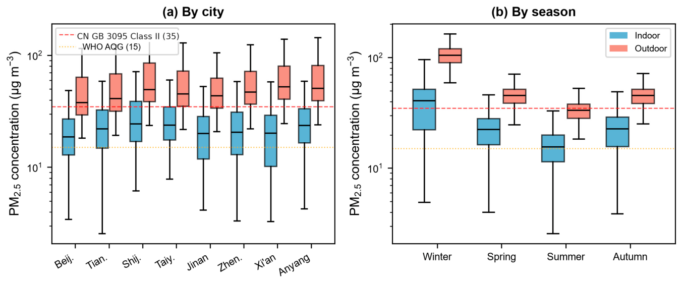
Across all 48 residences and four seasons, mean indoor PM2.5 was 24.9 μg m−3 (median 21.8, SD 14.7, range 2.1–354.6) and mean outdoor PM2.5 was 57.6 μg m−3 (median 45.9, SD 41.2); the overall median I/O ratio was 0.47 (IQR 0.29–0.71). Figure 2 shows distributions by site and season. City comparisons use residence-level annual means rather than hourly records: a Kruskal–Wallis test on the 48 residence means gave H = 31.6 (p < 0.001)—substantially smaller than the value obtained by treating hours as independent, because the latter reflects pseudo-replication. Site C3 recorded the highest mean indoor concentration (29.7 μg m−3) and C5 the lowest (20.9 μg m−3). Residence-level descriptive statistics (n = 6 homes per site) are given in Table 4; error bars/box widths throughout represent the inter-residence distribution (SD/IQR as labelled), and every comparison reports its sample size.
Seasonal variation was pronounced (Figure 2b). Because each residence was measured in all four seasons, seasonal contrasts are repeated-measures and were tested with the Friedman test on residence seasonal means (χ2 = 89.4, p < 0.001). Winter showed the highest indoor (38.5 μg m−3) and outdoor (105.6 μg m−3) means, ≈2.4 and 3.1 times summer values (15.8 and 33.5 μg m−3); spring/autumn were intermediate (22.5/22.7). The indoor–outdoor gradient was compressed in winter (I/O = 0.36) relative to summer (0.47), consistent with tighter window closure during polluted winter periods.
The I/O ratio varied within and between sites (0.38 at C1 vs. 0.55 at C3). Among the seven rural residences, all using coal for cooking/heating, indoor PM2.5 was comparable to urban homes (25.1 vs. 24.8 μg m−3) but the I/O ratio was slightly higher (0.52 vs. 0.47), consistent with solid-fuel use and leakier envelopes [5].

3.2. Diurnal Patterns

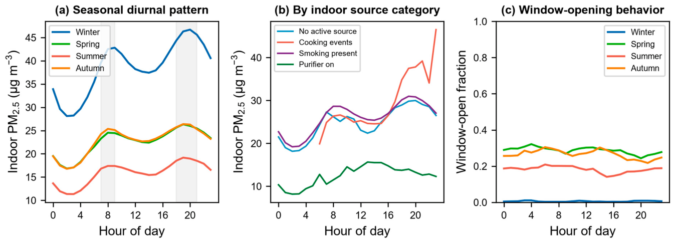
Figure 3 shows a bimodal diurnal pattern in all seasons, with morning (07:00–09:00) and evening (18:00–21:00) peaks coinciding with cooking and rush-hour traffic; the evening peak was highest in winter (48.6 μg m−3). Residences with smoking had the highest all-day mean (41.2 μg m−3), followed by cooking-event hours (28.6), while residences with operating purifiers maintained the lowest levels (12.8). Window-open fraction peaked in spring/autumn daytime (up to 0.55), was low in winter (<0.08) and moderate in summer (0.25–0.40).

3.3. Indoor–Outdoor Relationships and Infiltration Factors

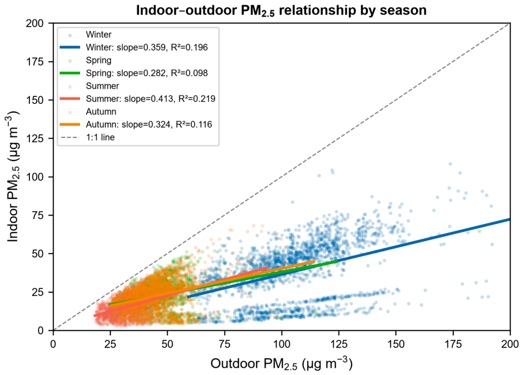
Figure 4 shows C_in vs. C_out by season. The population-averaged slope (an aggregate infiltration proxy) was 0.359 (winter), 0.282 (spring), 0.413 (summer) and 0.324 (autumn), with modest R2 (0.10–0.22) because indoor source events are included; on no-source hours the median building-level R2 was 0.78 (range 0.10–0.92).
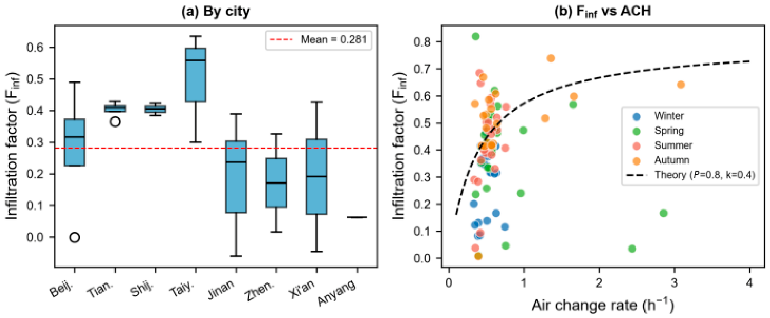
Building-specific F_inf from no-source periods ranged from −0.06 to 0.63 (mean 0.28 ± 0.15; Figure 5a); negative values occurred in three homes with continuously running high-capacity purifiers that decoupled indoor from outdoor air. F_inf correlated with estimated ACH (Pearson r = 0.62, p < 0.001), consistent with F_inf = P·a/(a + k) (Figure 5b). The mass-balance analysis ESTIMATED a median deposition rate k of 0.53 h−1 (IQR 0.35–0.76) and a median estimated ACH of 0.52 h−1 across buildings/seasons (window-open periods > 2 h−1); these are model-derived quantities subject to the ≈±20% estimated-ACH uncertainty in Section 2.5, not directly measured values. Seasonal mass-balance parameters are summarised in Table 5.
Table 5. Seasonal mass-balance parameters (penetration, deposition, estimated ACH, infiltration, no-source R2).
Seasonp (Penetration)k (h−1)Estimated ACH (h−1)F_infR2
Winter0.80 *0.67 (0.55–1.89)0.510.34 (0.17–0.40)0.84
Spring0.80 *0.58 (0.39–0.90)0.570.41 (0.24–0.48)0.39
Summer0.80 *0.44 (0.33–0.60)0.520.41 (0.38–0.50)0.42
Autumn0.80 *0.39 (0.23–0.52)0.530.48 (0.41–0.57)0.44
* p = 0.80 is an assumed base value; the p = 0.6/0.8/1.0 sensitivity in Table 6 spans the resulting uncertainty.
Table 6. Primary linear mixed-effects model of log(indoor PM2.5): fixed effects with 95% CI; residence random intercept (τ = 0.213), AR(1) residuals; marginal R2 = 0.71, conditional R2 = 0.91.
PredictorβSEtp95% CI Low95% CI High
log(Outdoor PM2.5)0.8720.04121.27<0.0010.790.954
Window-open fraction0.5480.0589.45<0.0010.4320.664
Cooking event0.0460.0123.83<0.0010.0220.07
Smoking present0.0290.0390.740.462−0.0490.107
Air purifier (owned)−0.2210.044−5.02<0.001−0.309−0.133
Purifier-on fraction−0.9020.061−14.79<0.001−1.024−0.78
Temperature0.00040.0010.40.690−0.0010.002
Relative humidity−0.0020.001−2.050.041−0.003−0.0001
Wind speed−0.0020.003−0.620.536−0.0070.003
Building age−0.00030.004−0.080.936−0.0090.008
Envelope airtightness (n50)0.1870.1071.750.082−0.0270.401
Floor level−0.0020.002−0.760.448−0.0060.002
Occupants−0.020.012−1.670.096−0.0440.004
Range hood present−0.0350.033−1.060.290−0.1010.031
Rural location0.030.0440.680.497−0.0580.118
Window-open × log(Outdoor)0.1180.0472.510.0120.0240.212
Purifier-on × log(Outdoor)−0.0940.04−2.350.021−0.174−0.014

3.4. Multivariable Determinants: Mixed-Effects Model and Robustness

The residence random-intercept variance was τ = 0.213 and the residual SD 0.298, giving an intra-class correlation of 0.34: about one third of residual variance lies BETWEEN residences, confirming that hourly records are strongly clustered and that a mixed-effects model is required. The primary LMM achieved marginal R2 = 0.71 (fixed effects) and conditional R2 = 0.91 (fixed + random intercepts); leave-one-residence-out cross-validation gave out-of-sample R2 = 0.7, and the original single-level OLS fit reported R2 = 0.879. The smaller marginal/cross-validated R2 is the honest predictive value of the measured covariates; the gap to conditional R2 reflects stable between-residence differences captured by the random intercept. Residual diagnostics (Q–Q plot, residuals vs. fitted, scale-location) showed approximate normality and no systematic heteroscedasticity; all VIF were <3.5.
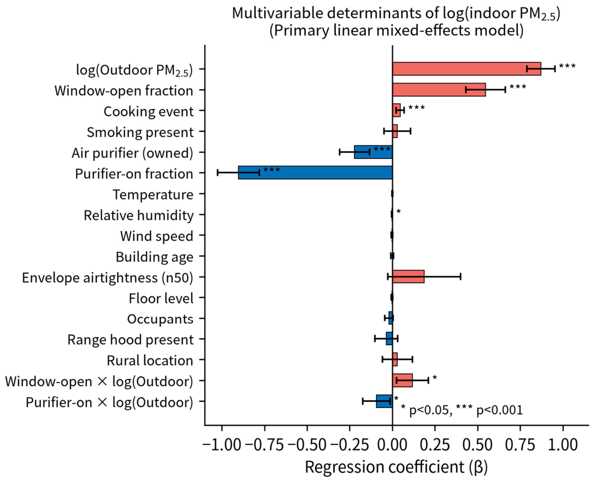
Fixed-effect estimates with Satterthwaite-based 95% confidence intervals are given in Table 6. On the log scale, a 10% higher outdoor PM2.5 was associated with an 8.7% higher indoor concentration (β = 0.872); fully open vs. closed windows with 73.0% higher indoor PM2.5 (β = 0.548); and an active cooking event with 4.7% higher hourly PM2.5 (β = 0.046). Purifier ownership was associated with 19.8% lower indoor PM2.5 (β = −0.221) and the fraction of time a purifier ran with 59.4% lower indoor PM2.5 (β = −0.902). These are observational ASSOCIATIONS adjusted for the listed covariates, not causal effects. Smoking, temperature, wind, building age, floor, occupants, hood ownership and rural location were not independently significant after adjustment. The two pre-specified interactions were significant: window opening amplified the outdoor–indoor transmission (β = 0.118, p = 0.012), whereas purifier operation attenuated it more as outdoor pollution rose (β = −0.094, p = 0.021) (Figure 6).
Robustness to estimator and aggregation. Table 7 compares the key coefficients under four specifications: conventional cluster-robust OLS (CR1), finite-cluster CR2 OLS, the hourly LMM and a daily aggregated LMM (1344 scheduled residence-days, 48 clusters). Coefficients and significance are stable; CR2 standard errors are slightly larger than CR1 (as expected with 48 clusters), and daily aggregation—which removes within-day serial dependence—changes point estimates by <0.07. Restricting cooking events to the 68% independently diary-confirmed events gave β = 0.044 (vs. 0.046), so the results do not depend on algorithm-defined events.
Behavioural Feedback and Lagged Effects: Because occupants switch purifiers on when outdoor pollution rises, purifier use is a time-varying behaviour correlated with outdoor PM2.5 (r = 0.38). A lag-1 h purifier variable remained strongly associated with lower indoor PM2.5 (β = −0.873, SE = 0.068, p < 0.001), while lagged outdoor PM2.5 predicted subsequent purifier activation (β = 0.31, p < 0.001), confirming reactive use. The purifier association therefore persists after acknowledging this feedback, but residual time-varying confounding cannot be excluded and the estimate should not be read as the effect of a randomised intervention.

3.5. Estimated Outdoor and Indoor Contributions

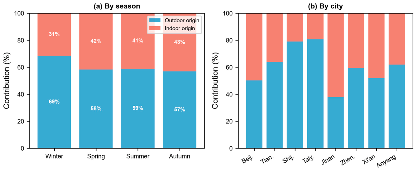
We deliberately describe this analysis as ESTIMATED OUTDOOR/INDOOR CONTRIBUTIONS rather than chemical source apportionment: no speciation or size-resolved data were collected, so specific sources (e.g., traffic, combustion) cannot be identified. At the base penetration p = 0.8 the estimated outdoor contribution was 60.7% (indoor-generated 39.3%), highest in winter (68.5%) and similar across the other seasons (59.6/59.0/61.2%); across sites it ranged from 37.8% (C5) to 80.8% (C4). Because p is assumed rather than measured, Table 8 propagates this assumption: varying p from 0.6 to 1.0 moves the mean outdoor contribution from 54.8% to 66.3% and mean F_inf from 0.23 to 0.33. The qualitative conclusion—outdoor PM2.5 is the dominant but not sole driver, with a larger role in winter—is unchanged throughout this range (Figure 7).
Indoor-generated PM2.5 was dominated by cooking. Cooking occupied 12.4% of monitored hours but contributed 33.8% of the indoor mass above the non-cooking baseline (a single, consistent definition; the 33.3% figure in the earlier draft was a transcription error and has been removed throughout). Mean cooking-event peaks were 68.5 μg m−3, and residences with regular smokers had 1.65-fold higher indoor PM2.5 than non-smoking homes.

3.6. Correlation Structure

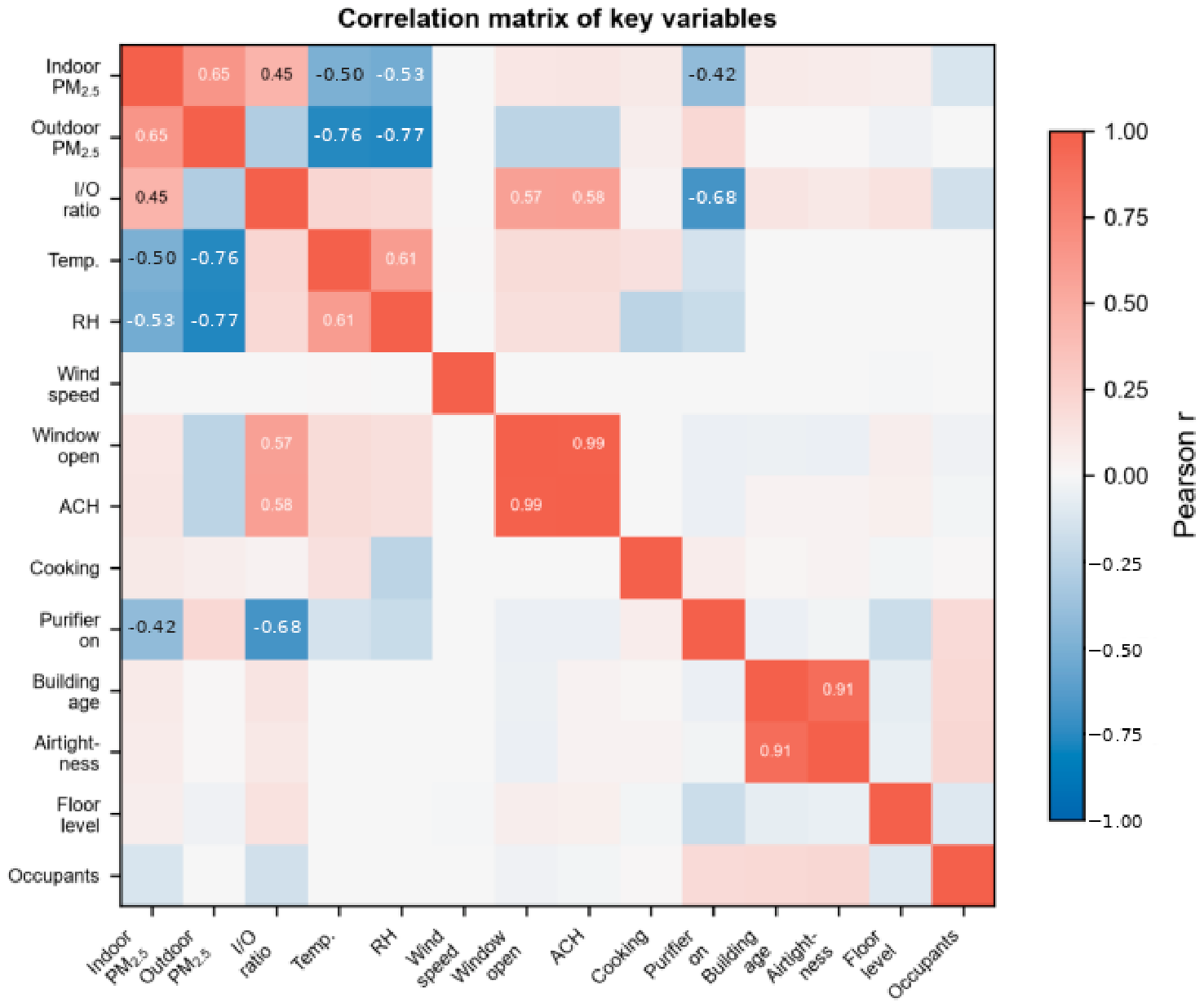
Figure 8 shows pairwise correlations. Indoor PM2.5 correlated most strongly with outdoor PM2.5 (r = 0.81), window-open fraction (r = 0.59), purifier-on fraction (r = −0.56) and cooking (r = 0.38). Purifier-on fraction correlated positively with outdoor PM2.5 (r = 0.38), i.e., purifiers were used more on polluted days—again illustrating the behavioural feedback addressed in Section 3.4. Estimated ACH and n50 correlated weakly positively with indoor PM2.5 (r = 0.31/0.28), while RH showed a weak negative association (r = −0.22).

3.7. Guideline Exceedance and Estimated Residential Intake

We quantified the fraction of occupied hours above the WHO 2021 24 h Air Quality Guideline (15 μg m−3) and the Chinese ambient Class II limit (35 μg m−3, GB 3095-2012); for reference, the Chinese indoor standard GB/T 18883-2022 sets a 24 h indoor limit of 50 μg m−3 [36]. Across all residences/seasons, the WHO guideline was exceeded during 72.4% of monitored hours and the 35 μg m−3 limit during 20.2%; in winter, the 35 μg m−3 limit was exceeded during 60.7% of hours versus 0.5% in summer (Table 9). Assuming a breathing rate of 0.6 m3 h−1 and 16 h day−1 at home, mean daily residential PM2.5 intake was estimated at 239 μg day−1 (201 at C5 to 285 at C3). These are exposure-model estimates intended for relative comparison across sites, not individual dose measurements.

4. Discussion

4.1. Outdoor Pollution and Seasonal Infiltration

The dominant association of indoor PM2.5 with outdoor PM2.5 (β = 0.872; r = 0.81) and the estimated ≈60.7% outdoor contribution agree with the broader literature [6,20] and with the recent twelve-city Chinese survey [35]. The lower winter F_inf (≈0.34 at p = 0.8) relative to summer (≈0.41) is consistent with Lunderberg et al. [6], who reported roughly halved infiltration in winter across most climate zones. Two mechanisms plausibly operate here: near-universal window closure during district heating, which lowers the estimated ACH; and enhanced deposition of particles infiltrating through cold envelope leaks under large indoor–outdoor temperature differences (ΔT > 20 °C) [25]. This seasonal buffering is protective during the most polluted period, and the trend toward tighter, energy-retrofitted envelopes may co-reduce outdoor-particle infiltration [25]; without adequate mechanical ventilation, however, tighter envelopes can increase exposure to indoor-generated particles, consistent with the larger estimated indoor contribution in summer [9,26].

4.2. Building Envelope and Ventilation Behaviour

Window-opening was the second-strongest adjustable correlate (β = 0.548; +73.0% when fully open vs. closed), and the significant window × outdoor interaction (β = 0.118) shows that opening windows transmits outdoor PM most strongly on polluted days. Envelope airtightness n50 was borderline (β = 0.187, p = 0.082): leakier homes tended toward higher indoor PM, in line with the envelope literature [27]. Because window sensors record only open/closed and half of the ACH values are estimated (±20%), these coefficients describe ventilation behaviour rather than precise airflow effects; future work should combine tracer-gas ACH, opening-area and flow measurements.

4.3. Indoor Sources and the Role of Air Purifiers: Association, Not Causation

Cooking accounted for the largest estimated indoor-generated contribution among the monitored source categories: it occupied 12.4% of monitored hours but contributed 33.8% of the mass above the non-cooking baseline, and the diary-only sensitivity gave essentially the same coefficient (0.044 vs. 0.046), supporting the result despite the difficulty of identifying events independently of the PM trace [23]. Range-hood OWNERSHIP was not significant after adjustment (β = −0.035, p = 0.290), which we interpret as the well-documented gap between device availability and actual use: hoods are operated during only a minority of cooking events in many homes, and cooktop/hood design strongly affects capture [21,24,31].
We are careful to frame purifier findings as observational associations. Purifier-on fraction was associated with 59.4% lower indoor PM2.5 (β = −0.902) and ownership with 19.8% lower levels, magnitudes consistent with intervention studies reporting 22–92% reductions [12,13,14,15,16]; however, purifier use was positively correlated with outdoor PM2.5 (r = 0.38) and lagged outdoor PM predicted subsequent purifier activation (β = 0.31), demonstrating reactive, time-varying behaviour. The mixed model adjusts for measured contemporaneous confounders and the lagged analysis shows that the association persists, but residual confounding and reverse causality cannot be excluded in an observational design; quasi-experimental or randomised designs would be needed for causal effect estimates [13]. The significant purifier × outdoor interaction (β = −0.094) suggests purifiers confer greater relative protection as outdoor pollution rises.

4.4. Geographic and Seasonal Generalisability

The eight sites span annual ambient means of roughly 33–72 μg m−3 and diverse building stocks. Using residence-level inference, site and season remained significant but the effect sizes were far smaller than those obtained by treating hourly records as independent (Kruskal–Wallis H = 31.6 and Friedman χ2 = 89.4 on residence means), illustrating how pseudo-replication inflates such tests. Rural coal-using homes had somewhat higher I/O ratios (0.52 vs. 0.47) but similar mean indoor concentrations; this is broadly comparable to, though less extreme than, concentrations reported for solid-fuel rural households elsewhere in Northern China [5,32].

4.5. Strengths and Limitations

Strengths include 48 independent residences across eight climatically diverse cities (a larger independent sample than most prior Chinese residential studies, which commonly cover 4–12 homes [11,19]), four-season paired monitoring, gravimetric calibration, and—most importantly—inference anchored to the residence via a random-intercept/AR(1) mixed model with CR2 finite-cluster checks, daily aggregation and penetration-factor sensitivity. We deliberately avoid describing this campaign as the ‘largest’; rather, it broadens the independent-unit and geographic basis for inference.
Limitations remain. First, the effective independent sample is 48 residences (not 31,094 valid hours); confidence intervals are correctly wider than in the original single-level analysis and extrapolation beyond Northern China’s cold zone should be cautious. Second, no chemical speciation or size-resolved data were collected, so we estimate aggregate outdoor/indoor contributions and cannot identify specific sources. Third, the penetration factor is assumed (p = 0.8) and half of the ACH values are estimated; the reported p = 0.6–1.0 and ±20% estimated-ACH ranges bound—but do not eliminate—this uncertainty. Fourth, window state is binary and purifier use is self-/sensor-reported behaviour, leaving residual time-varying confounding. Fifth, one calendar year and a stratified (not random) residential sample limit temporal and population representativeness.

5. Conclusions

Based on paired four-season monitoring of 48 residences across eight Northern Chinese cities and a residence-level linear mixed-effects analysis, this study reaches the following key findings, each tied directly to the reported results:
(1)
Indoor PM2.5 averaged 24.9 μg m−3 with strong seasonality (winter 38.5 vs. summer 15.8 μg m−3) and between-site variation (20.9 at C5 to 29.7 μg m−3 at C3); the median I/O ratio was 0.47 and the estimated mean infiltration factor 0.28 ± 0.15.
(2)
After simultaneous adjustment and correct clustering at the residence (marginal R2 = 0.71, conditional R2 = 0.91), outdoor PM2.5 (β = 0.872), window-open fraction (β = 0.548) and cooking (β = 0.046) were positively, and purifier operation (β = −0.902) was negatively, associated with indoor PM2.5; smoking, building age, floor and hood ownership were not independently significant. Results were stable under CR2 finite-cluster inference, daily aggregation and diary-only cooking definitions.
(3)
Estimated outdoor contribution was 60.7% (range 54.8–66.3% across p = 0.6–1.0), peaking in winter (68.5%); cooking occupied 12.4% of hours yet contributed 33.8% of indoor mass above baseline, with cooking accounting for the largest estimated indoor-generated contribution among the monitored source categories.
(4)
Continuous purifier operation was associated with 59.4% lower indoor PM2.5 (and ownership with 19.8%), with stronger relative protection on polluted days; because use is reactive (r = 0.38 with outdoor PM), this is an adjusted association rather than a causal effect, and correct, sustained operation mattered more than ownership.
Practical implication: continued reduction in ambient PM2.5 remains the primary long-term measure, while informed window management on polluted days, reliable kitchen exhaust during cooking, and correct air-purifier operation offer near-term residential exposure reductions. These recommendations are robust to the estimator, temporal aggregation and penetration-factor assumptions examined here.

Author Contributions

Conceptualization, W.L.; methodology, W.L.; software, W.L.; validation, W.L. and Q.H.; formal analysis, W.L.; investigation, W.L. and Q.H.; resources, W.L.; data curation, W.L.; writing—original draft preparation, W.L.; writing—review and editing, W.L. and Q.H.; visualisation, W.L.; supervision, Q.H.; project administration, W.L.; funding acquisition, W.L. All authors have read and agreed to the published version of the manuscript.

Funding

This research was funded by Anyang Normal University (Research grant No. 192179524001).

Institutional Review Board Statement

Ethical review and approval were granted/waived by the Research Ethics Committee of Anyang Normal University (reference AYNU-REC-2024-118), because the study involved environmental monitoring only and collected no identifiable, sensitive personal data, medical information or human biological samples, and posed no foreseeable risk to participants.

Informed Consent Statement

Informed verbal consent was obtained from all participating households prior to instrument deployment and data collection.

Data Availability Statement

The data presented in this study are available from the corresponding author upon reasonable request.

Conflicts of Interest

The authors declare no conflicts of interest.

Abbreviations

PM2.5Fine particulate matter (aerodynamic diameter ≤ 2.5 um)
I/OIndoor-to-outdoor concentration ratio
F_infInfiltration factor
ACHAir change rate (h−1), model-estimated in this study (referred to as “estimated ACH”)
HEPAHigh-efficiency particulate air (filter)
LMMLinear mixed-effects model
OLSOrdinary least squares
CR1/CR2Cluster-robust variance estimator, conventional/bias-reduced (CR2)
REMLRestricted maximum likelihood
VIFVariance inflation factor
ICCIntra-class correlation coefficient
SD/SE/CIStandard deviation/error/confidence interval
IQRInterquartile range
WHO AQGWorld Health Organization Air Quality Guideline
GBGuobiao (Chinese national standard)
RHRelative humidity
PMFPositive matrix factorization
CVCross-validation

References

  1. Yu, W.; Xu, R.; Ye, T.; Abramson, M.J.; Morawska, L.; Jalaludin, B.; Johnston, F.H.; Henderson, S.B.; Knibbs, L.D.; Morgan, G.G.; et al. Estimates of global mortality burden associated with short-term exposure to fine particulate matter (PM2.5). Lancet Planet. Health 2024, 8, e146–e155. [Google Scholar] [CrossRef] [Scilit] [PubMed]
  2. Huang, W.; Zhou, Y.; Chen, X.; Zeng, X.; Knibbs, L.D.; Zhang, Y.; Jalaludin, B.; Dharmage, S.C.; Morawska, L.; Guo, Y.; et al. Individual and joint associations of long-term exposure to air pollutants and cardiopulmonary mortality: A 22-year cohort study in Northern China. Lancet Reg. Health West. Pac. 2023, 36, 100776. [Google Scholar] [CrossRef] [Scilit] [PubMed]
  3. Saraga, D.; Duarte, R.M.; Manousakas, M.; Maggos, T.; Tobler, A.; Querol, X. From outdoor to indoor air pollution source apportionment: Answers to ten challenging questions. TrAC Trends Anal. Chem. 2024, 178, 117821. [Google Scholar] [CrossRef] [Scilit]
  4. Bousiotis, D.; Beddows, D.; Dall’Osto, M.; Harrison, R.M.; Pope, F.D. Evaluating the use of low-cost sensors to quantify PM10 and PM2.5 source apportionment indoors. Environ. Int. 2023, 177, 107918. [Google Scholar] [CrossRef] [Scilit] [PubMed]
  5. Xie, C.; Lin, B.; Chen, Y.; Xu, X. Characteristics of indoor heating sources and PM2.5 pollution in rural residences of Qingdao, China. Buildings 2023, 13, 1980. [Google Scholar] [CrossRef] [Scilit]
  6. Lunderberg, D.M.; Liang, Y.; Singer, B.C.; Apte, J.S.; Nazaroff, W.W.; Goldstein, A.H. Assessing residential PM2.5 concentrations and infiltration factors with high spatiotemporal resolution using crowdsourced sensors. Proc. Natl. Acad. Sci. USA 2024, 120, e2308832120. [Google Scholar] [CrossRef] [Scilit] [PubMed]
  7. Hou, W.; Wang, J.; Hu, R.; Chen, Y.; Shi, J.; Lin, X.; Qin, Y.; Zhang, P.; Du, W.; Tao, S. Systematically quantifying the dynamic characteristics of PM2.5 in multiple indoor environments in a plateau city: Implication for internal contribution. Environ. Int. 2024, 186, 108641. [Google Scholar] [CrossRef] [Scilit] [PubMed]
  8. Lin, B.; Xie, C.; Chen, Y.; Xu, X. Natural ventilation potential of residential buildings in China considering the combined effect of indoor and outdoor air pollution. Buildings 2024, 14, 363. [Google Scholar] [CrossRef] [Scilit]
  9. Wang, Z.; Hou, J.; Fu, J.; Tian, Z.; Feng, S.; Kosonen, R.; Sun, Y. Health-demand ventilation control strategy in northern Chinese homes: How much ventilation do we need to protect occupants’ health? Front. Built Environ. 2025, 11, 1510965. [Google Scholar] [CrossRef] [Scilit]
  10. Abdalla, T.; Peng, C. Spatiotemporal variability of PM2.5 infiltrations in higher education buildings: A multizone air-thermal co-simulation analysis. J. Build. Eng. 2025, 111, 113473. [Google Scholar] [CrossRef] [Scilit]
  11. Lowther, S.D.; Jones, R.; Dimitroulopoulou, S.; Font, A. Setting the baseline for indoor air quality: Measuring and understanding PM2.5 in UK homes. Environ. Sci. Adv. 2023, 2, 323–337. [Google Scholar] [CrossRef] [Scilit]
  12. Edwards, L.; Wilkinson, P.; Rutter, G.; Iverson, L.; Milojevic, A. Impact of mitigation measures to improve home indoor air quality in Kathmandu, Nepal. Environ. Res. Health 2023, 1, 025004. [Google Scholar] [CrossRef] [Scilit]
  13. Klaver, Z.M.; Crane, R.C.; Ziemba, R.A.; Bard, R.L.; Adar, S.D.; Brook, R.D.; Morishita, M. Reduction of outdoor and indoor PM2.5 source contributions via portable air filtration systems in a senior residential facility in Detroit, Michigan. Toxics 2023, 11, 1019. [Google Scholar] [CrossRef] [Scilit] [PubMed]
  14. Lu, F.T.; Laumbach, R.J.; Legard, A.; Myers, N.T.; Black, K.G.; Ohman-Strickland, P.; Alimokhtari, S.; De Resende, A.; Calderon, L.; Mainelis, G.; et al. Real-world effectiveness of portable air cleaners in reducing home particulate matter concentrations. Aerosol Air Qual. Res. 2024, 24, 230202. [Google Scholar] [CrossRef] [Scilit] [PubMed]
  15. McIntyre, A.M.; Scammell, M.K.; Kinney, P.L.; Khosla, K.; Benton, L.; Bongiovanni, R.; McCannon, J.; Milando, C.W. Portable air cleaner usage and particulate matter exposure reduction in an environmental justice community: A pilot study. Environ. Health Insights 2024, 18, 11786302241258587. [Google Scholar] [CrossRef] [Scilit] [PubMed]
  16. Singhsmith, K.; Sprague Martinez, L.; Eliasziw, M.; Lerman Ginzburg, S.; Hudda, N.; Betz, G.M.; Gurcan, A.; Vazquez-Dodero, T.; Mertl, A.; Goldstein-Gelb, W.; et al. Reaction to at-home air purifiers installed to reduce traffic-related air pollution in near-highway residences. Trials 2024, 25, 514. [Google Scholar] [CrossRef] [Scilit] [PubMed]
  17. Ding, E.; Giri, A.; Gaillard, A.; Bonn, D.; Bluyssen, P.M. Using mobile air cleaners in school classrooms for aerosol removal: Which, where and how. Indoor Built Environ. 2024, 33, 1964–1987. [Google Scholar] [CrossRef] [Scilit]
  18. Jia, L.; Ge, J.; Wang, Z.; Jin, W.; Wang, C.; Dong, Z.; Wang, C.; Wang, R. Synergistic impact on indoor air quality: The combined use of air conditioners, air purifiers, and fresh air systems. Buildings 2024, 14, 1562. [Google Scholar] [CrossRef] [Scilit]
  19. Wenner, M.M.; Ries-Roncalli, A.; Whalen, M.C.R.; Jing, P. The relationship between indoor and outdoor fine particulate matter in a high-rise building in Chicago monitored by PurpleAir sensors. Sensors 2024, 24, 2493. [Google Scholar] [CrossRef] [Scilit] [PubMed]
  20. Zhao, J.; Fung, P.L.; Zaidan, M.A.; Wehner, B.; Weinhold, K.; Wiedensohler, A.; Hussein, T. Indoor black carbon concentrations and their sources in residential environments: Validation of an input-adaptive proxy model. Aerosol Air Qual. Res. 2024, 24, 230228. [Google Scholar] [CrossRef] [Scilit]
  21. Pantelic, J.; Tang, M.; Byun, K.; Knobloch, Y.; Son, Y.J. Comparison of cooking emissions mitigation between automated and manually operated air quality interventions in one-bedroom apartments. Sci. Rep. 2024, 14, 19435. [Google Scholar] [CrossRef] [Scilit] [PubMed]
  22. Tang, R.; Pfang, C. Indoor particulate matter (PM) from cooking in UK students’ studio flats and associated intervention strategies: Evaluation of cooking methods, PM concentrations and personal exposures using low-cost sensors. Environ. Sci. Atmos. 2023, 3, 537–551. [Google Scholar] [CrossRef] [Scilit]
  23. Shi, S.; Yang, J.; Liang, Y. Indoor distribution and personal exposure of cooking-generated PM2.5 in rural residences of China: A multizone model study. Build. Simul. 2023, 16, 1299–1315. [Google Scholar] [CrossRef] [Scilit]
  24. Li, J.; Zhao, H.; Russell, M.L.; Delp, W.W.; Johnson, A.; Tang, X.; Walker, I.S.; Singer, B.C. Air pollutant exposure concentrations from cooking a meal with a gas or induction cooktop and the effectiveness of two recirculating range hoods with filters. Indoor Environ. 2024, 1, 100047. [Google Scholar] [CrossRef] [Scilit]
  25. Lozinsky, C.H.; Casquero-Modrego, N.; Walker, I.S. The health and indoor environmental quality impacts of residential building envelope retrofits: A literature review. Build. Environ. 2025, 270, 112568. [Google Scholar] [CrossRef] [Scilit]
  26. Ferdyngrygierek, J.; Grygierek, K. Ventilation methods for improving the indoor air quality and energy efficiency of multi-family buildings in Central Europe. Energies 2024, 17, 2232. [Google Scholar] [CrossRef] [Scilit]
  27. Zhang, C.; Yu, Z.; Zhu, Q.; Shi, H.; Yu, Z.; Xu, X. Air-permeable building envelopes for building ventilation and heat recovery: Research progress and future perspectives. Buildings 2024, 14, 42. [Google Scholar] [CrossRef] [Scilit]
  28. Li, T.; Zhang, Y.; Jiang, N.; Du, H.; Chen, C.; Wang, J.; Li, Q.; Feng, D.; Shi, X. Ambient fine particulate matter and cardiopulmonary health risks in China. Chin. Med. J. 2023, 136, 1025–1034. [Google Scholar] [CrossRef] [Scilit] [PubMed]
  29. Jiang, S.; Tong, X.; Yu, K.; Yin, P.; Shi, S.; Meng, X.; Chen, R.; Zhou, M.; Kan, H.; Niu, Y.; et al. Ambient particulate matter and chronic obstructive pulmonary disease mortality: A nationwide, individual-level, case-crossover study in China. eBioMedicine 2024, 104, 105168. [Google Scholar] [CrossRef] [Scilit] [PubMed]
  30. Bai, Y.; Chen, L.; Feng, Z.; Zhu, J.; Gu, Y.; Li, K.; Liao, H. Historical and future health burden attributable to PM2.5 exposure in China. Atmos. Environ. 2024, 322, 120363. [Google Scholar] [CrossRef] [Scilit]
  31. Zhao, H.; Walker, I.S.; Delp, W.W.; Singer, B.C. Factors impacting range hood use in California houses and low-income apartments. Int. J. Environ. Res. Public Health 2020, 17, 8870. [Google Scholar] [CrossRef] [Scilit] [PubMed]
  32. Chan, K.H.; Xia, X.; Ho, K.-F.; Guo, Y.; Kurmi, O.P.; Du, H.; Bennett, D.A.; Bian, Z.; Kan, H.; McDonnell, J. Regional and seasonal variations in household and personal exposures to air pollution in one urban and two rural Chinese communities: A pilot study to collect time-resolved data using static and wearable devices. Environ. Int. 2021, 146, 106217. [Google Scholar] [CrossRef] [Scilit] [PubMed]
  33. Pustejovsky, J.E.; Tipton, E. Small-sample methods for cluster-robust variance estimation and hypothesis testing in fixed effects models. J. Bus. Econ. Stat. 2018, 36, 672–683. [Google Scholar] [CrossRef] [Scilit]
  34. Nakagawa, S.; Johnson, P.C.D.; Schielzeth, H. The coefficient of determination R2 and intra-class correlation coefficient from generalized linear mixed-effects models revisited and expanded. J. R. Soc. Interface 2017, 14, 20170213. [Google Scholar] [CrossRef] [Scilit] [PubMed]
  35. Cao, Y.; Zhang, X.; Zhang, W.; Jiang, L.; Yang, Y.; Du, H.; Fan, L.; Wang, X. PM2.5 characteristics and influencing factors in residential homes across 12 cities in China. J. Environ. Hyg. 2024, 14, 233–241. [Google Scholar]
  36. GB/T 18883-2022; Indoor Air Quality Standard. Standardization Administration of China: Beijing, China; National Health Commission of China: Beijing, China; Standards Press of China: Beijing, China, 2022. (In Chinese)
  37. GB 50176-2016; Code for Thermal Design of Civil Building. China Architecture & Building Press: Beijing, China, 2016.
  38. GB 3095-2012; Ambient Air Quality Standards. China Environmental Science Press: Beijing, China, 2012.
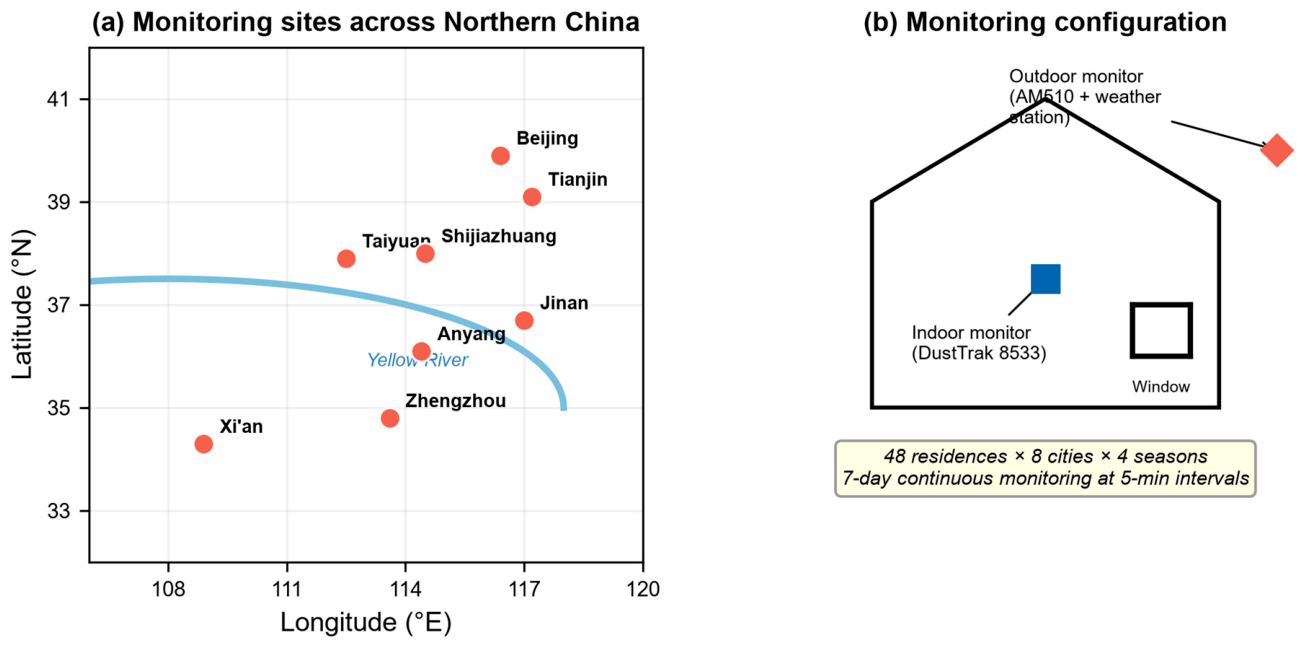
Figure 1. (a) Locations of the eight study sites (C1–C8) in Northern China; (b) schematic of the paired indoor–outdoor monitoring setup.
Atmosphere 17 00874 g001
Figure 2. Distribution of indoor (blue) and outdoor (red) PM2.5 (a) by site code and (b) by season. Boxes show median and IQR; whiskers show 10th–90th percentiles (n homes = 48; n hours shown in Table 4). The dashed 15 μg m−3 line is the WHO 2021 24 h Air Quality Guideline, whereas the 35 μg m−3 dotted line is the Chinese ambient Class II limit (GB 3095-2012 [38]), NOT a WHO value. Log y-axis.
Atmosphere 17 00874 g002
Figure 3. Diurnal patterns: (a) indoor PM2.5 by season (shaded bands = meal-preparation hours); (b) indoor PM2.5 by indoor-source category; (c) window-open fraction by season. Bands/lines are residence-level means; n = 48 residences.
Atmosphere 17 00874 g003
Figure 4. Indoor vs. outdoor PM2.5 by season with regression lines; dashed 1:1 line for reference (n ≈ 7725–7814 valid hours per season).
Atmosphere 17 00874 g004
Figure 5. (a) Building-specific F_inf by site (dashed = grand mean); (b) F_inf vs. estimated ACH coloured by season; dashed curve = theoretical F_inf = P·a/(a + k) at p = 0.8, k = 0.4 h−1.
Atmosphere 17 00874 g005
Figure 6. Standardised fixed-effect coefficients (95% CI) from the primary mixed-effects model. Error bars are 95% confidence intervals based on Satterthwaite degrees of freedom (not the conventional cluster-robust intervals of the original OLS); n = 48 residence clusters, 31,094 valid hourly observations.
Atmosphere 17 00874 g006
Figure 7. Estimated contributions of outdoor and indoor sources to indoor PM2.5 by (a) season and (b) site. These are mass-balance estimates, not chemical source apportionment; whiskers span the p = 0.6–1.0 sensitivity.
Atmosphere 17 00874 g007
Figure 8. Pearson correlation matrix of indoor/outdoor PM2.5, behavioural, building and meteorological variables (hourly).
Atmosphere 17 00874 g008
Table 1. Site codes and characteristics (six residences per site).
CodeCitySite Description
C1BeijingMegacity, strict controls
C2TianjinMegacity, coastal
C3ShijiazhuangIndustrial, historically high PM
C4TaiyuanCoal/industrial inland
C5JinanProvincial capital
C6ZhengzhouProvincial capital
C7Xi’anNorth-west basin
C8AnyangMedium industrial Henan
Table 2. Summary of building and household characteristics (n = 48).
CharacteristicCategoryn%
Building age≤10 years1429.2
11–20 years2041.7
>20 years1429.2
Floor area<80 m21225.0
80–110 m22450.0
>110 m21225.0
Heating typeDistrict heating2245.8
Natural gas1225.0
Electric heat pump714.6
Coal (rural)714.6
Kitchen typeClosed3470.8
Open1429.2
Range hoodPresent4185.4
Air purifierPresent1735.4
SmokingNone2654.2
Occasional1531.2
Regular714.6
LocationUrban4185.4
Rural714.6
Table 3. Residence-level data coverage and missingness. Each residence was scheduled for 28 monitoring days (7 per season). For 48 residences, 48 × 7 × 24 = 8064 h were scheduled in each season and 48 × 28 × 24 = 32,256 h across the full campaign; after quality control, 31,094 valid hours remained, so valid hours cannot exceed scheduled hours in any season.
PeriodScheduled HoursValid HoursMissing %
Winter (heating)806478143.1%
Spring transition806477254.2%
Summer806477573.8%
Autumn transition806477983.3%
Total32,25631,0943.6%
Table 4. Residence-level descriptive statistics of indoor/outdoor PM2.5 by site (six residences per site). Each site was scheduled for 4032 h (6 residences × 28 d × 24 h); site valid-hour totals after quality control are listed in the final column and are all below this ceiling.
SiteIndoor Mean ± SDIndoor MedianIndoor P95Outdoor MeanOutdoor MedianI/O MedianValid Hours
C1 Beijing21.5 ± 11.918.744.749.238.00.503890
C2 Tianjin24.9 ± 13.422.150.852.541.10.503876
C3 Shijiazhuang29.7 ± 17.124.564.664.849.50.503902
C4 Taiyuan28.1 ± 14.323.961.356.645.20.503884
C5 Jinan20.9 ± 10.520.139.651.943.60.403895
C6 Zhengzhou23.7 ± 14.420.651.558.047.20.503871
C7 Xi’an23.2 ± 16.620.357.664.152.50.403888
C8 Anyang27.1 ± 15.523.859.264.050.90.503888
All24.9 ± 14.721.854.657.645.90.4731,094
Table 7. Key coefficients across estimators and aggregation (robustness).
PredictorOLS, CR1OLS, CR2LMM, HourlyLMM, Daily
log(Outdoor PM2.5)0.8910.8830.8720.861
Window-open fraction0.5720.5610.5480.531
Cooking event0.0490.0470.0460.043
Purifier-on fraction−0.935−0.918−0.902−0.874
Table 8. Sensitivity of mean infiltration factor and estimated outdoor contribution to the assumed penetration factor P.
Assumed PMean F_infOutdoor Contribution %Indoor Contribution %
0.60.2354.8%45.2%
0.8 (base)0.2860.7%39.3%
1.00.3366.3%33.7%
Table 9. Indoor PM2.5 exceedance rates and estimated daily intake by site (residence-weighted).
SiteHours Above WHO 15 μg m−3Hours Above CN 35 μg m−3Daily Intake (μg day−1)
C1 Beijing64.2%13.8%206
C2 Tianjin74.1%21.2%239
C3 Shijiazhuang80.9%29.4%285
C4 Taiyuan87.1%24.5%270
C5 Jinan63.7%10.7%201
C6 Zhengzhou69.5%20.7%227
C7 Xi’an60.7%17.8%223
C8 Anyang78.9%23.2%260
All72.4%20.2%239
Disclaimer/Publisher’s Note: The statements, opinions and data contained in all publications are solely those of the individual author(s) and contributor(s) and not of MDPI and/or the editor(s). MDPI and/or the editor(s) disclaim responsibility for any injury to people or property resulting from any ideas, methods, instructions or products referred to in the content.