Full-Cloud Numerical Simulation of a Translating Isolated Thunderstorm Producing a Wet Downburst

Abstract

A real downburst event that occurred in the city of Genoa, Italy, on 14 August 2018, is simulated using the full-cloud model CM1. The initiation of the thunderstorm cell is triggered through the warm bubble technique, which allows simulating the whole development of the cumulonimbus cloud in a spontaneous way. Following the release of initial instability into the lower troposphere, a sustained updraft generates an almost 13-km tall cloud. This, in turn, produces a strong downdraft that accelerates to around −20 m/s within the lowest 3 km near the ground. It is shown that, despite the downdraft’s shape is almost linear during the mature stage rather than circular, the downburst maintains to a large extent a cylindrical axisymmetry while spreading out, similar to impinging jet (IJ) downburst-like models. Like IJ models, the downburst develops multiple vortex rings at the ground, whose physical origin is mostly related to subsequent downdraft discharges. Thunderstorm outflows are validated using LiDAR wind measurements, and the simulated wind fields are made available to the scientific community as an open-access dataset in a public repository.

1. Introduction

Thunderstorms represent a key class of atmospheric phenomena with relevant impacts on the environment, sometimes bringing about intense rainfalls, tornadoes or extreme wind gusts, hailstorms and lightning, and occasionally leading even to casualties. Large damages and economic losses are associated with thunderstorms in Europe, where they lead to a total damage estimate of 5 to 8 billion euros per year [1]. In the mid-latitudes, their outbreaks are primarily brought about by either the passage of extra-tropical cyclones and their associated cold fronts or local atmospheric instability producing isolated cumulonimbus clouds as well as organized mesoscale convective systems. According to the last Intergovernmental Panel on Climate Change (IPCC) report [2], extreme weather events are generally expected to worsen further in many parts of the world because of human-induced global warming: several climatological studies have indicated that the occurrence of convective environments more prone to severe thunderstorms, both related to synoptic and isolated systems, is likely to increase worldwide [3,4,5,6,7,8]. There is, indeed, high confidence that the larger atmospheric moisture content, due both to more evaporation and to an improving atmospheric capacity to absorb moisture in a warmer climate, could provide more energy for the lifetime and strength of thunderstorms. In this context, an increasing frequency of severe weather proxies between 5% and 20% is estimated per °C of global temperature increase, with an expected significant rise in severe weather activity across Europe during the spring and summer [9].

Among the European areas, the Mediterranean Sea is one of the most interesting regions in terms of the development of severe weather episodes. Lying in a transition zone between the arid climate of North Africa and the temperate and rainy climate of Central Europe, this area is affected by interactions between mid-latitude processes and moisture advection from surrounding subtropical areas [9]. Because of these peculiar characteristics, even relatively small changes in the general atmospheric circulation can lead to substantial changes in the Mediterranean climate, and that’s why it has been identified as one of the most prominent “hot spots” in climate change projections [10]. During the warm season, the atmospheric conditions become prone to the development of deep convective systems, with a frequent occurrence of extreme events whose intensity and frequency are expected to change in a warmer climate [11,12]. Locally, the exposure to southerly moist flows from the sea and their interaction with steep orography near the coasts set up the conditions, i.e., potential instability and mechanical forcing, favorable to deep convection and enhance the probability of severe weather events’ occurrence. The Ligurian Sea is one of those areas where, during the late summer and autumn, the interplay of orography and southerly moisture flux can potentially trigger extreme weather conditions [13,14,15]. In this area, efforts have been dedicated to perform numerical simulations of some specific hazardous events using mesoscale meteorological models, mostly to figure out the role of the Sea Surface Temperature (SST) in thunderstorms’ formation and strengthening [16,17], showing that an increase (decrease) of SST by several degrees, on average, intensifies (weakens) deep convection, and that a high-resolved SST’s field as input data appears beneficial to better reproduce the real thunderstorm’s behavior. These simulations are, however, targeted at rainfall forecasts, and their spatial/temporal resolution is insufficient to explicitly resolve deep convective systems and their associated surface flow fields [18].

Due to these limitations, numerical simulations performed using mesoscale meteorological models are not very useful to the scientific community that is interested in modeling thunderstorm outflows. On the other hand, examples of deep convection simulation exist in the literature using cloud models since the 1980s [19,20], which demonstrate how these models allow getting the higher spatial and temporal resolutions needed to explicitly resolve the downburst/microburst evolution at the ground [21]. To the authors’ knowledge, the simulation of a downburst-producing thunderstorm by Orf et al. [22] still represents the state-of-the-art in terms of simulating downburst near-surface winds using a cloud model (i.e., Cloud Model 1, CM1 [23]). CM1 is a three-dimensional, nonhydrostatic, time-dependent numerical model designed for idealized high-resolution simulations of severe storms containing deep moist convection. The model is fed with an individual radiosounding that characterizes the basic state of the atmosphere, and convection is initiated within a homogeneous atmosphere through some specific triggering mechanism based on perturbations superimposed on the basic temperature field. Several works proved this ability by applying the model to supercell and tornado research [24,25,26,27,28,29].

Orf et al. [22] simulated an ideal thunderstorm using atmospheric conditions (i.e., a radiosounding profile) conducive to the formation of dry downbursts over the High Plains of the United States, with flat terrain and the thunderstorm initiated using the warm bubble technique [30]. This is a standard technique in idealized full-cloud thunderstorm simulations, where a bubble of warmer air is used to impose an air parcel of positive temperature perturbation in the lower atmosphere, resulting in a region of positively buoyant rising air and subsequent surface convergence. The advantage of using a warm bubble as a triggering mechanism for cumulonimbus cloud initiation is that there are no constraints in the development of the cloud itself and related updraft(s) and downdraft(s). This makes the simulation of the downburst at the ground much more realistic with respect to other strategies applied in dry sub-cloud models, like the Cooling Source (CS) approach [31], which mimics the effect of rain evaporation using a negative temperature perturbation that generates negative buoyancy, or the Impinging Jet (IJ) model [32,33], in which downbursts are simulated imposing a downward momentum source. In CS and IJ models the downdraft is constrained to a particular shape (typically spherical, elliptical or cylindrical), which makes the downburst spread out axisymmetrically, losing the complexity of real downdrafts that are affected, for example, by entrainment of environmental air, rain shafts and localized evaporative cooling.

The main weakness of the work by Orf et al. [22] as well as other recent downburst simulations [34,35], however, is that mainly qualitative comparison with real thunderstorm outflows is provided, while quantitative comparison, if present, is usually limited to a few vertical profiles. This is because high-resolution (both in space and time) full-scale measurements are not easily available and, when available, wind measurements often correspond to downbursts produced by storms that are not spatially stationary or have strong interaction with the background Atmospheric Boundary Layer (ABL) flows, which makes the interpretation of such measurements difficult and comparison with simulations not straightforward. Accordingly, the direct applicability of these numerical results to the practice remains questionable. In the present work, we simulate by means of the cloud model CM1 a downburst-producing thunderstorm that hit the city of Genoa (Italy) on 14 August 2018. This simulation is intended to provide the scientific community with a case study validated using state-of-the-art full-scale LiDAR measurements of a real thunderstorm outflow. A comprehensive meteorological description of this event, which is used to initialize the model, is reported by Burlando et al. [36]. In Section 2, the thunderstorm is briefly presented and the LiDAR measurements used for comparison with simulations are described. The numerical model configuration and set-up are reported in Section 3. Section 4 is devoted to the comparison between simulations and wind measurements, while the discussion of results and main findings is reported in Section 5.

2. Description of the Event and Wind Measurements

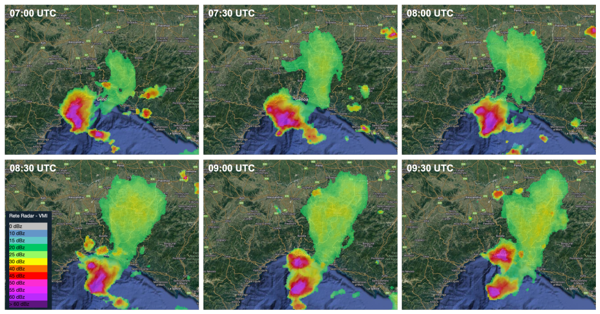
On the 14 August 2018 early in the morning (07:00 UTC, 09:00 local time) a deep convective thunderstorm developed in the Ligurian Sea, approximately 50 km to the southwest of the city of Genoa. The thunderstorm moved eastward over the sea and split into two cells. The cell to the north impacted Genoa approximately at 09:00 UTC. Figure 1 shows the evolution in space and time of the cell(s) through the Vertical Maximum Intensity (VMI) of the radar reflectivity measured by the meteorological Doppler radar of the Liguria Region. VMI values are always above 50 dBZ and the cloud top height (shown in Burlando et al. [36]) estimated from the Meteosat Second Generation (MSG) satellite measurements was above 12,000 m when the cumulonimbus cloud approached the city from the southeast.

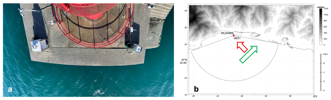
In the western entrance of the port of Genoa (at geographical coordinates 8.776764° E and 44.417497° N, referred to the WGS84), at the tip of the inner breakwater pier, at 5 m Above the Sea Level (ASL), near the all-round red light signal that is mounted on a light tower to mark the entrance, the Giovanni Solari Wind Engineering and Structural Dynamics (GS-Windyn) Research Group of the University of Genoa installed in April 2018 a Windcube scanning LiDAR WLS400S (funded by the European Project THUNDERR [37]). Just a few meters apart in the same place (Figure 2a), the Port Authority had installed a Windcube V2 vertical profiler in 2015 (funded by the European Project “Wind, Ports and Sea” [38,39]). Both instruments were operational when the thunderstorm approached Genoa and measured a downburst that hit the western part of the city. During this event, the storm motion was on average about 5 m/s from the southwest and when the downburst developed, the cloud was a few kilometers off the coast, so the main thunderstorm outflow recorded by the instruments was approximately from the southeast, which is orthogonal with respect to the storm motion (Figure 2b).

The Windcube V2, called hereafter GE51, measures the 3 components of the wind, $(u,v,w)$ (which are respectively the zonal west-to-east component, the meridional south-to-north component, and the vertical component), simultaneously at 12 heights Above Ground Level (AGL), namely 40, 50, 60, 80, 90, 100, 120, 140, 160, 180, 200, 250 m, with a sampling rate equal to 1 Hz. Accordingly, GE51 measures vertical wind profiles only within the surface boundary layer, where the well-known nose-like shape profile is often detectable during downbursts. GE51 is not expected, however, to measure the whole vortex ring produced by downbursts (e.g., the Primary Vortex, PV), whose height is typically on the order of a few hundred meters [40]. More details concerning how GE51 works and some examples of thunderstorm outflow measurements can be found in Canepa et al. [41]. The scanning LiDAR, called hereafter WLS400S, was configured to work in PPI (Plan Position Indicator) mode along 4 subsequent scanning paths covering the azimuth from 100° to 250° with 1.5° resolution (100 lines of sight) and 4 different elevations, 2.5°, 5.0°, 7.5°, 10.0°. An entire cycle of 4 scanning paths is completed in slightly less than 4 min (approximately 1 min per scan). WLS400S measures the wind component along the line-of-sight (i.e., the radial wind component), $v_l$, from 300 m to almost 14,000 m with a resolution of 88 m, which corresponds to 159 measures per line-of-sight.

Data measured by both instruments are temporally correct because they have a clock synchronized with a NTP server, while they are spatially correct because they were aligned with respect to geographic north during their installation. A sampling rate of 1 Hz allows the evolution of the phenomenon to be properly observed, as thunderstorm develops within 20–30 min. In terms of uncertainty, the accuracy of the scanning LiDAR radial wind speed is better than 0.3 m/s, while the accuracy of the vertical profiler is 0.1 m/s on wind speed and 2° on wind direction.

3. Numerical Model Configuration

The CM1 cloud model [42] version release 21.0 is used in Large-Eddy Simulation (LES) configuration to perform simulations of the thunderstorm described in Section 2. The governing equations that CM1 uses conserve mass and total energy, even though they might not be fully conserved in the model due to limitations in numerical integration. We chose the default LES configurations available also to avoid specific physics, forcings, or configurations as those related to the Planetary Boundary Layer (PBL) conditions or to particular weather phenomena. Time stepping to numerically solve the equations is performed with the Runge-Kutta 3rd order scheme, while the Klemp-Wilhelmson time-splitting method for acoustic modes is used for the pressure solver, with explicit calculations of acoustic terms in both vertical and horizontal directions. The advection terms are discretized using a fifth-order spatial discretization for both scalars and velocities, selecting this default option in the namelist as it does not require additional artificial diffusion. The Morrison’s double-moment scheme [43] is used for microphysics. Two simulations have been carried out using different subgrid-scale turbulence models: the first case, called CM1-TKE hereafter, applies a subgrid turbulence kinetic energy (TKE) prediction scheme and subgrid-TKE is then used to determine the eddy coefficients of viscosity and diffusivity, according to Deardorff [44]; the second case, called CM1-Smag, is based on a Smagorinsky model that assumes steady and homogeneous subgrid turbulence [45]. Terrain-following coordinates to map the model levels to the terrain are adopted, with the model top at a constant height.

Table 1. Namelist options chosen for the simulations.

Namelist Option	Choice
Numerical approach	Large Eddy Simulation
Subgrid turbulence	Deardorff’s [44] and Smagorinsky’s [45] scheme
Microphysics	Morrison’s [43] scheme
Lateral boundary conditions	Open radiative
Top boundary condition for wind	Free slip
Bottom boundary condition for wind	Semi-slip
Surface conditions	Temperature (land and sea) and moisture fixed over time

provides further details on the model’s boundary conditions adopted.

3.1. Model Grid and Input Data

The computational domain is squared, 289 km × 289 km × 20.3 km in the x, y, and z directions, respectively. A stretching factor is applied along the horizontal, with spacing varying from 50 m in the innermost part of the domain to 1.8 km at the external boundaries. The stretching factor (i.e., the ratio between subsequent horizontal space steps) is constant and equal to 1.012. The total number of grid points is 600 × 600 in the x and y directions. The horizontal grid has been stretched in order to have a higher resolution in the centre of the domain, where the storm is supposed to develop, intensify and interact with the complex orography of the Ligurian region, as well as to save computational time by reducing the resolution outside the storm. The stretching factor is chosen to make the resolution change smoothly in order to avoid any kind of numerical discontinuity and instability. Along the vertical, the grid resolution is 25 m from the ground up to an altitude of 500 m and 200 m from 2.3 km to the top of the atmosphere assumed at 20 km (i.e., within the stratosphere). In between (i.e., from 500 m to 2.3 km) the grid is stretched using an internal CM1’s procedure. The total number of vertical levels is 126. Such a fine grid along the vertical in the first kilometers from the ground has been chosen to better resolve and explicitly describe the processes that occur within the ABL and the downburst itself.

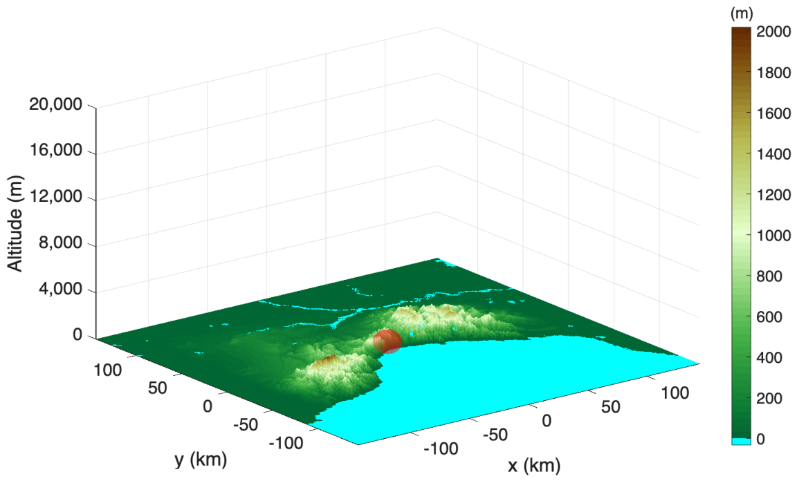
In the simulations, surface heat and moisture fluxes and other surface properties, as well as a detailed orography, are included. As far as the description of the surface properties is concerned, we used the ERA5 (ECMWF Reanalysis v5) reanalyses for the land surface temperature and deep-layer temperature of the soil, with resolution 0.25° × 0.25°, the USGS land cover data for land cover classification, and satellite observations available from the Copernicus Marine Service dataset for the SST, both at a resolution of 0.01° × 0.01°. The orography has been downloaded from the SRTM database, with an original horizontal spatial resolution of 90 m. As the orography in the computational domain is very steep at the external boundaries, it has been smoothed applying a cosine function within a buffer frame of a few kilometers from the boundaries to avoid numerical instabilities. Finally, surface and orography data have been interpolated from their native grids onto the computational grid using a cubic spline interpolation. Figure 3 shows the orography after smoothing it at the boundaries and interpolation.

3.2. Thunderstorm Initiation

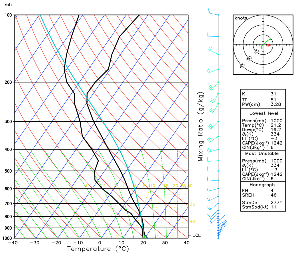
In CM1 the vertical tropospheric conditions have been assumed to be horizontally homogeneous within the whole computational domain. Accordingly, these atmospheric conditions have been retrieved from the ERA5 profiles of wind, temperature and dew point temperature (i.e., humidity) corresponding to 07:00 UTC in a grid point offshore the city of Savona (Lon 8.5° E, Lat 44.25° N), where the thunderstorm initiated in the morning before splitting into two cells (see Section 2). These initial conditions are reported in Figure 4, which shows the corresponding radiosounding data.

It can be seen that just before the event the air column appears unstable and the Convective Available Potential Energy (CAPE) is well vertically distributed and up to a significant value of more than 1200 J/Kg⁻¹, with a moist atmosphere at the lowest levels, making the Lifting Condensation Level (LCL) very close to the surface, around 970 hPa. The convective inhibition (CIN) is almost negligible, and the K-index [46], one of the main stability indices used to determine the probability of thunderstorm occurrence, has a value for the area of interest equal to 31 °C, which falls within the range associated with moderate thunderstorm potential [47]. Such conditions are the required ingredients for deep convection formation in conjunction with the outbreak of a front, which acts as a lifting mechanism. This is indeed the most probable forcing mechanism that made the air parcel rising to the level of free convection and led to the thunderstorm development, considering that on 14 August in the morning colder winds were blowing from the north (confirmed by full-scale measurements [36], see also Figure 5 until 09:00 UTC) along the coast between Savona and Genoa, while southerly warmer winds were blowing over the sea.

Since CM1 does not allow to initiate the storm trough frontal wedging, as the model requires the same initial conditions everywhere taken from a single radiosounding for the whole domain, the storm was generated by using the warm bubble technique [30], as done by [22]. Accordingly, a 3D bubble located at 1 km ASL, with a horizontal and vertical radius of, respectively, 10 km and 1 km, was set in the Ligurian Sea, southwestward of Genoa (Figure 3). The bubble positioning was chosen via trial and error until the resultant thunderstorm was approximately centered in the position that it had at 09:00 UTC according to radar data (see Figure 1 and Figure 2b). The positive anomaly in potential temperature for the warm bubble was adjusted to +3 K to ensure that the corresponding surface wind velocities of the downburst closely matched the measured values. This also falls within the range of values typically used in works which use CM1 to initialized severe convection bringing to Mesoscale Convective Systems (MCS) and supercells [48,49,50].

Both simulations run for a period of 90 min after the warm bubble is released into the atmosphere. Outputs are saved every 5 min in the first 30 min, when the thunderstorm is in the initial stages until the updraft has reached the maximum altitude, and every 30 s in the last 60 min. This choice allows analyzing in great detail the time/space evolution of the thunderstorm from the downdraft formation to the downburst dissipation at the ground.

3.3. Details on the Computing Resources

High-computing resources from GALILEO100 calculator of the Italian Northeastern Inter-University Consortium for Automatic Computing (CINECA) have been used to run all the simulations. The system architecture consists of 636 computing nodes each 2 × CPU Intel CascadeLake 8260, with 2.4 GHz, 384 GB RAM, subdivided in different partitions. For the scopes of this work, the partition composed of fat nodes (memory per node 3 TB) has been chosen, with the usage of 24 nodes and 25 processor cores per node for each simulation. The time required to run each case depends on both the microphysics and the turbulence schemes adopted, due to different cloud compositions and thunderstorm evolutions, ranging between 3 and 11 h.

4. Validation of the Thunderstorm Simulations

The present section reports the validation of CM1’s simulations using observations from both the LiDAR systems described in Section 2.

4.1. Comparison with the Measurements of the LiDAR Vertical Profiler

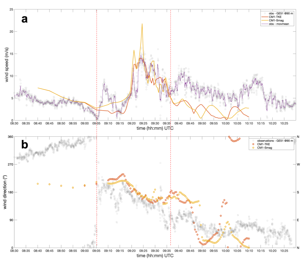
Before CM1 simulations are compared with anemometric LiDAR measurements, the signals have to be properly synchronized. This is needed because CM1, as opposed to the meteorological models that use the UTC time frame, does not refer to an absolute time-reference system. Accordingly, simulation time steps, which are relative times, have to be assigned the corresponding values in UTC. This is done aligning the signals of simulated and measured wind speed (horizontal components only) at a reference position that is chosen to be the location of GE51 at 90 m AGL. This height is chosen because it is neither too close to the ground (minimum measurement height is 40 m AGL), hence avoiding possible very local effects on the flow due to the presence of the pier and the red light signal that cannot be taken into account into simulations, nor close to the top measurements (maximum measurement height is 250 m AGL) whose signals usually have a larger number of undefined values. In addition, this is the height where the maximum of the nose-like shape profile of the downburst is recorded. The alignment is based on the calculation of the correlation coefficient, $\rho$, in between 09:05 UTC and 09:37 UTC: CM1 signals are shifted until the maximum $\rho$ value within this time range is obtained. The time range for correlation mentioned above is chosen in order to focus on those parts of the signals that correspond to the downburst occurrence only. This is done because CM1 does not simulate the real weather conditions before and after the downburst, which makes useless and meaningless the comparison of signals outside the downburst time limits. According to this procedure, the initial time step of CM1 was set at 08:40 UTC.

Figure 5 shows the comparison between the time series of wind speed and direction measured and simulated at the reference position (i.e., GE51 at 90 m AGL), after signals are properly aligned. Figure 5b, in particular, can be useful to identify the selected period of occurrence of the downburst, which is between 09:05 UTC and 09:37 UTC. Before 09:05 UTC, the wind was from the northeast with wind speed around 5 m/s, which is coherent with the radiosounding of re-analyses reported in Figure 4 that shows light winds blowing from NE in the first 1000 m ASL (between 1000 and 900 hPa). The weak north-easterly winds at the surface are due to a local effect along the coastline, influenced by the complex orography. This typically occurs when an Atlantic trough or front approaches the Ligurian Sea from the west. Replicating the exact mesoscale conditions in CM1 is challenging, as the model requires a single atmospheric sounding for the entire computational domain. This is ideal for idealized simulations but unsuitable for simulating the full evolution of the storm. Therefore, by choosing the warm bubble technique to trigger the storm and simplifying the sounding, the focus is only on the north-eastward forcing aloft to correctly set the storm’s motion. At 09:05 UTC the wind direction suddenly changes, marking the onset of the thunderstorm outflows blowing from the downdraft touchdown position, shown in Figure 10a (red circle). From 09:05 to 09:37 UTC, the wind direction keeps on backing, following the thunderstorm track until it blows from the first quadrant (0°–90°). At this point the wind direction cannot be related to the thunderstorm anymore because wind blows from a direction that is almost opposite with respect to the touchdown position. As far as the wind speed is concerned, in the same period two distinct phases can be distinguished: between 09:05 and 09:15 UTC an isolated peak that might be related to some gust front preceding the stronger downburst, occurs; between 09:15 and 09:37 UTC the main downburst is recorded. In the latter period, the wind speed is not particularly high in absolute terms: the maximum gust is 16.4 m/s and the maximum value of the moving mean wind speed (purple line in Figure 5a), averaged over $T=30$ s according to Zhang et al. [51], is 14.8 m/s.

Overall the simulations follow the same trends of the observed wind speed and direction within the period 09:05–09:37 UTC. The main difference is that CM1 does not simulate the gust front between 09:05 and 09:15 UTC. The observed peak could have been due to a localized mesoscale feature, such as a weaker outflow boundary of a pre-existing thunderstorm cloud. Investigating the physical drivers behind this early gust front (09:05–09:15 UTC) would be crucial to understand why it was not reproduced by the CM1 model. Unfortunately meteorological observations needed to understand precisely, beyond any reasonable doubt, what this peak was and what it was really due to is not available. However, as a matter of fact (see Figure 1 and the thunderstorm evolution described in Section 2), the initial cloud genesis was well before, in time and space (around 7.00 UTC in Savona), with respect to the thunderstorm landing in Genoa, which in its turn is actually derived from the northern cell after the system born in Savona separates in two independent systems during a process of symmetrci split (see Figure 1 at 9.00 UTC). Following these considerations, the whole system (and both the northern and southern splits) is thought to be a multicellular system, with multiple cells developing as the system approaches Genoa. In this study, CM1 is not simulating the whole evolution of the multicell system, but only the single cell that landed in Genoa. According to the analysis performed in Section 4, the simulated cumulonimbus cloud can be considered a good replica of this particular cell, while all the phenomena that are related to pre-existing cells (e.g., the outflow boundary mentioned above) are not simulated.

However, both the ramp-up phase of the downburst (between 09:15 and 09:21 UTC in Figure 5a) and the dissipation after the highest peak (between 09:25 and 09:37 UTC in Figure 5a) are properly captured in terms of trends as well as intensity. CM1-Smag shows 3 distinct peaks at about 09:21, 09:25, and 09:28 UTC that are present in the observations as well, even if the first two peaks are overestimated by the model. CM1-TKE shows overall a smoother behavior with respect to both CM1-Smag and observations. Some metrics are reported in

Table 2. Comparison between observations and simulations. Metrics calculated in the time range between 09:05 and 09:37 UTC.

Metric	CM1-TKE	CM1-Smag
$\rho$ (-)	0.82	0.79
U ME (m/s)	−0.23	0.95
U RMSE (m/s)	2.42	2.72
$\theta$ ME (deg)	36.6	34.7
$\theta$ RMSE (deg)	47.0	42.8

to quantify the performance of CM1. The correlation coefficient $\rho$ calculated using wind speed is around 0.8 for both simulations. $\rho$, as well as the other metrics based on wind speed, is penalized by the gust front between 09:05 and 09:15 UTC that is not simulated by CM1. The mean error, ME, for wind speed U is very close to 0 for CM1-TKE, whereas it is almost 1 m/s for CM1-Smag, which overestimates the observations in the first two peaks at 09:21 and 09:25 UTC. The root mean square error, RMSE, for wind speed is around 2.5 m/s for both simulations. As far as the wind direction $\theta$ is concerned, ME and RMSE values are similar for both CM1-TKE and CM1-Smag, around 30° and 45°, respectively. In general, MEs and RMSEs are in line with the typical values found for meteorological models [52] and re-analyses [53], when compared to synoptic winds.

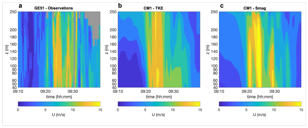
In addition to the time series compared above, the evolution in time of the wind speed for the entire vertical profiles is reported in Figure 6 for GE51 observations (a), CM1-TKE (b), and CM1-Smag (c). All figures show measurements or simulations taken from 09:10 to 09:40 UTC. During this period, which corresponds to the downburst occurrence, the 3 peaks already noticed in the GE51 observations and CM1-Smag simulations (Figure 5a) at 09:21, 09:25, and 09:28 UTC are also well distinguishable. In particular, all the 3 peaks correspond to periods during which the vertical profile assumes the well-known nose-like shape. The first measured peak is shorter and weaker. The second and third peaks are longer-lasting and stronger. Although CM1-Smag produces higher wind speed values with respect to the observations, it is able to replicate all the 3 peaks (i.e., nose-shape profiles) surprisingly well in terms of timing, durations, and vertical extension. CM1-TKE, on the other hand, replicates the 3 peaks with lower accuracy: overall this simulation provides a flatter temporal trend of downburst wind intensity, since the first and second peaks are not well separated, and the third peak is very weak and short compared to observations.

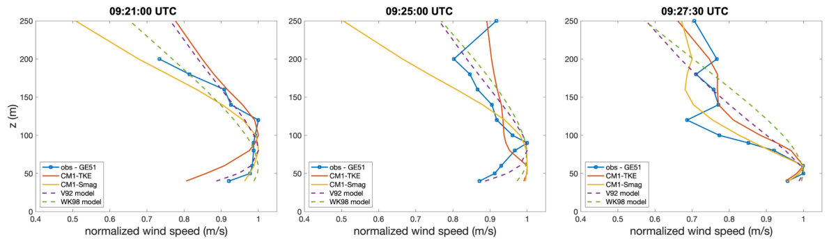
Vertical wind profiles simulated by CM1 during the identified peak times are evaluated against observational data and two established analytical downburst models (Figure 7): the Oseguera-Bowles-Vicroy model [54,55,56] (called hereafter V92) and the Wood and Kwok model [57,58] (called hereafter WK98). All profiles are normalised by their respective maximum wind speed to facilitate intercomparison. At 09:21:00 UTC, both CM1-Smag and V92 accurately reproduce the characteristic nose-shaped structure evident in the observed profile. However, V92 exhibits notable divergence from the observational data above 160 m AGL. In contrast, WK98—and to a greater extent, CM1-TKE—deviate more substantially from the measured profile throughout the column. At 09:25:00 UTC, V92 demonstrates the highest fidelity in replicating the observed wind structure. WK98 and CM1-Smag exhibit comparable behavior near the surface, though both slightly overestimate wind speeds. CM1-TKE, by contrast, yields an anomalously uniform profile above 80 m AGL, with a modest acceleration near the surface. By 09:27:30 UTC, observational data indicate a downward shift of the nose-shaped maximum toward the surface, with wind speeds remaining nearly constant above 100 m AGL. Under these conditions, neither V92 nor WK98 adequately captures the observed profile. Conversely, both CM1-TKE and CM1-Smag exhibit good agreement with the vertical wind structure, effectively replicating the measured evolution.

4.2. Comparison with the Measurements of the Scanning LiDAR

Each scan of the LiDAR WLS400S refers to a time period of about 50 s, which is the time required by the scanning head to move from the azimuth 100° to 250°. Accordingly, the scans are not really instantaneous wind fields. The outputs of the CM1 simulations are saved precisely every 30 s, instead (in the time range of downburst occurrence), hence the corresponding wind fields are really Eulerian representations of the flow conditions. For comparison purposes, we interpolated the simulated wind fields over the same PPI scanning paths (i.e., azimuth from 100° to 250°; zenith angles 2.5°, 5.0°, 7.5°, and 10°; 100 lines of sight, one every 1.5° azimuth; 159 gates per line of sight with resolution 88 m from 300 m to ∼14,000 m) of the WLS400S. Arguing that 50 s is a time short enough to consider the observed wind fields frozen (i.e., under the Taylor hypothesis for large eddies), one could compare the measured scans with the simulated wind fields corresponding to the time step closer to the initial recording time of the scanning path (i.e., the line of sight at 100° azimuth). However, we decided to perform also a linear time interpolation among the simulation outputs in order to properly take into account the evolution of the simulated wind fields. For instance, instead of comparing the WLS400S scan taken at 9:18:31–9:19:21 UTC with the simulated scan at 9:18:30 UTC, each simulated line of sight is calculated through a linear time interpolation between the simulated scan at 9:18:30 and the following ones (i.e., at 9:19:00 and 9:19:30) based on the timestamps of the measured line of sights.

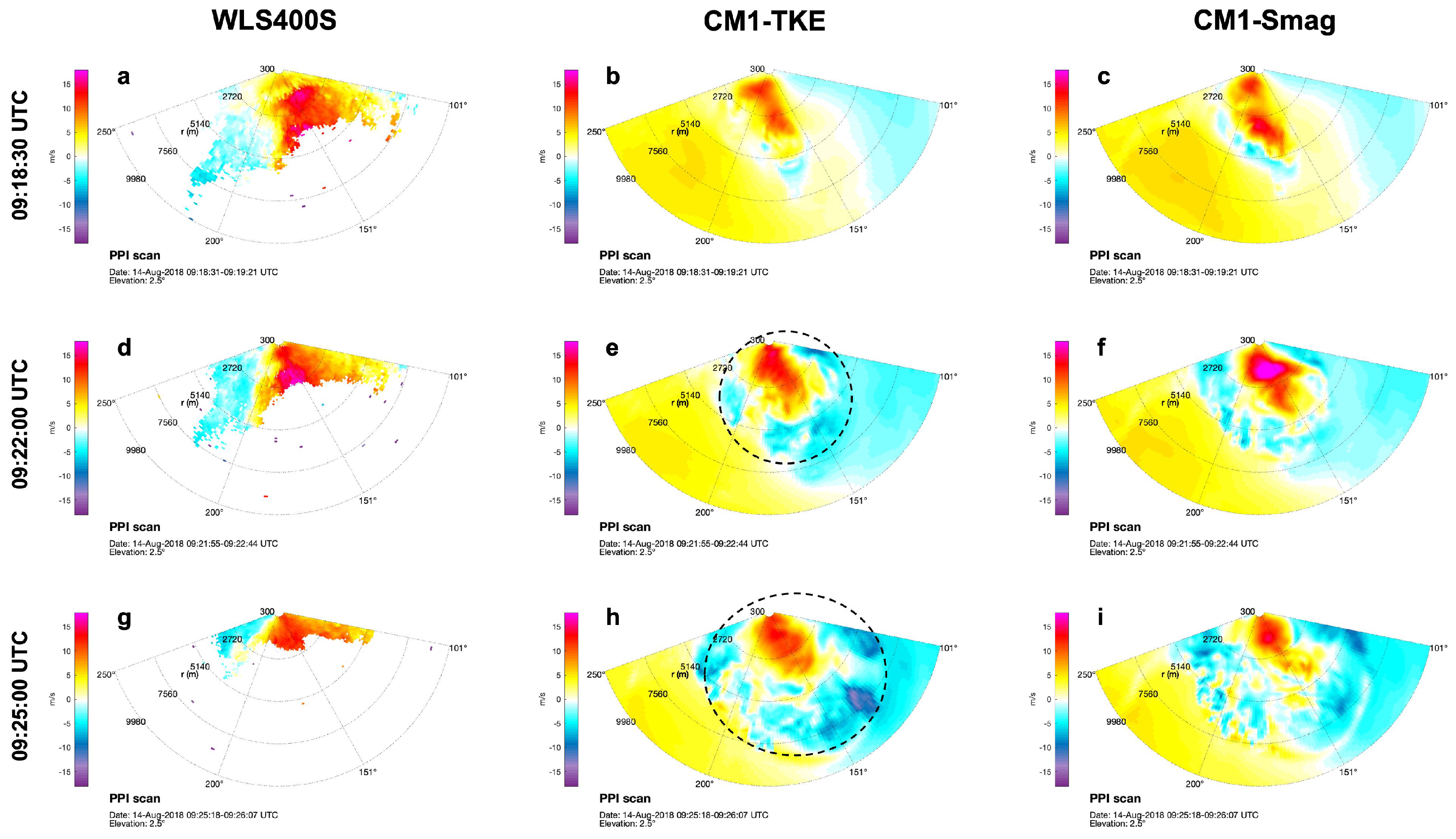
Figure 8 shows the spatial distribution of the radial wind velocity component measured by WLS400S and simulated by CM1 at 3 different times. All PPIs correspond to the zenith angle equal to 2.5°, which is chosen because it is the most similar to the horizontal winds. Moreover, PPIs are cropped at ∼10 km from the instrument, to better focus on the downburst. At 09:18:30 UTC, the downburst is approaching the instrument (Figure 8a) with its Primary Vortex (PV) ring, according to the circular shape of the gust front that, a couple of km from the instrument, has already reached more than 15 m/s. From the time series point of view, this is the so-called ramp-up phase (see Figure 5a) that precedes and lasts until the PV reaches the instrument. In both the CM1 simulations (Figure 8b,c), the development of the PV is slightly delayed and the PV has not reached yet at this time the observed intensification level. Moreover, the main approaching direction simulated is here slightly shifted (∼20°–30°) from the observed one (see Figure 5b). Part of the measured PPI scan (Figure 8a) is missing due to the heavy rain that follows the gust front of the PV. The same area is however available from simulations, showing a light negative region (∼−5 m/s) at a bit more than 5 km from the center at azimuth angles around SSE. This area corresponds to the rear side of the PV. It is rather clear from the simulated patterns that the touchdown position was about 5 km at 170°. Finally, it is worth noting that the light blue area southwest of the downburst is instead yellow in CM1 simulations. Again, this is due to the fact that CM1 was initialized with southwesterly winds all within the troposphere to properly simulate the storm motion, while in reality near the coastline in the lower part of the troposphere the wind was blowing from the northern quadrants. This is, however, a local effect that could not be replicated in CM1 and that did not affect the thunderstorm formation and evolution that much.

At 09:22:00 UTC, the PV reaches the instrument. This is the first peak recorded by GE51 (see Figure 5a). At this time, both CM1 simulations have developed a strong PV, whose intensity is comparable to the observed one. The shape and extension of the PV are similar between simulations and observations. Yet, CM1-Smag overestimates the observations and the maximum radial wind speed is about 22 m/s in the magenta area 2 km SSE from the center. At 09:25:00 UTC, another gust front reaches the instrument. This can be recognized as the second peak in Figure 5a, which is also the strongest one. In addition, from CM1 simulations one can observe the overall extension of the downburst, which is marked by the blue areas of negative radial wind speed all around the positive maximum (see circles in Figure 8e,h). From 09:22 to 09:25 UTC the downburst increases its diameter from about 5 km to 8 km in CM1-TKE.

5. Discussion

In the following Section 5.1, the thunderstorm simulated by CM1 using the Smagorinsky scheme for turbulence, i.e., CM1-Smag, is first described with emphasis on the updraft, downdraft, and downburst formation and evolution in time. For the sake of simplicity, CM1-Smag is only shown here because CM1-TKE is rather similar from the point of view of the general and macroscopic characteristics of the thunderstorm. The cloud evolution in cumulus, mature, and dissipation stage, is also comparable between CM1-Smag and CM1-TKE. The main difference between these simulations is the very local structure of the flow fields, as shown in Section 4.

5.1. Morphology and Evolution of Updraft and Downdraft

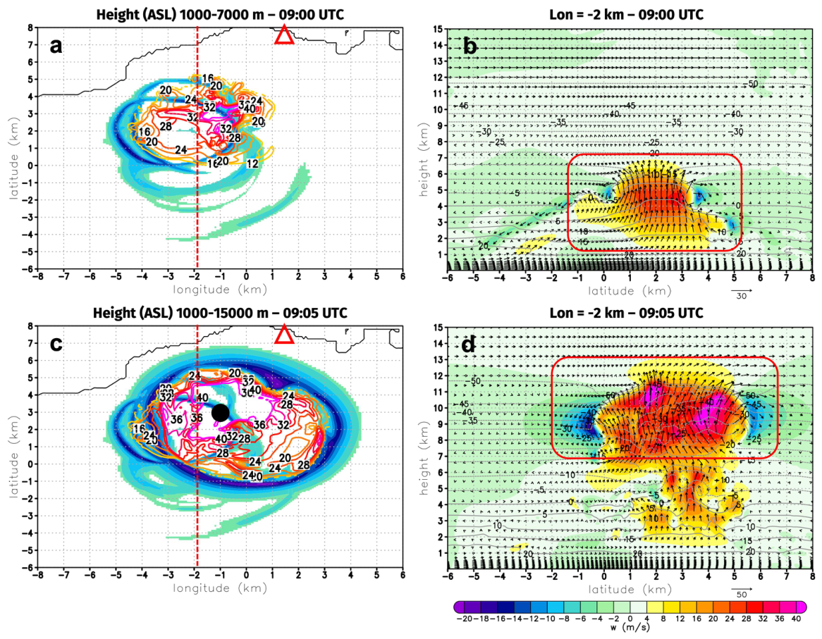
In the CM1 simulations, the warm bubble starts developing the updraft around 08:55 UTC (for time referencing refer to Section 4.1) and in about 10 min the updraft reaches the top of the troposphere. The maps on the left in Figure 9 show the horizontal development and extension of the updraft through the maximum w values in the troposphere at 09:00 UTC (Figure 9a) and at 09:05 UTC (Figure 9c). The vertical sections on the right (Figure 9b,d) show at the same times the cross-sections at longitude −2 km. According to Figure 9b, at 09:00 UTC the updraft (red box) had already reached almost 7 km ASL in altitude and the maximum vertical wind component w was in the order of 30 m/s. Five minutes later, at 09:05 UTC (Figure 9d), the updraft reaches the top of the troposphere at 12 km ASL and the maximum vertical velocities are higher than 40 m/s in the upper part of the cloud, bringing about an overshooting that reached approximately 13 km ASL. Comparable high values of the updraft are reported in the literature, for instance by Wienhoff et al. [59] in their Figure 12, who estimated $w>35$ m/s for the vertical wind field obtained from dual-Doppler radars at 3.5 km in a tornadic supercell. While the updraft grows, a 1–2 km deep vortex ring develops all around the core of positive w values. The size and shape of the ring can be seen in Figure 9a,c by the rounded dark blue ($w<-10$ m/s) shaded contours, which are minimum values along the tropospheric column: Figure 9a refers to the layer between 1 and 7 km ASL during the first development of the updraft; in Figure 9c the larger vortex ring superimposed to the ones present in Figure 9a corresponds to the upper part of the cloud, with an overall extension of about 8 km in diameter. It is worth noting that the updraft also translates eastward while uplifting due to the atmospheric westerly flows that were blowing on 14 August in the morning (see Figure 4).

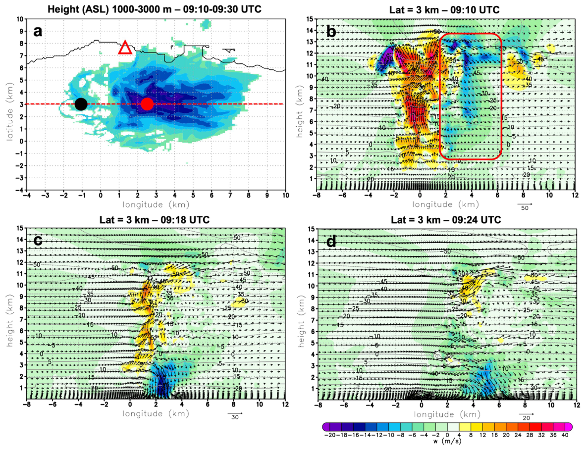
After the updraft has reached the top of the troposphere, a deep downdraft is initiated on the lee side (eastern) of the anvil cloud. Figure 10 shows the development of the downdraft from the top of the troposphere to the ground and its dissipation, which overall occurs in approximately 15–20 min. In particular, Figure 10a shows the location of the downdraft in the lower 3 km ASL, where it is stronger and therefore more easily detectable. The red circle, which is approximately in the center of the maximum downdraft (i.e., the minimum vertical velocity component) shows that it occurs at about 3.5 km eastward with respect to the position of the maximum updraft center (black circle). If we assume that the downburst spreads out at the ground more or less radially from the red circle, the direction of the thunderstorm outflows measured at the LiDAR location should be from the south-southeast.

In Figure 10b–d, the wind vectors of the ($u,w$) components and w (shaded contours) along the cross section taken at latitude 3 km (red dashed line in Figure 10a) are reported. Figure 10b shows that, about 5 min after the updraft overshooting (09:05 UTC), the downdraft is already well developed and has reached almost 3 km ASL. Except at the very top of the downdraft where w is somewhere around −15 m/s or lower, vertical wind velocities are around −10 m/s in between 3 and 10 km, which is not very high and much lower than the updraft. However, upon reaching about 3 km ASL, the downdraft starts accelerating (Figure 10c) more likely due to hydrometeor frictional drag that makes the downdraft more negatively buoyant. The process continues until touchdown, which occurs precisely at 09:18 UTC. Afterwards, a downburst develops at the ground with multiple vortex rings (see next section) and the cloud starts slowly dissipating.

5.2. Downburst Development and Characteristics

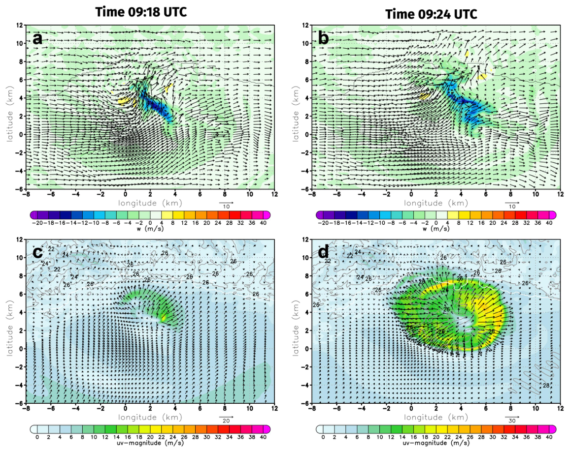
The downdraft in the lowest part of the troposphere during the thunderstorm mature stage seems to be wide about 2–3 km, according to Figure 10c that refers to 09:18 UTC, while the downburst diameter appears to be wide about 6 km. Following the classification proposed by Fujita [60], the latter size corresponds to a macroburst (i.e., size > 4 km). However, the shape of the downdraft in this thunderstorm is neither regular nor steady. In CS as well as IJ models, the downdraft is usually assumed to have a rounded (spherical, elliptical, or cylindrical) shape, which forces the downburst to be axisymmetric at the ground. CS models are known to provide a more realistic dynamical forcing of downbursts and replicability of some of their thermodynamically driven properties, such as baroclinically generated vorticity in the outflow [61]. However, the low outflow velocities involved in this typology of experiments lead to favor the IJ approach. On the other hand, the latter approach suffers from the stationarity of the outflow after the passage of the primary vortex and cannot capture the buoyancy-driven nature of the phenomenon, thus partially missing the full physical representation of it [61,62]. An aspect highlighted in some papers [63,64,65] and related to the IJ approach is the lack of a clear distinction between the translational movement of the thunderstorm cell and the boundary layer wind in which the thunderstorm outflow is immersed at the ground. In full cloud simulations initiated by a warm bubble, the initial regular shape of the bubble is soon lost and the downdraft is free to develop an irregular and complex shape. This is the case in the present simulations, where the downdraft during the mature stage of the thunderstorm is more similar to a blade. Figure 11a shows how the downdraft (shaded contours) looks like at 09:18 UTC in a horizontal section taken at 1000 m ASL: the blade-shape of the downdraft is oriented along the direction NW-SE and is more than 5 km in length. At the same time, the downburst has just started developing at the ground, as shown in Figure 11c, with horizontal wind speeds as high as 10–15 m/s ahead of the storm. At 09:24 UTC, the downdraft assumes an irregular shape (Figure 11b), while the downburst at the ground reaches its maximum speed of around 25 m/s in the same direction as the storm motion. This is rather interesting as it seems to suggest where the highest velocities in the downburst can be found given that the storm motion is known, which is often the case when observations from a meteorological radar are available. Moreover, despite the irregular shape of the downdraft, the downburst still develops to a good extent axisymmetrically while spreading outward (Figure 11c,d). This seems to confirm that CS and IJ models can replicate real downbursts even though they adopt regular shapes of the downdraft.

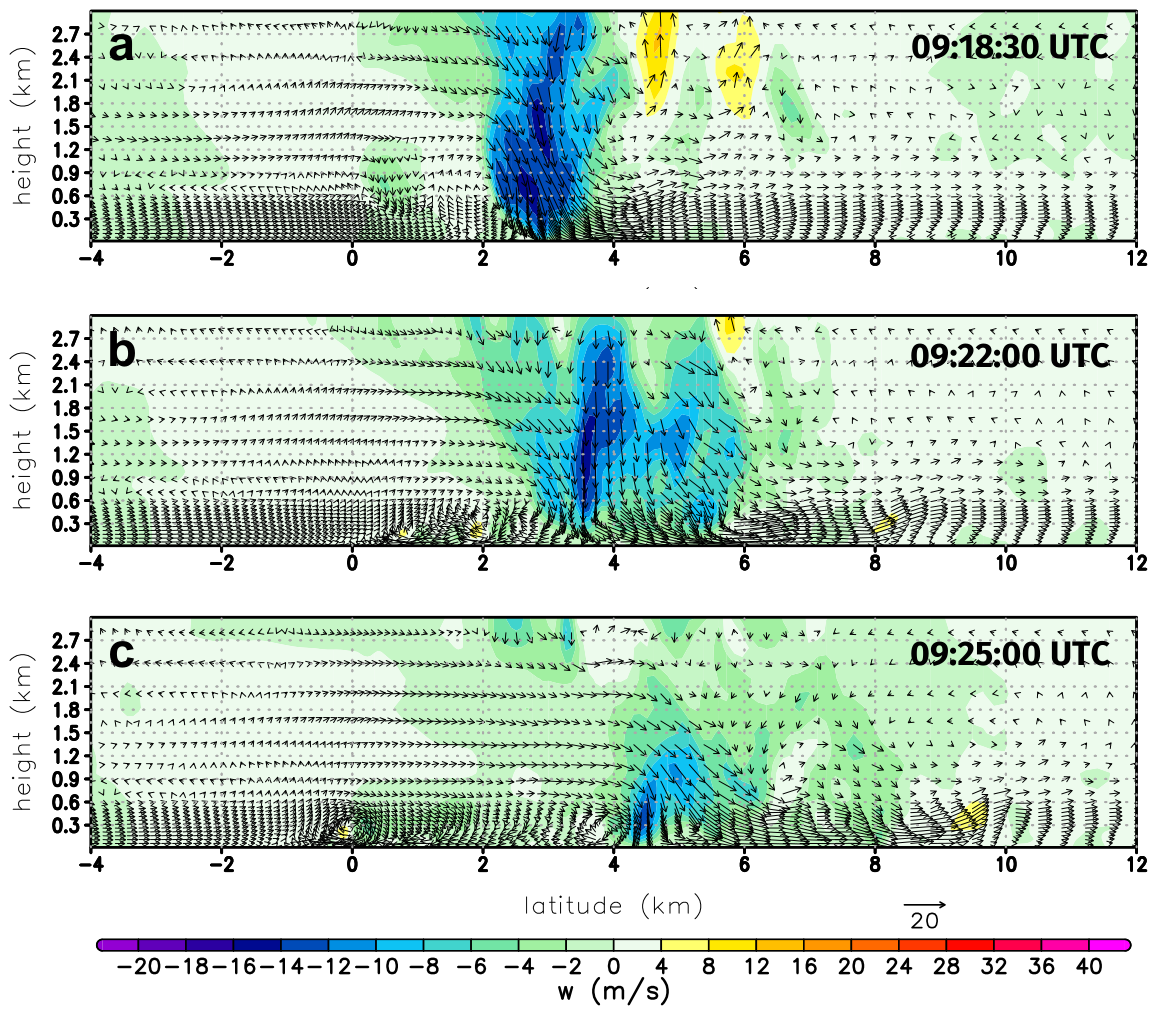
The analysis of the downburst produced at the ground reveals some interesting features, which are shown in Figure 12. This figure presents some vertical sections taken at Longitude 3 km, which corresponds approximately to the center of the downdraft in Figure 11, at 09:18:30 (Figure 12a), 09:22:00 (Figure 12b), and 09:25:00 UTC (Figure 12c). These times are the same as reported in Figure 8, allowing a direct comparison between the two figures. In Figure 12 the vertical velocity component, w, is shown in shaded contours, whereas vectors correspond to the $vw$-components and their intensity is shown through the arrow scale in the bottom right. At 09:18:30 UTC, the downdraft touches down and the downburst starts developing at the ground. It is worth noting, however, that two downdrafts occur at the same time, a secondary one rather weak (i.e., w about −5 m/s) at a latitude of about 1 km, the main one at a latitude of about 3 km with vertical velocities larger than 20 m/s. Moreover, inside the main downdraft, several gusts (i.e., dark blue areas) can be seen that will produce pulsating impingements at the ground which, in turn, will bring about multiple vortex rings or gust fronts. These pulses, in agreement with Fujita and Wakimoto [66] and based on the scales that the model can reproduce, should be classified as microbursts embedded within the larger downburst. The result is also in agreement with the main finding of [22]: their analysis reveals a very complex evolution dominated by rapidly fluctuating winds and complex precipitation patterns driving highly variable local downdrafts embedded within the main downbursts that are spawned by the simulated thunderstorm.

2.5 min later, at 09:22:00 UTC (Figure 12b), a couple of vertical gusts within the main downdraft have reached the ground and produced two distinct vortex rings. However, the vortex rings look very different on the southern and northern sides of the developing downburst. On the southern side, two vortices about 0.5 km deep can be found at latitude 1 and 2 km. On the northern side, there are no clear vortices but nose-shape profiles from 4 to 8 km, with variable heights of the maximum horizontal velocity. Noteworthy, around latitude 5.5 km the height of the nose is very close to the ground due to an overlaying vertical gust that squeezes the nose-shaped profile below. In addition, between 8 and 10 km a reversed flow due to the boundary layer detachment can be seen that displaces the nose-shape profile upwards. This asymmetry between the southern and northern sides is due to the interaction between the downdraft, which is translating with the parent storm towards NE, and the ABL flow that blows from the SW in the simulations. On the southern side, the vortex rings propagate in the opposite direction of the ABL, but the vorticity has the same sign for both flows. This favours the entrainment of the ABL into the vortex rings and contributes to making the vortices longer-lasting through the conservation of rotational flow. On the northern side, the ABL flow and the vortex rings have opposite circulations. This makes the vortex rings break down due to the unstable conditions induced by the opposing ABL wind.

At 09:25:00 UTC (Figure 12c), the downdraft is dissipating but a third vortex is now forming on the southern side, also forced by the entrainment of the ABL flow in the rear flank of the storm. The previous couple of vortices are still clearly detectable at 0 and 1 km of latitude, which means that their advection velocity was about 1 km in 3 min. On the northern side, the nose-shaped profile can be found until 10 km (a couple of km inland), while the boundary layer detachment has expired.

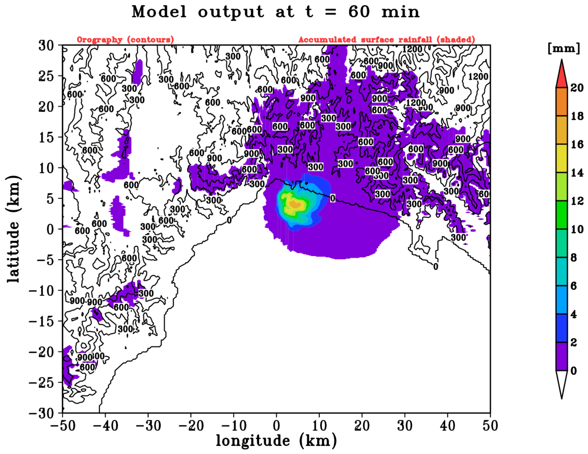
The accumulated precipitation simulated by the model at the end of the occurrence of the thunderstorm (during its dissipation phase at 09:40:00 UTC) is reported in Figure 13. By performing a broad comparison of Figure 11d with Figure 13, the highest precipitation values are located near the simulated highest wind gusts produced by the downburst. Lighter precipitations also appear to be more skewed towards the NE, thus in the direction towards which both the larger-scale flow and the downburst winds blow and produce more intense gusts. This characteristic seems to agree with the typical behavior of a wet downburst, whose precipitation distribution tends to strongly follow the direction and intensity of the most significant wind gusts.

6. Conclusions

The present paper focuses on simulating a downburst-producing thunderstorm that occurred in Genoa, Italy, on 14 August 2018, using the full cloud model CM1. This event is previously described from the meteorological point of view in Burlando et al. [36] and is now numerically simulated for three main purposes:

1.

To test several microphysics schemes for cloud model simulations and their performances in reproducing a real case study event and its main features.

2.

To demonstrate, through validating the simulated wind fields against LiDAR measurements, that full cloud models can realistically simulate the downbursts produced at the ground during thunderstorms.

3.

To enhance our understanding of the kinematic processes within the cumulonimbus cloud, specifically in terms of updraft and downdraft development.

4.

To provide the scientific community with the simulated wind fields in a public repository. The ultimate goal is to share a validated test case of a downburst, creating a benchmark accessible to scholars, researchers, and students in alignment with the Open Science principles.

Section 4 shows the comparison between the wind fields simulated at the ground during the downburst and the measurements from a LiDAR vertical profiler and a scanning LiDAR operated in PPI mode. Here the time series at a reference position over the vertical profiler are firstly compared and some standard indices (e.g., mean error and root mean square error for wind speed and direction) are calculated and used as metrics to evaluate quantitatively the performance of CM1. These metrics turned out to be comparable with the same metrics used to compare the wind field simulated using meteorological models during synoptic conditions. However, it is worth noting that thunderstorms produce rapidly evolving in time and spatially non-stationary wind fields that are much more difficult to be simulated with respect to synoptic conditions. This makes the results presented here particularly valuable, also considering that simulations are saved and compared every 30 s. Secondly, the comparison of the evolution of the vertical wind speed profiles up to 250 m AGL, which is the maximum height measured by the LiDAR, is shown in order to understand whether the modulation in time of the downburst simulated by CM1 resembles to some extent the observations. It was found that the simulation of CM1 carried out using a Smagorinsky scheme for turbulence is surprisingly similar to the observations in that it is able to replicate three peaks that were measured by the LiDAR with good timing and duration, even if the peaks are overestimated in this simulation. In Section 5.2, it is also shown that these peaks are due to subsequent vertical gusts within the downdraft that produce at the ground some pulsating impingements which, in turn, bring about multiple vortex rings or gust fronts that, spreading out from the touchdown position, are recorded as peaks by the LiDAR when they pass over the instrument. Thirdly, the PPI scans of the scanning LiDAR are compared with the concurrent outputs of the CM1 simulations. This analysis allows to understand how the overall structure of the downburst evolves in time and space, which is particularly useful because the signal of the scanning LiDAR is blind in those areas where heavy rain occurs, typically below the downdraft. According to the simulations, the size (i.e., diameter) of the downburst increases rapidly of about 1 km per minute.

After that the wind fields at the ground simulated using CM1 have been validated, in Section 5 the updraft and downdraft that developed within the cumulonimbus cloud are analysed. Here, it is assumed that they are at least plausible representations of the real ones, because unfortunately no direct measurements inside the cloud are available to understand to what extent the simulations are able to reproduce the entire thunderstorm. However, they are expected to be rather realistic considering that the simulated downburst is qualitatively and quantitatively similar to the observations. As a general consideration, it is shown that the structure of both updraft and downdraft is irregular and rather complex. While the updraft is forced to start from an elliptical warm bubble, it keeps this shape upon reaching the top of the troposphere, but within the bubble the field of positive vertical wind velocity is non-homogeneous, reaching in some regions 40 m/s. Interestingly, all around the bubble a counter-rotating vortex forms where negative vertical velocities can be as high as −20 m/s or more. The first downdraft seems to start from this vortex in the lee (with respect to the atmospheric flows blowing from SW) side of the thunderstorm and descends in a few minutes up to an altitude of 3 km ASL. Around this altitude, the downdraft associated with the downburst at the surface develops and, below 3 km, the flow accelerates to more than −20 m/s, most probably because of the hydrometeor frictional drag and producing a wet downburst at the surface. The downdraft that hits the ground has a shape similar to a blade, which becomes more and more irregular as the thunderstorm approaches its dissipation stage. Noteworthy, despite the shape of the downdraft is not regular as typically assumed in CS or IJ models (e.g., cylindrical), the downburst produced at the ground spreads out in a rounded shape that resembles the one produced in downburst-like impinging jets or downburst produced using a cooling source.

The choice of CM1 for our scopes has been strongly motivated by its being highly designated to simulate deep convective systems, due to its capability in providing high-resolved spatio-temporal details. The usage of this full cloud model also includes some limitations, such as a homogeneous vertical atmosphere coming from a single input radiosounding and the open radiative boundary conditions. CM1 was originally designed for idealized numerical simulations, therefore it does not have the more realistic forecast-type configuration that a model like WRF [67] has. However, the primary aim of this study was not to fully reproduce the environmental conditions associated with the simulated thunderstorm, but rather to investigate how the dynamic and thermodynamic components lead to the development of a downburst in a thunderstorm.

The wind fields simulated by CM1 will be soon available in the Zenodo repository, which guarantees these data to be available in Open Access to the scientific community according to the FAIR principles (Findable, Accessible, Interoperable, Reusable). More test-cases will be also simulated using both CM1 and the meteorological model WRF in the context of the project -WIND RISK, and properly validated with LiDARs as well as meteorological Doppler Radars. This will allow direct observations of the updraft and downdraft structures to be compared with the simulations and will provide valuable information on the maximum vertical velocities that can develop within thunderstorm clouds.

Beyond the specific case study analysed here, the present work highlights the importance of investigating downbursts not only as hazardous near-surface wind phenomena, but also as key manifestations of the physical processes governing thunderstorm evolution. Downbursts represent the final stage of complex interactions between microphysical processes, buoyancy, precipitation loading, evaporative cooling, and turbulent transport occurring within convective clouds. Therefore, their analysis provides valuable insight into the structure and dynamics of thunderstorm downdrafts and into the coupling between cloud-scale and near-surface flows.

The results obtained in this study suggest that validated cloud-resolving simulations can constitute a powerful tool for investigating these processes and for improving our understanding of the internal dynamics of convective storms. In particular, the ability of CM1 to reproduce both the observed surface wind field and the temporal evolution of the downburst supports its use for studying the physical mechanisms responsible for downdraft formation, acceleration, and interaction with the ground. Advancing our knowledge of downbursts is therefore relevant not only for wind hazard assessment, but also for a more comprehensive understanding of thunderstorm dynamics and severe convective weather.

References

1. Dotzek, N.; Groenemeijer, P.; Feuerstein, B.; Holzer, A.M. Overview of ESSL’s severe convective storms research using the European Severe Weather Database ESWD. Atmos. Res. 2009, 93, 575–586. [Google Scholar] [CrossRef]
2. Pörtner, H.O.; Roberts, D.C.; Adams, H.; Adler, C.; Aldunce, P.; Ali, E.; Begum, R.A.; Betts, R.; Kerr, R.B.; Biesbroek, R.; et al. Climate Change 2022: Impacts, Adaptation and Vulnerability; IPCC: Geneva, Switzerland, 2022. [Google Scholar]
3. Púčik, T.; Groenemeijer, P.; Rädler, A.T.; Tijssen, L.; Nikulin, G.; Prein, A.F.; van Meijgaard, E.; Fealy, R.; Jacob, D.; Teichmann, C. Future changes in European severe convection environments in a Regional Climate Model ensemble. J. Clim. 2017, 30, 6771–6794. [Google Scholar] [CrossRef]
4. Miglietta, M.M.; Mazon, J.; Motola, V.; Pasini, A. Effect of a positive Sea Surface Temperature anomaly on a Mediterranean tornadic supercell. Sci. Rep. 2017, 7, 12828. [Google Scholar] [CrossRef] [PubMed]
5. Rädler, A.T.; Groenemeijer, P.H.; Faust, E.; Sausen, R.; Púčik, T. Frequency of severe thunderstorms across Europe expected to increase in the 21st century due to rising instability. npj Clim. Atmos. Sci. 2019, 2, 30. [Google Scholar] [CrossRef]
6. Catto, J.L.; Ackerley, D.; Booth, J.F.; Champion, A.J.; Colle, B.A.; Pfahl, S.; Pinto, J.G.; Quinting, J.F.; Seiler, C. The future of midlatitude cyclones. Curr. Clim. Change Rep. 2019, 5, 407–420. [Google Scholar] [CrossRef]
7. Bouchard, R.; Romanic, D. Monte Carlo modeling of tornado hazard to wind turbines in Germany. Nat. Hazards 2023, 116, 3899–3923. [Google Scholar] [CrossRef]
8. Prein, A.F. Thunderstorm straight line winds intensify with climate change. Nat. Clim. Change 2023, 13, 1353–1359. [Google Scholar] [CrossRef]
9. Giorgi, F.; Lionello, P. Climate change projections for the Mediterranean region. Glob. Planet. Change 2008, 63, 90–104. [Google Scholar] [CrossRef]
10. Giorgi, F. Climate change hot-spots. Geophys. Res. Lett. 2006, 33, L08707. [Google Scholar] [CrossRef]
11. Reale, O.; Feudale, L.; Turato, B. Evaporative moisture sources during a sequence of floods in the Mediterranean region. Geophys. Res. Lett. 2001, 28, 2085–2088. [Google Scholar] [CrossRef]
12. Rebora, N.; Molini, L.; Casella, E.; Comellas, A.; Fiori, E.; Pignone, F.; Siccardi, F.; Silvestro, F.; Tanelli, S.; Parodi, A. Extreme rainfall in the Mediterranean: What can we learn from observations? J. Hydrometeorol. 2013, 14, 906–922. [Google Scholar] [CrossRef]
13. Turato, B.; Reale, O.; Siccardi, F. Water vapor sources of the October 2000 Piedmont flood. J. Hydrometeorol. 2004, 5, 693–712. [Google Scholar] [CrossRef]
14. Pinto, J.G.; Ulbrich, S.; Parodi, A.; Rudari, R.; Boni, G.; Ulbrich, U. Identification and ranking of extraordinary rainfall events over Northwest Italy: The role of Atlantic moisture. J. Geophys. Res. Atmos. 2013, 118, 2085–2097. [Google Scholar] [CrossRef]
15. Gallus, W.A.J.; Parodi, A.; Maugeri, M. Possible impacts of a changing climate on intense Ligurian Sea rainfall events. Int. J. Climatol. 2018, 38, e323–e329. [Google Scholar] [CrossRef]
16. Cassola, F.; Ferrari, F.; Mazzino, A.; Miglietta, M.M. The role of the sea on the flash floods events over Liguria (northwestern Italy). Geophys. Res. Lett. 2016, 43, 3534–3542. [Google Scholar] [CrossRef]
17. Lebeaupin, C.; Ducrocq, V.; Giordani, H. Sensitivity of torrential rain events to the sea surface temperature based on high-resolution numerical forecasts. J. Geophys. Res. Atmos. 2006, 111, D12110. [Google Scholar] [CrossRef]
18. Parodi, A.; Lagasio, M.; Maugeri, M.; Turato, B.; Gallus, W. Observational and modelling study of a major downburst event in Liguria: The 14 October 2016 case. Atmosphere 2019, 10, 788. [Google Scholar] [CrossRef]
19. Knupp, K.R.; Cotton, W.R. Precipitating convective cloud downdraft structure: An interpretive survey. Rev. Geophys. 1985, 23, 183–215. [Google Scholar] [CrossRef]
20. Proctor, F.H. Numerical simulations of an isolated microburst. Part I: Dynamics and structure. J. Atmos. Sci. 1988, 45, 3137–3160. [Google Scholar] [CrossRef]
21. Proctor, F.H.; Bowles, R.L. Three-dimensional simulation of the Denver 11 July 1988 microburst-producing storm. Meteorol. Atmos. Phys. 1992, 49, 107–124. [Google Scholar] [CrossRef]
22. Orf, L.; Kantor, E.; Savory, E. Simulation of a downburst-producing thunderstorm using a very high-resolution three-dimensional cloud model. J. Wind. Eng. Ind. Aerodyn. 2012, 104–106, 547–557. [Google Scholar] [CrossRef]
23. Bryan, G.H.; Fritsch, J.M. A benchmark simulation for moist nonhydrostatic numerical models. Mon. Weather. Rev. 2002, 130, 2917–2928. [Google Scholar] [CrossRef]
24. Markowski, P.M.; Dotzek, N. A numerical study of the effects of orography on supercells. Atmos. Res. 2011, 100, 457–478. [Google Scholar] [CrossRef]
25. Markowski, P.M.; Richardson, Y.P. The influence of environmental low-level shear and cold pools on tornadogenesis: Insights from idealized simulations. J. Atmos. Sci. 2014, 71, 243–275. [Google Scholar]
26. Smith, G.M.; Lin, Y.L.; Rastigejev, Y. Orographic effects on supercell: Development and structure, intensity and tracking. arXiv 2016, arXiv:1603.00539. [Google Scholar]
27. Orf, L.; Wilhelmson, R.; Lee, B.; Finley, C.; Houston, A. Evolution of a long-track violent tornado within a simulated supercell. Bull. Am. Meteorol. Soc. 2017, 98, 45–68. [Google Scholar] [CrossRef]
28. Jo, E.; Lasher-Trapp, S. Entrainment in a simulated supercell thunderstorm. Part II: The influence of vertical wind shear and general effects upon precipitation. J. Atmos. Sci. 2022, 79, 1429–1443. [Google Scholar] [CrossRef]
29. Vich, M.; Romero, R. Exploring severe weather environments using CM1 simulations: The 29 August 2020 event in the Balearic Islands. Atmos. Res. 2023, 290, 106784. [Google Scholar] [CrossRef]
30. Hannah, W.M. Entrainment versus dilution in tropical deep convection. J. Atmos. Sci. 2017, 74, 3725–3747. [Google Scholar] [CrossRef]
31. Lin, E.; Orf, L.; Savory, E.; Novacco, C. Proposed large-scale modelling of the transient features of a downburst outflow. Wind. Struct. 2007, 10, 315–346. [Google Scholar] [CrossRef]
32. Kim, J.; Hangan, H. Numerical simulations of impinging jets with application to thunderstorm downbursts. J. Wind. Eng. Ind. Aerodyn. 2007, 95, 279–298. [Google Scholar] [CrossRef]
33. Zuzul, J.; Ricci, A.; Burlando, M.; Blocken, B.; Solari, G. CFD analysis of the WindEEE dome produced downburst-like winds. J. Wind. Eng. Ind. Aerodyn. 2023, 232, 105268. [Google Scholar]
34. Zhang, Y.; Hu, H.; Sarkar, P.P. Modeling of microburst outflows using impinging jet and cooling source approaches and their comparison. Eng. Struct. 2013, 56, 779–793. [Google Scholar] [CrossRef]
35. Oreskovic, C.; Orf, L.G.; Savory, E. A parametric study of downbursts using a full-scale cooling source model. J. Wind. Eng. Ind. Aerodyn. 2018, 180, 168–181. [Google Scholar] [CrossRef]
36. Burlando, M.; Romanic, D.; Boni, G.; Lagasio, M.; Parodi, A. Investigation of the weather conditions during the collapse of the Morandi Bridge in Genoa on 14 August 2018 using field observations and WRF model. Atmosphere 2020, 11, 724. [Google Scholar] [CrossRef]
37. Solari, G.; Burlando, M.; Repetto, M.P. Detection, simulation, modelling and loading of thunderstorm outflows to design wind-safer and cost-efficient structures. J. Wind. Eng. Ind. Aerodyn. 2020, 200, 104142. [Google Scholar] [CrossRef]
38. Repetto, M.P.; Burlando, M.; Solari, G.; De Gaetano, P.; Pizzo, M. Integrated tools for improving the resilience of seaports under extreme wind events. Sustain. Cities Soc. 2017, 32, 277–294. [Google Scholar] [CrossRef]
39. Repetto, M.P.; Burlando, M.; Solari, G.; De Gaetano, P.; Pizzo, M.; Tizzi, M. A web-based GIS platform for the safe management and risk assessment of complex structural and infrastructural systems exposed to wind. Adv. Eng. Softw. 2018, 117, 29–45. [Google Scholar] [CrossRef]
40. Hjelmfelt, M.R. Structure and life cycle of microburst outflows observed in Colorado. J. Appl. Meteorol. 1988, 27, 900–927. [Google Scholar] [CrossRef]
41. Canepa, F.; Burlando, M.; Solari, G. Vertical profile characteristics of thunderstorm outflows. J. Wind. Eng. Ind. Aerodyn. 2020, 206, 104332. [Google Scholar] [CrossRef]
42. Bryan, G.H. The Governing Equations for CM1—Version 10; National Center for Atmospheric Research: Boulder, CO, USA, 2021. [Google Scholar]
43. Morrison, H.C.J.A.; Curry, J.A.; Khvorostyanov, V.I. A new double-moment microphysics parameterization for application in cloud and climate models. Part I: Description. J. Atmos. Sci. 2005, 62, 1665–1677. [Google Scholar] [CrossRef]
44. Deardorff, J.W. Stratocumulus-capped mixed layers derived from a three-dimensional model. Bound.-Layer. Meteorol. 1980, 18, 495–527. [Google Scholar] [CrossRef]
45. Stevens, B.; Moeng, C.H.; Sullivan, P.P. Large-eddy simulations of radiatively driven convection: Sensitivities to the representation of small scales. J. Atmos. Sci. 1999, 56, 3963–3984. [Google Scholar] [CrossRef]
46. George, J.J. Weather Forecasting for Aeronautics; Academic Press: Cambridge, MA, USA, 1960. [Google Scholar]
47. Cimini, D.; Nelson, M.; Güldner, J.; Ware, R. Forecast indices from a ground-based microwave radiometer for operational meteorology. Atmos. Meas. Tech. 2015, 8, 315–333. [Google Scholar] [CrossRef]
48. Naylor, J.; Gilmore, M.S. Convective initiation in an idealized cloud model using an updraft nudging technique. Mon. Weather. Rev. 2012, 140, 3699–3705. [Google Scholar] [CrossRef]
49. Allen, K.Q.; Pan, Y.; Markowski, P.M. Numerical Simulations of Supercell Storms Employing the Thin Boundary Layer Equations. J. Atmos. Sci. 2024, 83, 237–253. [Google Scholar]
50. Hiris, Z.A.; Gallus, W.A., Jr. On the relationship of cold pool and bulk shear magnitudes on upscale convective growth in the Great Plains of the United States. Atmosphere 2021, 12, 1019. [Google Scholar] [CrossRef]
51. Zhang, S.; Solari, G.; De Gaetano, P.; Burlando, M.; Repetto, M. A refined analysis of thunderstorm outflow characteristics relevant to the wind loading of structures. Probabilistic Eng. Mech. 2018, 54, 9–24. [Google Scholar] [CrossRef]
52. Mughal, M.O.; Lynch, M.; Yu, F.; McGann, B.; Jeanneret, F.; Sutton, J. Wind modelling, validation and sensitivity study using Weather Research and Forecasting model in complex terrain. Environ. Model. Softw. 2017, 90, 107–125. [Google Scholar] [CrossRef]
53. Murcia, J.P.; Koivisto, M.J.; Luzia, G.; Olsen, B.T.; Hahmann, A.N.; Sørensen, P.E.; Als, M. Validation of European-scale simulated wind speed and wind generation time series. Appl. Energy 2022, 305, 117794. [Google Scholar] [CrossRef]
54. Oseguera, R.M.; Bowles, R.L. A Simple, Analytic 3-Dimensional Downburst Model Based on Boundary Layer Stagnation Flow; Technical Report No. NASA-TM-100632; NASA Langley Research Center: Hampton, VA, USA, 1988; 19p. [Google Scholar]
55. Vicroy, D.D. A Simple, Analytical, Axisymmetric Microburst Model for Downdraft Estimation; Technical Report No. NASA-TM-104053; NASA Langley Research Center: Hampton, VA, USA, 1991; 14p. [Google Scholar]
56. Vicroy, D.D. Assessment of microburst models for downdraft estimation. J. Aircr. 1992, 29, 1043–1048. [Google Scholar] [CrossRef]
57. Wood, G.S.; Kwok, K.C.S. An empirically derived estimate for the mean velocity profile of a thunderstorm downdraft. In Proceedings of the 7th Australasian Wind Engineering Society Workshop, Auckland, New Zealand, 28–29 September 1998. [Google Scholar]
58. Wood, G.S.; Kwok, K.C.S.; Motteram, N.A.; Fletcher, D.F. Physical and numerical modelling of thunderstorm downbursts. J. Wind. Eng. Ind. Aerodyn. 2001, 89, 552. [Google Scholar] [CrossRef]
59. Wienhoff, Z.B.; Bluestein, H.B.; Wicker, L.J.; Snyder, J.C.; Shapiro, A.; Potvin, C.K.; Houser, J.B.; Reif, D.W. Applications of a spatially variable advection correction technique for temporal correction of Dual-Doppler analyses of tornadic supercells. Mon. Weather Rev. 2018, 146, 2949–2971. [Google Scholar] [CrossRef]
60. Fujita, T.T. Tornadoes and downbursts in the context of generalized planetary scales. J. Atmos. Sci. 1981, 38, 1511–1534. [Google Scholar] [CrossRef]
61. Canepa, F.; Burlando, M.; Romanic, D.; Solari, G.; Hangan, H. Experimental investigation of the near-surface flow dynamics in downburst-like impinging jets. Environ. Fluid Mech. 2022, 22, 921–954. [Google Scholar] [CrossRef]
62. Canepa, F.; Burlando, M.; Hangan, H.; Romanic, D. Experimental investigation of the near-surface flow dynamics in downburst-like impinging jets immersed in ABL-like winds. Atmosphere 2022, 13, 621. [Google Scholar] [CrossRef]
63. Chay, M.; Albermani, F.; Wilson, R. Numerical and analytical simulation of downburst wind loads. Eng. Struct. 2006, 28, 240–254. [Google Scholar] [CrossRef]
64. Abd-Elaal, E.S.; Mills, J.E.; Ma, X. A coupled parametric-CFD study for determining ages of downbursts through investigation of different field parameters. J. Wind. Eng. Ind. Aerodyn. 2013, 123, 30–42. [Google Scholar] [CrossRef]
65. Le, T.H.; Caracoglia, L. Computer-based model for the transient dynamics of a tall building during digitally simulated Andrews AFB thunderstorm. Comput. Struct. 2017, 193, 44–72. [Google Scholar] [CrossRef]
66. Fujita, T.T.; Wakimoto, R.M. Five scales of airflow associated with a series of downbursts on 16 July 1980. Mon. Weather. Rev. 1981, 109, 1438–1456. [Google Scholar] [CrossRef]
67. Skamarock, W.C.; Klemp, J.B.; Dudhia, J.; Gill, D.O.; Liu, Z.; Berner, J.; Wang, W.; Powers, J.G.; Duda, M.G.; Barker, D.M.; et al. A Description of the Advanced Research WRF Version 4; Tech. Note NCAR/TN-556+STR; NCAR: Boulder, CO, USA, 2019; 145p. [Google Scholar]
Figure 1. Radar reflectivity (Vertical Maximum Intensity, VMI) of the thunderstorm measured from 07:00 UTC to 09:30 UTC.
Atmosphere 17 00721 g001
Figure 2. (a) Scanning LiDAR (WLS400S, left) and vertical profiler (GE51, right) installed in the western port of Genoa at the tip of the 5-m ASL high inner breakwater pier (note the red light tower in between the instruments). (b) Scanning path of WLS400S, storm motion (green arrow), and recorded downburst direction (red arrow).
Atmosphere 17 00721 g002
Figure 3. Computational domain size and orography used to simulate the thunderstorm. The warm bubble is also shown (red ellipsoid).
Atmosphere 17 00721 g003
Figure 4. Radiosounding (skew-T Log-p diagram) used to vertically initialize the atmosphere showing the thermodynamic conditions of the troposphere before the thunderstorm initiation.
Atmosphere 17 00721 g004
Figure 5. Comparison between wind speed (a) and direction (b) measurements (black symbols) of GE51 at 90 m AGL and CM1 simulations (yellow and orange lines and symbols). The moving average of observations (purple line) is also shown in (a). The red dashed lines delimit the lifetime of the downburst.
Atmosphere 17 00721 g005
Figure 6. Comparison between the vertical profiles of the horizontal wind speed measured by GE51 (a), and simulated by CM1-TKE (b) and CM1-Smag (c) in the period between 09:10 UTC and 09:40 UTC. In (a) the moving average of the observations is shown. Grey areas in (a) correspond to missing values due to heavy rain.
Atmosphere 17 00721 g006
Figure 7. Comparison between the vertical profiles of the horizontal wind speed measured by GE51 (blue continuous line with markers), simulated by CM1-TKE (orange continuous line) and CM1-Smag (yellow continuous line), [56] (dashed violet line) and [57] (dashed green line) model at 09:21:00 (left), 09:25:00 (center), and 09:27:30 UTC (right).
Atmosphere 17 00721 g007
Figure 8. Comparison between the radial wind speed measured by WLS400S (a,d,g) at zenith angle 2.5° and simulated by CM1-TKE (b,e,h) and CM1-Smag (c,f,i) at 09:18:30 (ac), 09:22:00 (df), and 09:25:00 UTC (gi). Positive values are directed towards the instrument (i.e., the center of the polar diagram).
Atmosphere 17 00721 g008
Figure 9. Left: Horizontal extension of the updraft at 09:00 UTC (a) and 09:05 UTC (c). Shaded contours are minimum negative vertical velocity component, w, values and contours with labels are maximum positive w values (refer to scale in (d)). The solid black line is the coastline. The red triangle is the position of the LiDARs. The black circle in (c) shows the approximate position of the maximum updraft center at about (−1, 3) km of longitude and latitude, respectively. Right: Vertical sections taken at longitude −2 km (see the red dashed lines in (a,c)) showing wind vectors (v and w components), w (shaded contours), and temperature (gray contours) in °C at 09:00UTC (b) and 09:05 UTC (d).
Atmosphere 17 00721 g009
Figure 10. (a): Horizontal extension of the downdraft at 09:10–09:30 UTC. Shaded contours are minimum negative vertical velocity component, w, values (refer to scale in (d)). The solid black line is the coastline. The red triangle is the position of the LiDARs. The black circle shows the approximate position of the maximum updraft center at about (−1, 3) km of longitude and latitude, respectively, whereas the red circle shows the approximate position of the maximum downdraft center at about (2.5, 3) km. (b): Vertical sections taken at latitude 3 km (see the red dashed lines in (a)) showing wind vectors (u and w components), w (shaded contours), and temperature (gray contours) in °C at 09:10 UTC. (c): same as (b) at 09:18 UTC. (d): same as (b) at 09:24 UTC.
Atmosphere 17 00721 g010
Figure 11. Horizontal ( u v -components) wind vectors and vertical (w-component) velocity (shaded contours) at 1000 m ASL at 09:18 UTC (a) and 09:24 UTC (b). Horizontal ( u v -components) wind vectors and magnitude (shaded contours) at 10 m AGL at 09:18 UTC (c) and 09:24 UTC (d).
Atmosphere 17 00721 g011
Figure 12. Vertical sections at longitude 3 km showing ( v w -components) wind vectors and vertical (w-component) velocity (shaded contours) at 09:18:30 UTC (a), 09:22:00 UTC (b), and 09:25:00 UTC (c).
Atmosphere 17 00721 g012
Figure 13. Accumulated rainfall simulated at 09:40:00 UTC (shaded) and orography in the central part of the domain (contours).
Atmosphere 17 00721 g013