Integrating MAX-DOAS, Long-Path DOAS, and TROPOMI Data for Tropospheric Pollutant Analysis in Brighton, UK

Abstract

Urban air pollution poses significant risks to human health, ecosystems, and the environment, highlighting the need for accurate monitoring of atmospheric pollutants. This study investigated the spatial and temporal variability of key tropospheric pollutants, including nitrogen dioxide (NO₂), sulfur dioxide (SO₂), nitrous acid (HONO), formaldehyde (HCHO), and ozone (O₃), in Brighton, UK, using an integrated approach that combined ground-based Multi-Axis Differential Optical Absorption Spectroscopy (MAX-DOAS), Long-Path Differential Optical Absorption Spectroscopy (LP-DOAS), and Sentinel-5P TROPOspheric Monitoring Instrument (TROPOMI) observations. Ground-based measurements comprised four MAX-DOAS campaigns conducted between 2021 and 2024 and a long-term LP-DOAS dataset spanning 2017–2023, complemented by coincident TROPOMI observations. The datasets were spatially co-located, temporally aligned, quality-controlled, and analysed using statistical methods, time-series analysis, and polar plot techniques to assess pollutant variability, identify emission sources, and evaluate the agreement between satellite and ground-based observations. The results revealed clear seasonal and diurnal variations in pollutant levels, with elevated NO₂ during winter and enhanced O₃ during summer, reflecting the influence of anthropogenic emissions and photochemical processes. Polar plot analysis further identified distinct wind-dependent pollutant patterns, indicating the importance of local emission sources. Comparisons between ground-based and satellite observations showed that TROPOMI successfully captured the temporal variability of NO₂ measured by means of LP-DOAS, with a moderate positive correlation (r_s = 0.55), but underestimated NO₂ relative to MAX-DOAS observations (r_s = 0.38), reflecting differences in measurement geometry, spatial resolution, and retrieval sensitivity. The overall findings demonstrate that integrating ground-based and satellite observations provides a more comprehensive understanding of urban air quality than either approach alone. This combined monitoring framework improves confidence in satellite-derived atmospheric products and supports more effective air quality assessment and management in Brighton and similar urban environments.

1. Introduction

1.1. Background of the Study

Urban air quality remains a very pressing global environmental challenge. This issue is not confined to the UK [1] or Europe [2,3], but is a worldwide concern that affects millions of people across continents [4,5]. According to the World Health Organisation (WHO), 99% of people worldwide are exposed to air that exceeds the WHO’s limits for pollutants [6]. The impacts of urban air pollution are complex, with significant effects on human health [7,8,9,10,11], the environment [12,13], and the economy [14], making it a critical issue for policymakers, urban planners, and public health officials. The complexity of urban air quality management and intensity of exposure to air pollutants arises from the dense population, numerous activities, and diverse pollution sources characterising the urban landscape, thereby creating distinct challenges for air quality management [15,16,17]. Key contributors include vehicular emissions [18,19], industrial discharges [20,21], and biomass burning [22,23], each releasing a mixture of harmful pollutants into the atmosphere [24]. These emissions encompass NO₂, SO₂, a variety of volatile organic compounds (VOCs), particulate matter (PM_2.5 and PM₁₀), and various other chemical compounds, all of which play significant roles in the degradation of air quality and the formation of urban smog and haze [7,18,25]. The resultant air pollution scenario is a complex interplay of chemical reactions in the atmosphere, influenced by the local climate, weather patterns, and urban topography, which can increase the concentration and effects of these pollutants [17,26].

The health implications of urban air pollution are severe, ranging from acute respiratory symptoms to long-term cardiovascular diseases and lung conditions, with exposure to elevated levels of NO₂, SO₂, and PM linked to increased hospital admissions, emergency room visits, and premature mortality [8,27]. The environmental consequences are equally dire, contributing to the degradation of ecosystems, loss of biodiversity, and the acidification of water bodies [13,28]. Additionally, the economic burden of air pollution on urban areas is substantial, encompassing healthcare costs, lost labour productivity, and decreased quality of life, with the World Bank estimating that air pollution costs the global economy billions of dollars each year [29,30]. This underscores the need for effective air quality measurement and management strategies to mitigate the diverse impacts of air pollution on health, the environment, and the economy. The study aims to enhance the understanding of urban air quality dynamics in Brighton by integrating historical and contemporary atmospheric data captured through remote sensing instruments.

1.2. Tropospheric Dynamics of Urban Pollutants

In the urban troposphere, the dynamics of NO₂, SO₂, HONO, HCHO and O₃ involve complex chemical interactions and significant temporal variability. Nitrogen Oxides (NO_x) (NO₂ and NO), primarily emitted from road transport, industrial combustion and energy production, play a central role in urban atmospheric chemistry [31,32,33]. According to the UK’s National Atmospheric Emissions Inventory (NAEI) report for 2021, transport sources contribute 44.6% of NO_x emissions (with road transport contributing 71.2%), while industrial combustion, energy industries, and residential, commercial and public sector combustion account for about 20.9%, 13.8%, and 13.5%, respectively, in England [34]. HONO, also derived from direct emissions and surface reactions, photolyses rapidly during the day to produce hydroxyl radicals (OH), which are crucial for initiating the degradation of various pollutants [35].

SO₂ emissions are closely tied to the burning of fossil fuels containing sulfur, such as coal and oil, in power plants and industrial facilities [36,37]. In 2021, SO₂ from fuel combustion accounted for 91% of total UK SO₂ emissions. It reacts with OH to form sulfuric acid, contributing to particulate matter formation, with energy industries and industrial combustion contributing around 25.4% and 29.4% of SO₂ emissions in England, respectively [34]. HCHO, originating from direct emissions and secondary formation from VOCs, plays a vital role in radical chemistry and atmospheric oxidation processes [38].

O₃, a secondary pollutant formed through photochemical reactions involving NO_x, VOCs, hydroxyl (OH) radicals, and peroxy radicals (HO₂ and RO₂), is a key player in urban air pollution, influencing the oxidative capacity of the atmosphere [39].

Daily variations in these pollutants reflect the interplay between emission sources and photochemical processes. NO₂ and SO₂ concentrations peak during rush hours and periods of industrial activity, respectively, with subsequent decreases due to photolysis and chemical reactions. HONO levels rise at night due to reduced photolysis [40], while HCHO and O₃ increase during daylight hours due to secondary formation and photochemical production [41]. Seasonally, NO₂ and SO₂ are higher in winter, driven by increased combustion and stable atmospheric conditions, whereas HONO levels are elevated due to lower photolysis rates and increased production [40]. In contrast, HCHO and O₃ peak in summer, reflecting enhanced photochemical activity and increased biogenic primary emissions in the case of HCHO [41,42]. These pollutants, along with PM interact to form photochemical smog, with HONO and HCHO being significant sources of OH radicals, driving the oxidation of pollutants and the formation of secondary pollutants.

1.3. Integrated Assessment of Urban Air Quality in Brighton

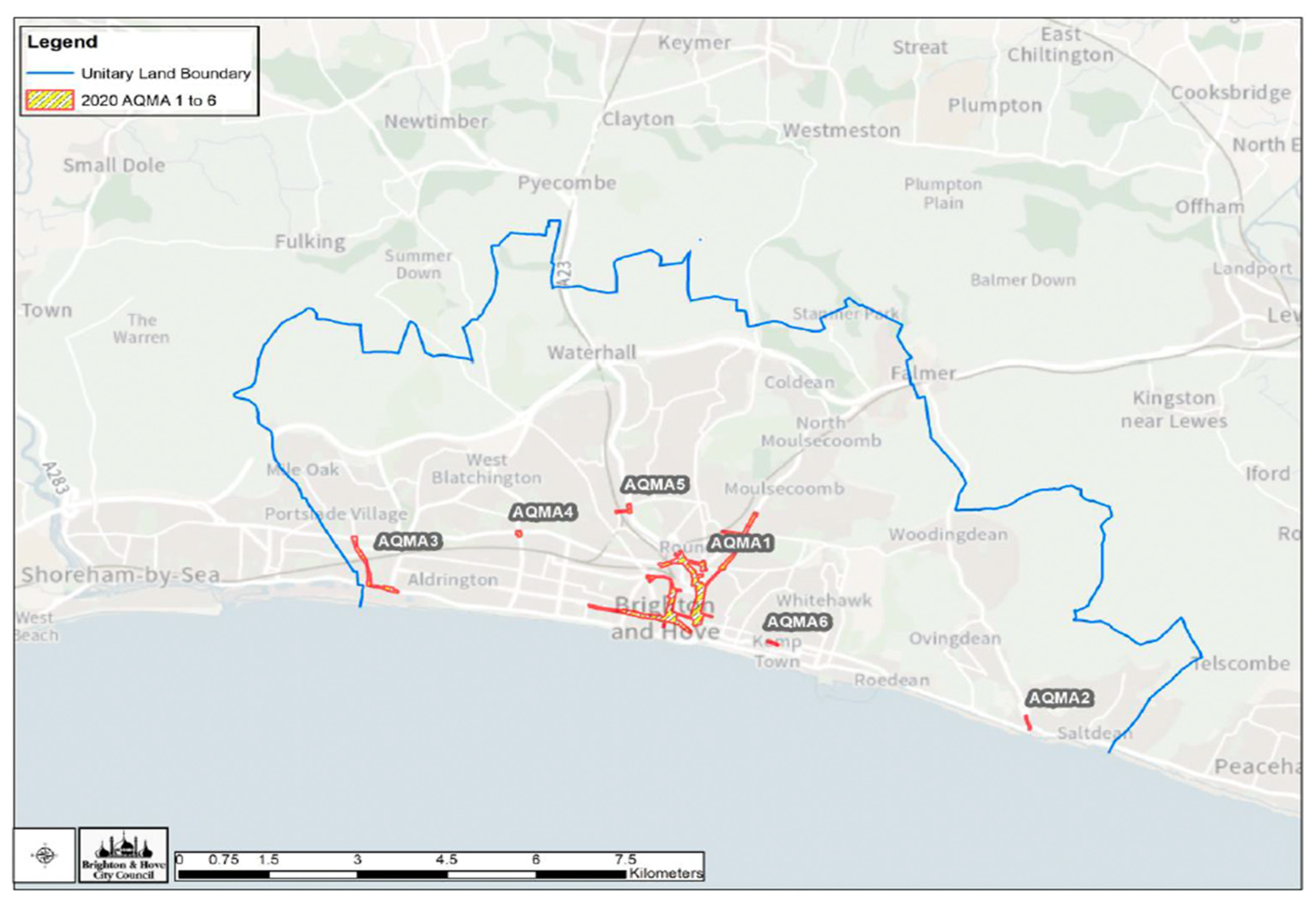
As a densely populated coastal city on the southern coast of England, Brighton and Hove faces persistent air quality challenges driven primarily by vehicular emissions, with NO₂, PM, and SO₂ identified as key pollutants [43]. Despite exposure to relatively clean maritime air, pollution episodes occur during tourist seasons and in high-traffic areas, leading to the designation of Air Quality Management Areas (AQMAs) for NO₂ exceedances (Figure 1) [43,44]. Historical records show that some AQMAs previously exceeded the UK annual mean NO₂ limit of 40 µg/m³, although levels have declined to below 20 µg/m³ by 2023 due to mitigation strategies such as low-emission initiatives, promotion of electric vehicles, and improved public transport [41].

Traditional fixed-site monitoring in Brighton provides valuable data but is limited in spatial coverage and vertical resolution, potentially overlooking local hotspots and pollutant variability [22,45]. Integrating MAX-DOAS and LP-DOAS with satellite observations overcomes these constraints by enabling detailed vertical (MAX-DOAS) and horizontal (LP-DOAS) profiling of atmospheric pollutants, improving understanding of pollutant sources, transport, and transformation processes [46,47,48,49,50,51,52,53,54,55,56,57,58,59,60,61,62,63,64,65]. MAX-DOAS quantifies concentrations at different altitudes and supports assessment of meteorological influences on dispersion [66,67], including wind-driven accumulation and dilution effects [68,69], while satellite remote sensing provides large-scale spatial coverage [70]. Validation of Sentinel-5P TROPOMI data with ground-based measurements enhances data reliability in Brighton. Although such integrated approaches have proven effective in other urban contexts [60,71,72,73,74,75,76], limited research exists for Brighton; incorporating historical MAX-DOAS and LP-DOAS data enables evaluation of long-term trends, seasonal variability, and the effectiveness of past interventions, providing a robust basis for local air quality management.

The primary aim of this research is to employ current and historical MAX-DOAS, LP-DOAS and satellite observations to conduct a thorough atmospheric assessment of NO₂, SO₂, HONO, HCHO, and O₃ pollutants in Brighton from 01/07/2021–22/07/2021; 17/01/2022–05/09/2022; 20/03/2024–25/03/2024; 16/05/2024–20/05/2024. The main objectives include: (i) To assess the spatial and temporal distribution of these pollutants in Brighton; (ii) to analyse diurnal and seasonal trends of these pollutants using integrated data; (iii) to compare ground-based measurements with TROPOMI data for validation and trend analysis; and (iv) to analyse the impact of urban infrastructure on the distribution of pollutants, providing insights into pollution dynamics in Brighton. By conducting a thorough analysis of historical and recent data in Brighton, this research seeks to provide a comprehensive overview of the trends and current status of these pollutants in the city’s troposphere. The integration of these diverse data sources is expected to yield a robust framework for understanding and managing urban air quality in Brighton, contributing valuable insights applicable to other urban settings facing similar challenges.

This paper describes the study area, datasets, instrumentation, and analytical methodology employed in the investigation. It then presents the temporal and spatial characteristics of the measured pollutants and evaluates the performance of Sentinel-5P TROPOMI observations against MAX-DOAS and LP-DOAS measurements. The findings are subsequently discussed in the context of urban atmospheric chemistry and satellite remote sensing, before concluding with the principal findings, study limitations, and recommendations for future research.

2. Materials and Methods

2.1. MAX-DOAS Instrument

The Airyx SkySpec Compact 200 MAX-DOAS instrument (Airyx GmbH, Enviro Technology, Gloucestershire, UK) used for this study is designed to provide detailed and accurate measurements of atmospheric trace gases by leveraging the principles of MAX-DOAS. This advanced remote sensing technique quantifies the concentration of trace gases by analysing the absorption of specific wavelengths of light in the ultraviolet (UV) and visible regions of the solar spectrum [77,78]. The spectral analysis settings and retrieval parameters for MAX-DOAS measurements of trace gases are detailed in

Table 1. Spectral Analysis Settings and Parameters for MAX-DOAS Measurements of Trace Gases.

	NO2	SO2	O3	HONO	BrO	Glyoxal	References
Start Wavelength [nm]	425	315	336	336	332	432
End Wavelength [nm]	498	327	359	373	358	458
Polynomial Degree	4	3	3	3	3	3
NO2 224K	✓		✓	✓	✓	✓	[80]
NO2 294K	✓	✓	✓	✓	✓	✓	[80]
SO2		✓					[81,82]
O3 223K	✓	✓	✓	✓	✓	✓	[83]
O3 243K	✓	✓	✓			✓	[83]
BrO	✓		✓	✓	✓		[84]
HCHO	✓		✓	✓		✓	[85]
HONO	✓		✓	✓	✓	✓	[86]
Glyoxal	✓		✓	✓		✓	[87]

. The instrument works by collecting scattered sunlight using a sophisticated telescope scanner unit. This unit directs the light through a quartz-glass tube and an optical fibre into a spectrometer unit. The spectrometer unit, comprising two temperature-stabilised Avantes spectrometers optimised for UV (295–450 nm) and visible (430–565 nm) light, records the intensity of the light at different elevation angles. This multi-axis scanning approach enhances sensitivity to near-surface concentrations and provides a comprehensive profile of the atmospheric column [79]. This setup minimises stray light and enhances measurement accuracy, with temperature stabilisation ensuring consistent performance.

The core principle of the MAX-DOAS instrument is based on the DOAS technique [79], which measures trace gas concentrations by analysing their differential absorption in the atmosphere. The instrument captures scattered sunlight at multiple elevation angles to provide vertical profiles of gas concentrations.

Light collected by the telescope is dispersed into component wavelengths by the spectrometer and recorded for detailed spectral analysis. Using MS-DOAS software, which controls the instrument, the spectra are processed to identify absorption features unique to each gas, enabling their quantification. The resulting differential absorption spectra are compared to reference spectra to calculate slant column densities (SCDs), which represent the concentration of trace gases along the optical path. SCDs are converted to vertical column densities (VCDs) using air mass factors (AMFs) (Equation (1)), which account for the geometry of the light paths and the distribution of the gases, and depend on factors like the solar zenith angle, the telescope elevation angle, and the azimuth angle. VCDs provide a clear measure of trace gas concentrations in a vertical column.

$$VCD={\displaystyle \frac{dSCD}{AMF}}$$

(1)

Instrument Location and Experimental Set-Up

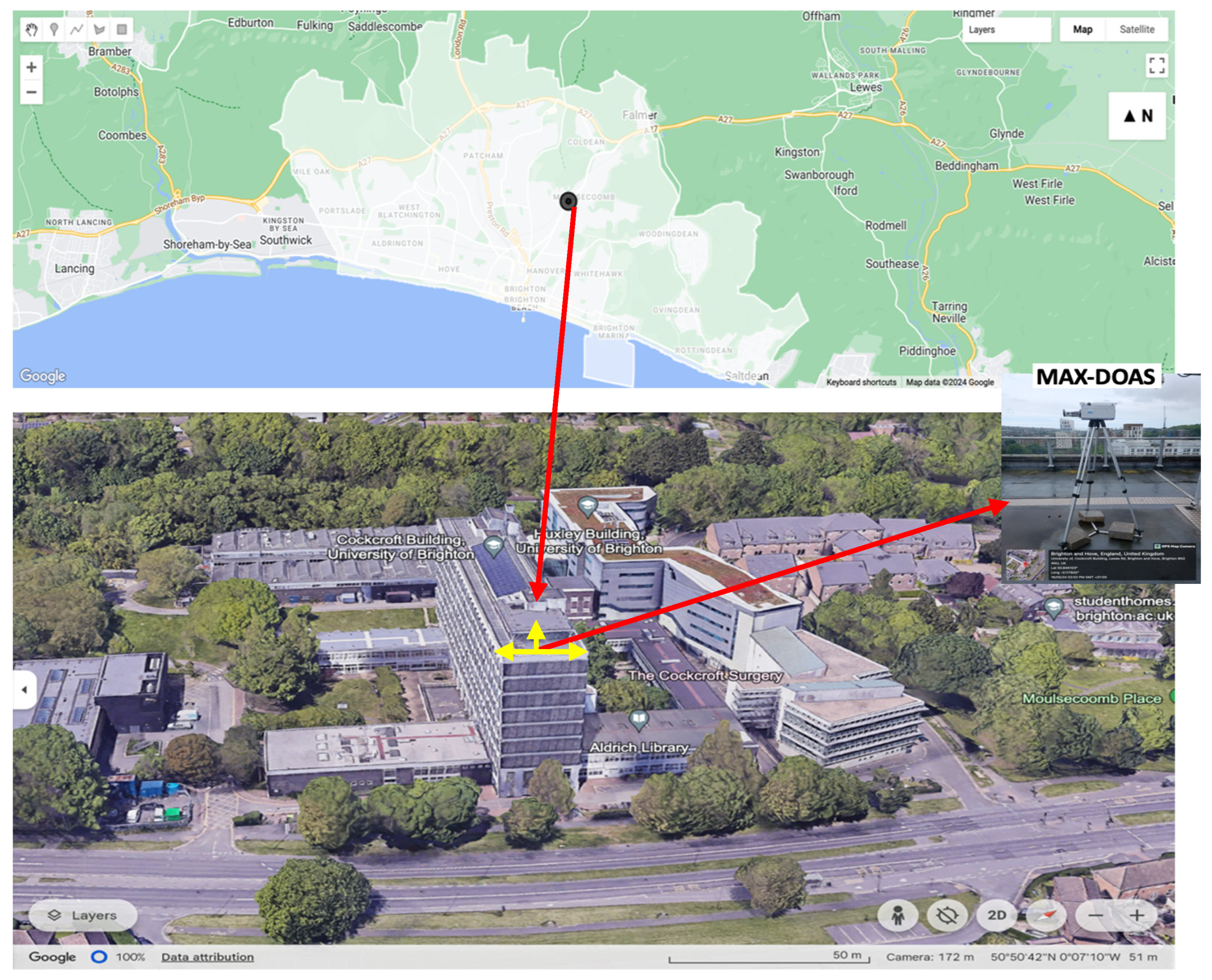
The MAX-DOAS instrument was strategically installed on a tripod mount on the roof of the Cockcroft Building, located at the Moulsecoomb campus of the University of Brighton, UK (Latitude: 50.84517°, Longitude: −0.117862°) (Figure 2). The Cockcroft Building stands approximately 38 m above ground level, providing an elevated vantage point that is essential for unobstructed atmospheric measurements. This elevated position allows for a clear line of sight necessary for capturing comprehensive atmospheric data.

The telescope scanner unit was positioned upright on the mounting plate, with the quartz-glass tube and rotating prism facing the desired viewing direction (North and South). The site is situated within a residential urban area, approximately 2 km from Brighton’s city centre and seafront and 5 km from Falmer on the A27 road, making it ideal for capturing data relevant to both urban and coastal influences on air quality. The site is adjacent to the A270 Lewes Road, a busy thoroughfare that connects northwards to the A27 at Falmer. This road is a significant route that experiences high traffic volumes, contributing to substantial vehicular emissions. This provides an optimal setting to study the impact of traffic emissions. Furthermore, the site location is characterised by a mix of residential homes, industrial activity, and significant traffic flow, contributing to diverse emission sources. The residential areas around the site introduce typical urban emissions from domestic activities, while the industrial activities add another layer of complexity to the local air pollution scenario. Additionally, the area features fields, forests, and allotments situated at the top of the valley, offering a unique opportunity to study the interplay between urban emissions and natural landscapes.

2.2. LP-DOAS

The LP-DOAS instrument is a powerful tool used for measuring trace gas concentrations in the atmosphere. The instrument setup involves a broad-spectrum light source, such as a Xenon lamp, that sends a light beam along a defined path through the atmosphere to a receiver, typically equipped with a spectrometer. As the light travels through the atmosphere, it interacts with gas molecules, which absorb specific wavelengths, creating characteristic absorption features in the received spectrum.

The LP-DOAS technique employs differential absorption, comparing the measured spectrum to a reference spectrum taken at a different time or under idealised laboratory conditions to isolate and quantify the absorption due to target gases using the DOAS method [88].

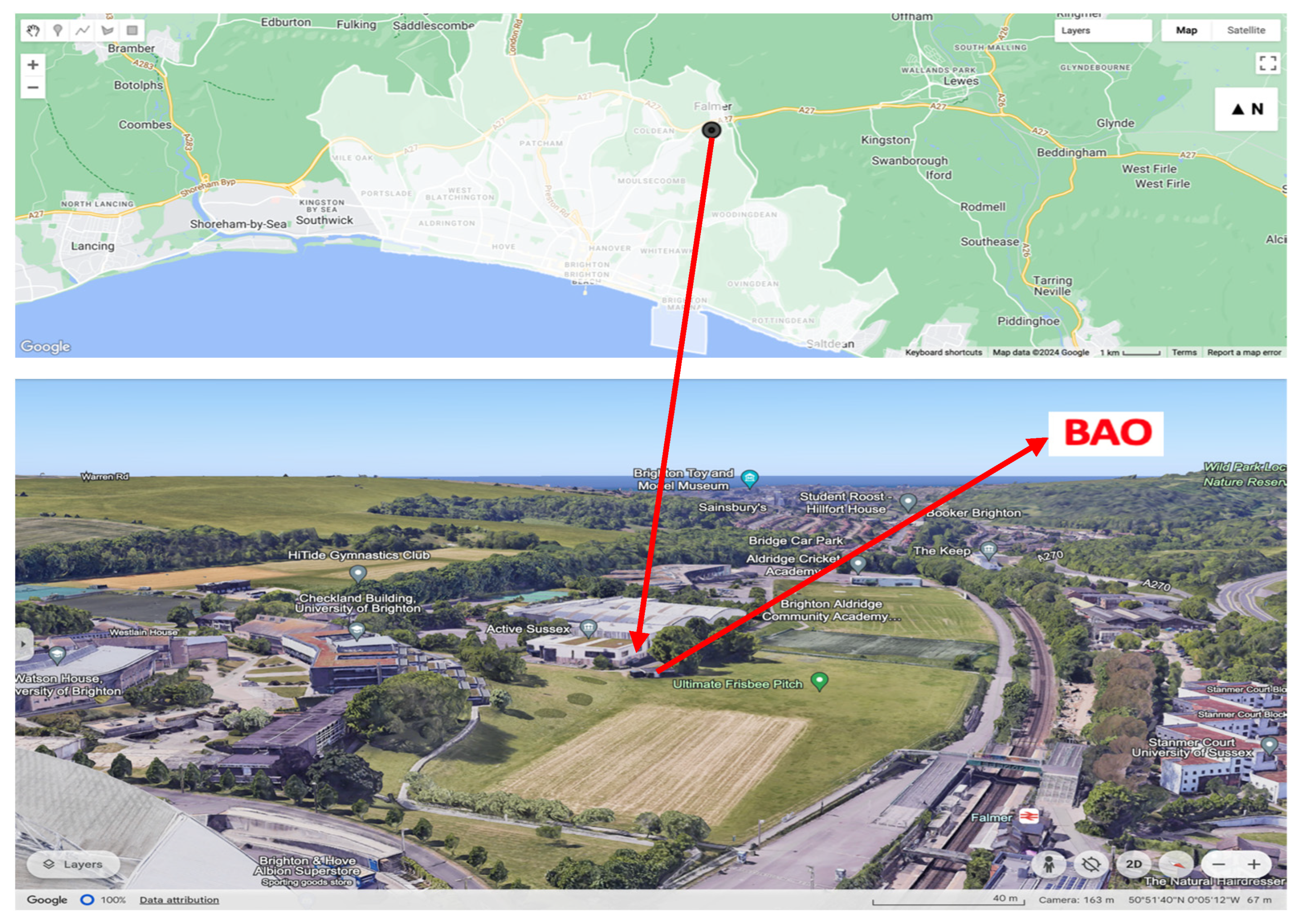
The LP-DOAS historical data were obtained using an Opsis AB Model ER120 Transceiver and System 300 Spectrometer LP-DOAS instrument (Opsis AB, Enviro Technology, Gloucestershire, UK) installed at the Brighton Atmospheric Observatory (BAO) at coordinates 50.860312, −0.088179 (Figure 3). Established in 2015 as part of the EU Joint Air Quality Initiative (JOAQUIN), BAO is managed by the University of Brighton’s Centre for Earth Observation Science (CEOBS). Located on the university’s Falmer campus, the observatory is in a semi-suburban setting with the South Downs National Park to the north and Brighton and Hove, along with the English Channel, to the south. This strategic location, about 4.5 km from the city centre and 5.5 km from the coast, is ideal for studying air quality in the populous South-East UK, between the pollution hotspots of London and northwest Europe [89].

2.3. Sentinel-5P Tropospheric Monitoring Instrument

The Sentinel-5P Tropospheric Monitoring Instrument (TROPOMI) is a state-of-the-art spectrometer aboard the European Space Agency’s (ESA) Sentinel-5 Precursor (S-5P) satellite, which is part of the Global Monitoring for Environment and Security (GMES) program. The instrument operates in a sun-synchronous orbit, providing daily global coverage that is critical for comprehensive air quality monitoring [90]. Launched to enhance our understanding of atmospheric composition, TROPOMI covers a spectral range from the ultraviolet (UV) to the shortwave infrared (SWIR). This wide spectral coverage allows it to measure and monitor various key atmospheric pollutants such as O₃, NO₂, SO₂, CO, CH₄, CH₂O, and aerosols, all with a high spatial resolution of 3.5 × 5.5 km² at nadir. TROPOMI can identify moderate-sized pollution sources, including cities, power plants, industrial areas, major highways, individual fires, and even single large ships [73,91,92,93,94]. The instrument serves as a critical component in the methodology of this research. For this study, pollutant distributions observed through MAX-DOAS and LP-DOAS were utilised to validate and enhance the spatial and temporal understanding of the satellite observations from Sentinel-5P in Brighton, UK.

2.4. Data Collection and Analysis Techniques

The methodology for analysing and validating TROPOMI data using MAX-DOAS and LP-DOAS data, incorporating both historical and current data, involves a systematic process of data collection, pre-processing, analysis, and comparison. Specifically, the study compared tropospheric VCDs of pollutants retrieved from TROPOMI with corresponding measurements obtained from ground-based MAX-DOAS and LP-DOAS instruments installed at the atmospheric monitoring sites in Brighton. This comprehensive approach ensures that the data collected is representative of long-term trends and immediate air quality challenges faced by Brighton. The initial step involves accessing the historical LP-DOAS data from the BOA archive and downloading the relevant historical and current Sentinel-5P TROPOMI data for the same period as the MAX-DOAS and LP-DOAS observations using Google Earth Engine (GEE), a powerful tool for accessing and processing large-scale geospatial datasets. This ensures that the data covers the geographic area of the instruments and spans a sufficient timeframe to capture seasonal variations and long-term trends. The overall temporal availability of the datasets is summarised in

Table 2. Summary of datasets used in this study, including their sources, characteristics, quality control criteria, and temporal coverage.

Instrument	Data Type	Observation Period	Data Provider	Source	Data Format	Temporal Frequency	Spatial Resolution	QA Criteria	Update Frequency
MAX-DOAS	Ground-based observations	01 Jul 2021–22 Jul 2021	BAO	BAO archive/campaign observations	CSV	Hourly	Point measurement (vertical column retrieval)	Quality-controlled spectra; invalid retrievals removed	Campaign-based
		17 Jan 2022–05 Sep 2022
		20 Mar 2024–25 Mar 2024
		16 May 2024–20 May 2024
LP-DOAS	Ground-based observations	05 Aug 2015–01 Jun 2023	BAO		CSV	Hourly	~1 km optical path	negative values removed	Continuous
TROPOMI	Satellite observations	Extracted for the same periods as MAX-DOAS and LP-DOAS	ESA Sentinel-5P (via GEE)	GEE/Copernicus	GeoTIFF/NetCDF (processed to CSV)	Daily overpass	3.5 × 5.5 km2 (nadir)	QA ≥ 0.75; negative values removed	Daily

.

To ensure spatial consistency between satellite and ground-based observations, an Area of Interest (AOI) centred on the geographic coordinates of the measurement instruments was defined. A 5 km buffer was applied around the MAX-DOAS instrument and a 1 km buffer around the LP-DOAS instrument. These buffers represent the approximate observational footprint of the instruments and allow the satellite data to better reflect local pollutant concentrations.

Prior to analysis, all datasets were pre-processed to ensure consistency and quality by standardising timestamps to Coordinated Universal Time (UTC) and aligning observations temporally to enable direct comparison between satellite overpasses and ground-based measurements, while retaining only coincident data within the study period. Missing values, arising from factors such as instrument downtime and cloud cover, were handled by excluding incomplete records from correlation and regression analyses to avoid bias. For time-series visualisation, internal missing values were estimated using linear interpolation to provide continuous temporal profiles, whereas leading and trailing missing values were retained as missing, as interpolation cannot reliably estimate values beyond the observed data range. Additionally, quality control measures were applied, including the removal of non-physical values and the use of TROPOMI quality assurance (QA) flags, to ensure the reliability of the datasets.

For TROPOMI data, further preprocessing steps were applied to enhance data quality and usability. Mean pollutant concentrations within the AOI were calculated at hourly resolution to provide detailed temporal profiles. Negative values, which may arise from sensor noise or retrieval uncertainties, were removed. A QA filtering threshold of 0.75 was applied to the tropospheric NO₂ column number density to retain only high-quality pixels, excluding those affected by cloud contamination or retrieval errors. Following quality filtering, pollutant VCDs were converted from mol/m² to molecules/cm² using Equation (2), ensuring consistency in units for analysis. The processed datasets were then formatted with standardised timestamps and exported as CSV files for subsequent analysis in RStudio (version 2024.04.1), using the OpenAir package.

$$VDC in \mathrm{m}\mathrm{o}\mathrm{l}\mathrm{e}\mathrm{c}\mathrm{u}\mathrm{l}\mathrm{e}\mathrm{s}/{\mathrm{c}\mathrm{m}}^2 = VDC in \mathrm{m}\mathrm{o}\mathrm{l}/{\mathrm{m}}^2 \times 6.022 \times {10}^{19}$$

(2)

In parallel, historical and current MAX-DOAS and LP-DOAS datasets were pre-processed using Microsoft Excel before import into RStudio. This involved formatting timestamps and pollutant variables, as well as aggregating data where necessary to match the temporal resolution of TROPOMI observations, ensuring consistency across datasets.

Uncertainties associated with each observation platform were considered during data integration. For MAX-DOAS, these include spectral fitting errors, instrumental stability, and uncertainties in AMF calculations, while LP-DOAS measurements may be affected by uncertainties related to spectral retrieval, instrument stability, and atmospheric variability along the optical path. TROPOMI uncertainties are associated with retrieval algorithms, cloud effects, and differences in spatial resolution compared with ground-based observations. Error propagation during dataset integration was addressed through quality control procedures, including removal of invalid observations, TROPOMI QA filtering, spatial averaging within defined areas of interest, and temporal matching of coincident measurements. The influence of residual uncertainties was evaluated through correlation, regression, and bias analyses.

Subsequently, statistical and computational analyses were conducted to compare the datasets. Temporal alignment was achieved by synchronising ground-based observations with satellite overpass times. Statistical metrics, including correlation, bias, and error analysis, were used to evaluate the consistency and reliability of the measurements. Time series plots were generated to assess temporal variability and agreement between datasets, alongside time variation plots capturing diurnal and seasonal trends. Additionally, polar plot analysis was performed to examine relationships between pollutant concentrations and meteorological conditions. Meteorological data were obtained from the Shoreham Met Station, UK, using the worldmet package in RStudio. Shoreham Met Station provides the nearest continuous, quality-controlled meteorological observations and was considered representative of the regional meteorological conditions during the study period. This comprehensive approach integrates both historical and current satellite and ground-based observations, enhancing the accuracy and reliability of atmospheric monitoring in urban settings like Brighton.

3. Results and Discussions

3.1. LP-DOAS Measurements

3.1.1. Overview of Historical Pollutant Concentration

The analysis of the overall historical LP-DOAS data collected at BAO, as shown in

Table 3. Summary statistics for the historical pollutant (µg/m³) measured by the Long-Path DOAS instrument at BAO from 05/08/2015 to 01/06/2023, and meteorological data from Shoreham Met-Station, UK, from 01/01/2017 to 01/06/2023.

Season	Statistics	NO2	SO2	HCHO	HONO	O3	ws (ms−1)	wd ° (North)	TP (°C)	RH (%)
Autumn	Mean	20.11	1.71	7.43	2.60	44.81	4.78	219.65	12.30	85.01
(N = 16,556)	Median	14.51	1.55	6.89	2.23	46.41	4.27	230.00	12.70	87.07
	St. dev.	17.44	0.85	3.47	1.52	19.65	2.73	102.32	4.47	10.79
	Min.	0.03	0.09	0.68	0.00	1.98	0.00	0.00	−2.50	35.31
	Max.	178.40	14.58	29.45	12.68	122.1	20.10	360.00	26.17	100
Spring	Mean	16.21	1.75	8.53	2.39	63.34	4.65	186.15	9.92	79.87
(N = 15,389)	Median	11.46	1.63	8.15	2.27	65.53	4.27	200.00	9.87	82.44
	St. dev.	14.91	0.87	3.31	0.98	21.36	2.55	112.49	4.14	13.94
	Min.	0.06	0.26	0.074	0.00	3.18	0.00	0.00	−4.00	27.10
	Max.	144.95	19.05	24.75	7.93	146.12	16.13	360	25.87	100
Summer	Mean	13.31	1.76	8.30	2.37	55.42	4.53	209.46	17.21	79.36
(N = 14,611)	Median	9.87	1.58	7.70	2.16	54.33	4.10	220.00	17.20	81.51
	St. dev.	11.56	1.45	3.71	1.18	22.68	2.57	100.08	3.60	13.56
	Min.	0.087	0.39	1.08	0.00	3.24	0.00	0.00	4.60	27.10
	Max.	122.63	123.79	31.82	8.82	178.38	15.63	360.00	33.00	100
Winter	Mean	23.20	1.69	7.99	2.81	49.04	4.98	215.28	6.16	87.80
(N = 15,823)	Median	15.48	1.57	7.57	2.56	51.49	4.60	230.00	7.00	89.86
	St. dev.	21.69	0.78	3.07	1.43	20.41	2.88	99.99	3.75	9.52
	Min.	0.02	0.11	0.70	0.00	0.90	0.00	0.00	−6.20	35.19
	Max.	239.88	27.61	34.45	10.75	96.07	20.23	360.00	14.70	100
ALL	Mean	18.34	1.72	8.05	2.56	52.91	4.74	206.95	11.25	82.98
(N = 62,379)	Median	12.48	1.58	7.57	2.30	54.018	4.27	223.10	11.00	85.74
	St. dev.	17.32	1.02	3.42	1.32	22.15	2.69	104.94	5.64	12.64
	Min.	0.02	0.09	0.07	0.00	0.9	0.00	0.00	−6.20	27.10
	Max.	239.88	123.79	34.45	12.68	178.38	20.23	360.00	33.00	100

N is the sample size (averaged hourly).

, reveals significant insights into the variability of the measured atmospheric pollutants. The data show that NO₂ has an overall mean concentration of 18.34 (±17.32) µg/m³, which is below the EU and UK annual mean limit of 40 µg/m³. However, there is substantial variability with occasional extreme hourly values reaching up to 239.88 µg/m³, exceeding the EU and UK hourly limit of 200 µg/m³, likely due to a short-term episodic spike [95,96]. SO₂, with a mean concentration of 1.72 (±1.02) µg/m³, exhibits less variability, suggesting fewer major sources in the area. HCHO has a mean concentration of 8.05 (±3.42) µg/m³. HONO levels average 2.56 (±1.32) µg/m³, showing significant peaks during specific conditions. O₃ levels, averaging 52.91 (±22.15) µg/m³, demonstrate considerable variability with peaks up to 178.38 µg/m³ during periods of high photochemical activity.

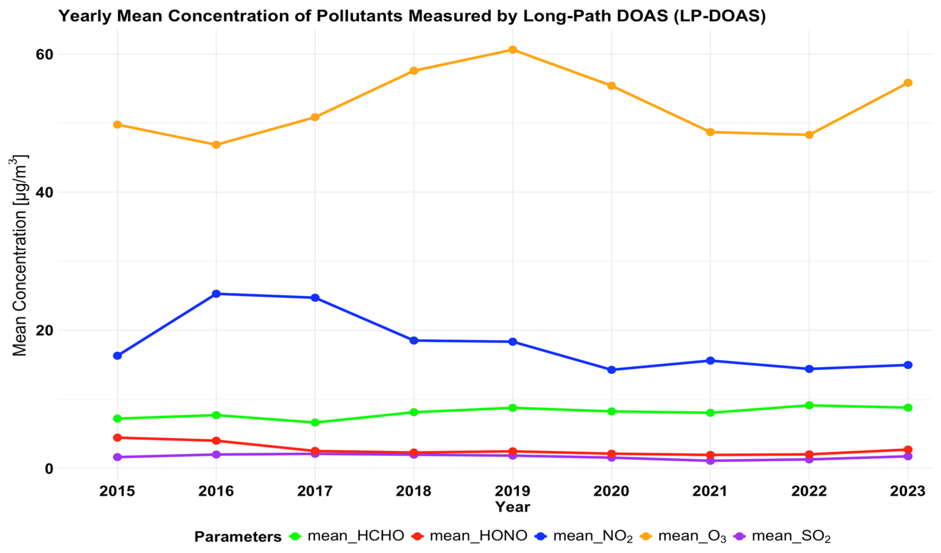
The analysis of yearly mean concentrations of the pollutants reveals significant fluctuations, reflecting the dynamic nature of urban pollution (Figure 4). NO₂ levels peaked in 2016 at 25.28 µg/m³ before stabilising around 14–15 µg/m³ from 2020 onwards, indicating the potential effectiveness of emission control measures. SO₂ remained low with minor variations, showing a downward trend likely due to improved industrial emission controls. HCHO levels exhibited a general upward trend, peaking at 9.11 µg/m³ in 2022, suggesting increased photochemical activity.

HONO showed no clear trend, varying between 1.93 and 4.43 µg/m³, influenced by complex emission and formation processes. O₃ concentrations fluctuated significantly, with peaks in 2019 and 2023, but generally remained below the UK 3-year average 8 h mean concentration of 120 µg/m³ [97], underscoring the need to understand and manage precursor emissions and atmospheric conditions.

3.1.2. Seasonal and Diurnal Variation of Pollutants Measured by LP-DOAS

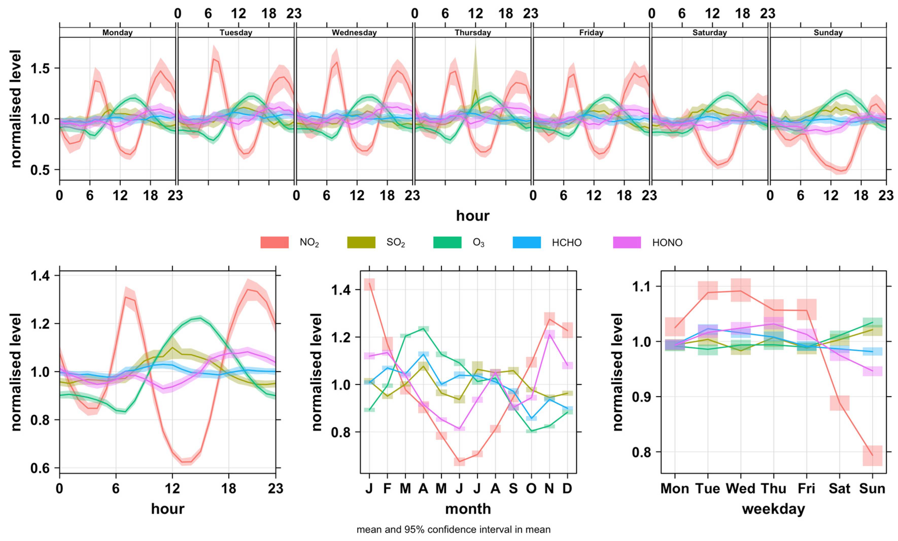
The normalised time-variation plot (Figure 5) presents the comparative temporal behaviour of NO₂, SO₂, O₃, HCHO, and HONO measured at Falmer, Brighton, between 2015 and 2023. The combined representation allows direct comparison of seasonal, diurnal, and weekday patterns across pollutants, highlighting differences driven by emission sources and atmospheric chemistry.

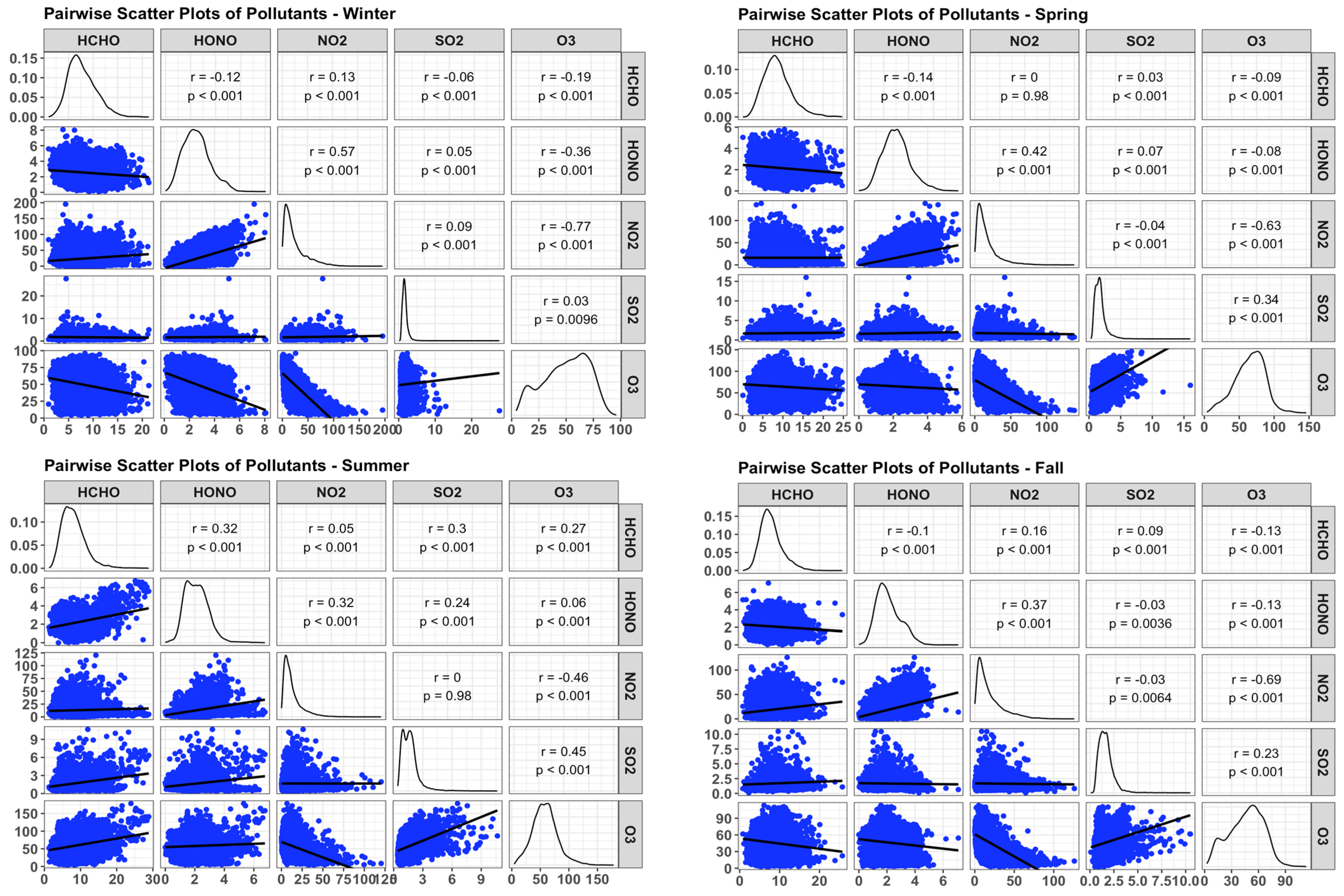
Distinct variations are evident between primary emitted pollutants and those formed through secondary photochemical processes. The diurnal patterns show clear contrasts between primary pollutants and secondary species. NO₂ exhibits a pronounced bimodal distribution with peaks during the morning (~06:00–09:00) and evening (~18:00–22:00) hours, corresponding to increased vehicular emissions during commuting periods, which is consistent with observations reported for urban UK sites and other cities [98,99,100,101,102]. HONO shows similar behaviour with enhanced concentrations during nighttime and early morning periods, reflecting accumulation under reduced photolysis conditions and formation through heterogeneous reactions involving NO₂ and surface processes [40,103,104]. This relationship is reflected in the moderate positive winter correlation between HONO and NO₂ (r = 0.57) (Figure 6), indicating common emission sources and coupled secondary formation pathways [104]. In contrast, O₃ and HCHO display opposite daytime behaviour, characterised by increases during late morning and midday when solar radiation is strongest. These trends indicate their formation through photochemical oxidation of VOCs and NOx in the presence of sunlight [38,39,42,105,106,107]. O₃ typically reaches maximum concentrations from midday to early afternoon (~12:00–16:00), which is consistent with photochemical production mechanisms widely reported in urban and coastal environments [108,109,110,111].

HCHO also shows daytime enhancement associated with secondary formation from VOC photo-oxidation, a process known to dominate global HCHO sources [38,105,106,107]. SO₂ exhibits comparatively weaker diurnal variability, reflecting its relatively low concentrations and mixed sources, including combustion processes and regional transport [34].

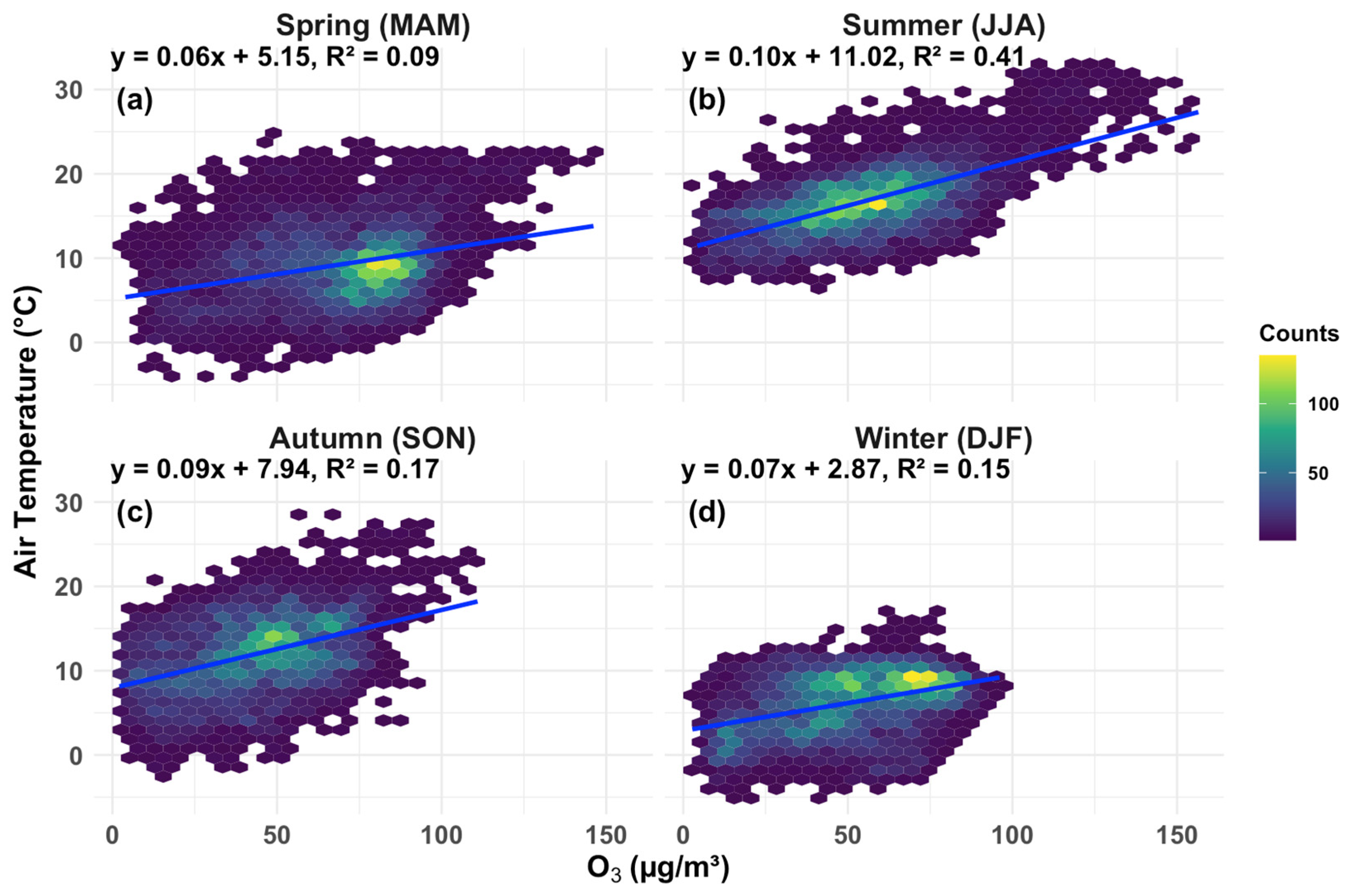
Seasonal and monthly variations further highlight the contrasting atmospheric processes controlling these pollutants. O₃ and HCHO generally show higher levels during spring and summer, consistent with increased photochemical activity driven by higher temperatures, stronger solar radiation, and increased emissions of BVOCs from vegetation [38,71,112]. This behaviour is supported by the observed positive association between O₃ and air temperature (Figure 7) (R² = 0.41 in summer), while a weaker relationship is observed during winter (R² = 0.15), likely due to reduced photochemical activity and lower solar radiation [113]. Conversely, NO₂ and HONO tend to show relatively higher levels during autumn and winter when increased combustion emissions from traffic and heating, combined with lower boundary layer heights and weaker photolysis, favour pollutant accumulation [40,103,104,114,115]. A moderate positive correlation between HONO and NO₂ during winter (r = 0.57) (Figure 6) further indicates shared emission sources and secondary formation pathways involving NO₂ chemistry [104].

Similar seasonal behaviour has been reported in several urban environments across the UK and other Urban cities [116,117,118,119,120]. NO₂ shows an inverse relationship with O₃, particularly during winter (r = −0.77) and summer (r = −0.46) (Figure 6), reflecting the well-known titration effect where elevated NO₂ suppresses O₃ concentrations under reduced photochemical activity [39,42]. SO₂ shows comparatively small seasonal variation, reflecting the substantial long-term decline in emissions in the UK due to stricter environmental regulations and transitions toward cleaner energy sources, which have resulted in an overall reduction of approximately 99% in emissions [121,122,123]. The weekday analysis further highlights the influence of anthropogenic activities, with slightly higher NO₂ and HONO levels during weekdays compared with weekends due to traffic-related emissions, while O₃ occasionally shows modest weekend enhancements consistent with the commonly observed urban “weekend effect” reported in other studies [124,125,126].

Overall, the comparative temporal behaviour of the pollutants highlights the interplay between emission sources and atmospheric photochemistry in shaping urban air quality. Primary pollutants such as NO₂ and HONO are largely controlled by traffic and combustion activities and therefore show stronger nighttime or rush-hour peaks, whereas secondary pollutants such as O₃ and HCHO are mainly driven by daytime photochemical reactions involving precursor gases. These findings are consistent with previous observations from urban and coastal environments where the balance between anthropogenic emissions, photochemical production, and meteorological conditions governs pollutant variability [39,42,108,109,110].

3.1.3. Effect of Wind Speed and Wind Direction on Seasonal Variation of Pollutants

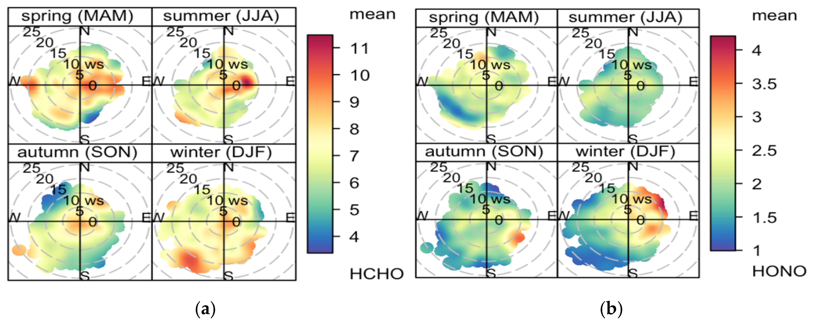
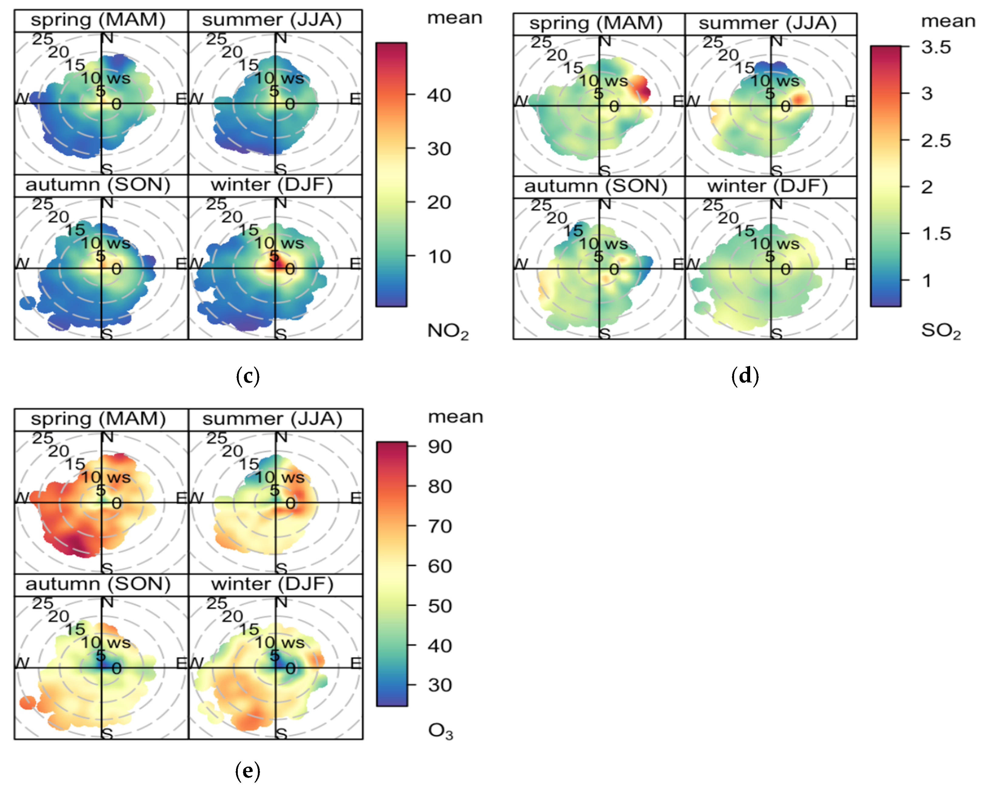
The polar plots (Figure 8) for each pollutant provide insights into the sources and transport mechanisms affecting pollutant concentrations across all seasons. During spring, high HCHO levels were observed (Figure 8a) with moderate winds (up to 15 m/s) from the west and southeast, suggesting both local sources of VOCs, possibly from vehicular exhaust from the busy A270 Lewes Road, which has been reported to carry over 25,000 cars daily [127], and regional transport. In summer, peak HCHO levels were associated with winds from the east and southeast at moderate speeds (<15 m/s), likely driven by enhanced photochemical activity from BVOC sources due to higher temperatures and increased sunlight. Conversely, winter shows intermediate HCHO levels with winds predominantly from the southwest and southeast at moderate speeds, reflecting reduced photochemical activity and cooler temperatures. HONO concentrations also reveal a distinct relationship (Figure 8b). During spring, intermediate HONO levels are observed with moderate winds (up to 15 m/s) from the north and northwest, likely due to vehicular emission sources. In summer, HONO levels decrease with low-speed southwest winds.

This reduction is likely due to increased photochemical activity breaking down HONO under higher temperatures and sunlight. Autumn shows high HONO levels with winds from the southeast, suggesting a mix of sources. Winter exhibits higher HONO levels with winds from the northeast and southeast at moderate speeds, possibly reflecting increased heating emissions and reduced photochemical activity.

Primary combustion-related pollutants such as NO₂ and SO₂ show patterns influenced by local emissions and atmospheric dispersion. NO₂ concentrations are highest during winter under low wind speeds (<5 m/s) from the north and northeast (Figure 8c), indicating contributions from local traffic emissions, possibly influenced by the nearby A27 motorway, along with domestic heating and reduced atmospheric mixing.

During spring, summer, and autumn, NO₂ levels are generally lower and more evenly distributed across wind directions, reflecting improved atmospheric dispersion. Similarly, SO₂ concentrations remain relatively low overall (Figure 8d), consistent with long-term emission reductions in the UK. Moderate SO₂ levels observed in spring with northeast winds likely suggest contributions from industrial sources and regional transport, while autumn and winter levels associated with southeast and northeast winds likely reflect mixed contributions from domestic heating and fuel combustion.

In contrast, O₃ exhibits patterns strongly linked to photochemical production and regional transport (Figure 8e). Higher O₃ concentrations occur in spring with winds from the southwest and west, and during summer with winds from the east and northeast at moderate speeds, reflecting enhanced photochemical formation involving VOCs and NOx under favourable sunlight and temperature conditions. Lower concentrations observed in autumn and winter are associated with stronger southwest winds (>15 m/s), suggesting transport from cleaner air masses combined with reduced local photochemical production.

3.2. Max-Doas Measurements

3.2.1. Overview of Current and Historical Pollutant Column Densities

The analysis of the current and historical MAX-DOAS data for NO₂ and HONO column densities in Moulsecoomb (

Table 4. Summary statistics for the historical and current pollutant (molecules/cm²) measured by the MAX-DOAS instrument at 20° viewing elevation angle, and metrological data from Shoreham Met-Station, UK, for the periods 01/07/2021 to 22/07/2021, 17/01/2022 to 05/09/2022, and 20/03/2024 to 25/03/2024, and 16/05/2024 to 20/05/2024.

Season	Statistics	NO2	HONO	ws (ms−1)	wd ° (North)	TP (°C)	RH (%)
Spring	Mean	5.02 × 1015	2.76 × 1014	4.82	156.39	9.97	79.85
(N = 385)	Median	4.27 × 1015	1.25 × 1014	4.77	130.00	9.90	82.15
	St. dev.	3.34 × 1015	5.05 × 1014	1.93	91.47	3.26	12.91
	Min.	4.04 × 1014	4.10 × 1012	0.50	0.53	0.40	39.91
	Max.	2.92 × 1016	7.18 × 1015	9.47	360.00	20.20	100.00
Summer	Mean	5.94 × 1015	4.74 × 1015	4.78	199.82	19.26	71.73
(N = 1452)	Median	4.61 × 1015	3.56 × 1015	4.60	210.00	19.42	72.34
	St. dev.	4.56 × 1015	4.11 × 1015	2.02	93.55	3.68	15.06
	Min.	2.49 × 1014	2.86 × 1012	0.00	0.08	6.90	28.97
	Max.	3.26 × 1016	2.28 × 1016	11.80	360.00	31.90	100.00
Winter	Mean	5.04 × 1015	3.05 × 1014	5.40	235.46	7.76	80.36
(N = 365)	Median	4.07 × 1015	1.56 × 1014	4.80	245.66	8.17	81.73
	St. dev.	3.17 × 1015	3.93 × 1014	2.59	77.49	2.73	11.18
	Min.	9.14 × 1014	2.56 × 1012	0.83	7.05	−2.63	40.02
	Max.	2.54 × 1016	4.04 × 1015	13.15	360.00	13.93	99.56
All	Mean	5.62 × 1015	3.23 × 1015	4.86	197.54	15.85	74.71
(N = 2266)	Median	4.50 × 1015	1.89 × 1015	4.60	210.00	17.15	76.03
	St. dev.	4.22 × 1015	3.91 × 1015	2.12	94.08	6.01	14.60
	Min.	2.49 × 1014	2.56 × 1012	0.00	0.08	−2.63	28.97
	Max.	3.26 × 1016	2.28 × 1016	13.15	360.00	31.90	100.00

N is the sample size (averaged hourly).

), measured at a 20° viewing elevation angle, reveals significant variability, with the overall mean values of 5.62 × 10¹⁵ (±4.22 × 10¹⁵) molecules/cm² for NO₂ and 3.23 × 10¹⁵ (±3.91 × 10¹⁵) molecules/cm² for HONO. The substantial standard deviations relative to the means indicate considerable fluctuations in both pollutant levels, suggesting that their levels are heavily influenced by localised emission sources and environmental conditions. The high variability in NO₂ points to the impact of urban activities such as traffic emissions, while the even greater variability in HONO highlights the episodic nature of HONO formation, likely due to both direct emissions and secondary processes involving NO₂. These observations are consistent with findings from other urban studies across Europe, where traffic emissions are a dominant source of NO₂, and HONO formation is closely linked to local NO₂ levels [56,73].

3.2.2. Seasonal and Diurnal Variation of Pollutants Measured by MAX-DOAS

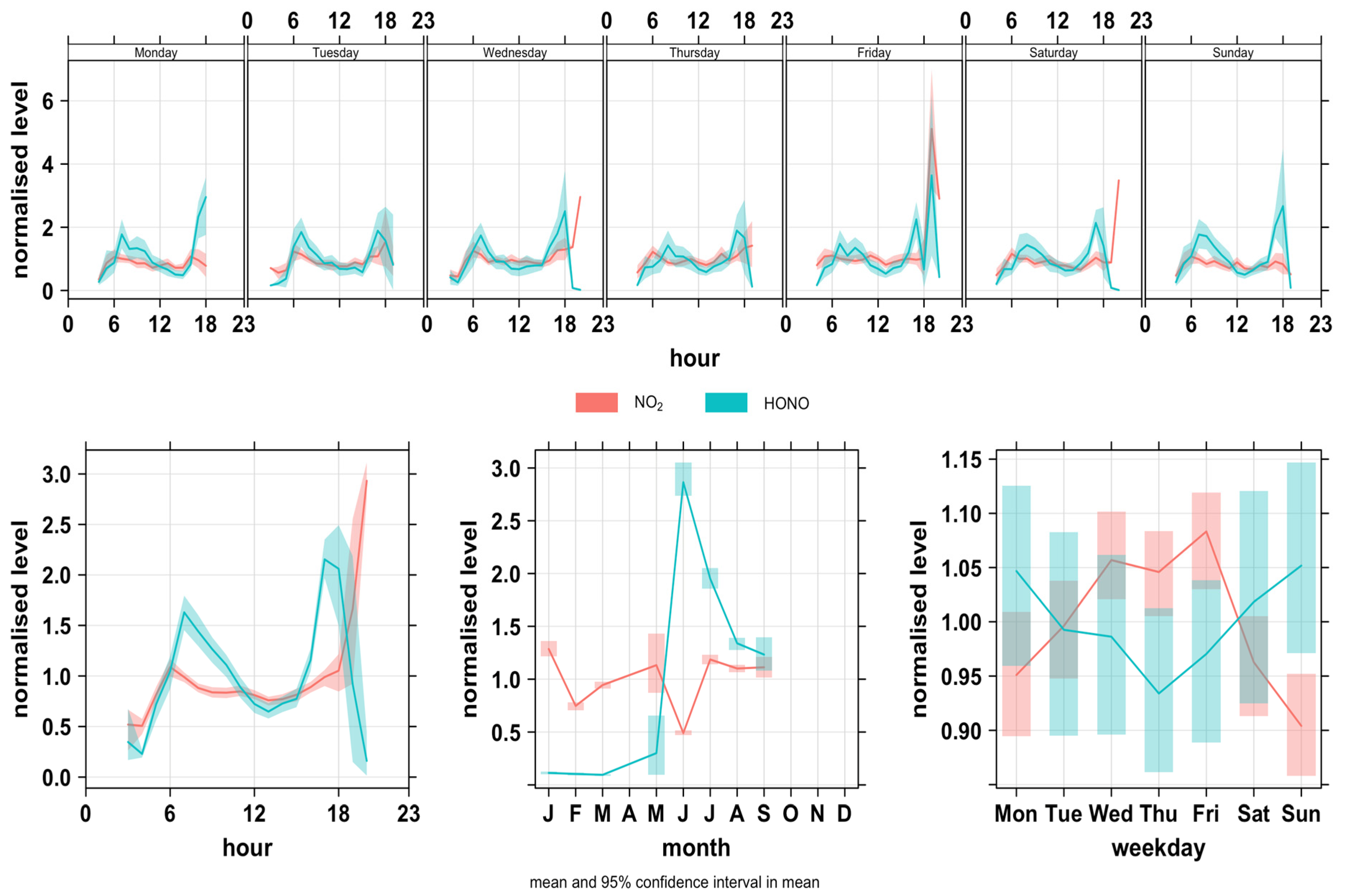
The normalised time-variation plot for NO₂ and HONO measured in Moulsecoomb, Brighton (Figure 9) highlights their comparative seasonal, diurnal, and weekly behaviour.

Presenting both pollutants on a common normalised scale allows direct comparison of their temporal patterns and provides insight into their shared emission sources and chemical interactions. Overall, both pollutants exhibit similar temporal characteristics, reflecting the strong coupling between primary emissions and secondary atmospheric processes that influence urban nitrogen chemistry.

The diurnal patterns reveal a clear bimodal distribution for both pollutants, with enhanced levels during the morning (~06:00–09:00) and evening (~18:00–21:00) periods. These peaks coincide with commuting hours and are strongly associated with vehicular emissions from major roads such as the A270 Lewes Road, a major traffic corridor in the Moulsecoomb area. Similar bimodal patterns have been widely reported for urban environments and are typically attributed to increased traffic activity combined with reduced atmospheric mixing during these periods [101,128,129]. HONO exhibits behaviour comparable to NO₂, particularly during early morning and evening hours, reflecting its close chemical relationship with NO₂. This suggests that HONO formation is partly driven by heterogeneous conversion of NO₂ on urban surfaces in addition to direct emissions. During daytime, especially around midday, HONO abundance decreases due to enhanced photolysis under stronger solar radiation, which converts HONO into hydroxyl radicals (OH).

Seasonal variability further reflects the influence of emission sources and meteorological conditions on pollutant accumulation. NO₂ generally shows relatively elevated levels during colder months due to increased combustion emissions and reduced boundary layer heights that limit pollutant dispersion, although the seasonal trend remains uncertain due to limited winter measurements. HONO shows less pronounced seasonal variability but generally follows NO₂ behaviour due to their chemical linkage.

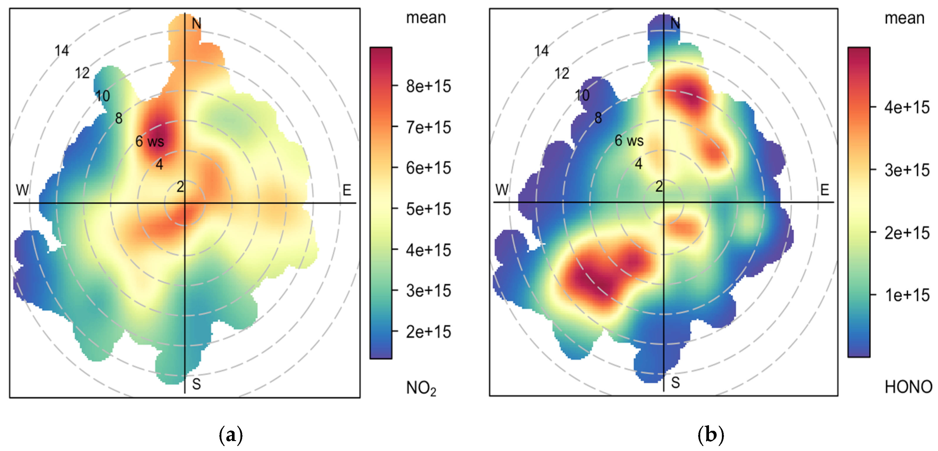
Wind analysis (Figure 10a) indicates that elevated NO₂ abundance is primarily associated with low wind speeds (<8 m s⁻¹) and air masses arriving from the north-west, likely reflecting vehicular emissions from the nearby A270 Lewes Road. In contrast, higher HONO levels occur mainly under moderate wind speeds (<10 m s⁻¹) from the north-east and south-west directions (Figure 10b), suggesting contributions from nearby traffic corridors as well as potential local sources such as rail activity or residential combustion. These conditions favour pollutant accumulation and highlight the role of wind direction and speed in controlling the dispersion and local build-up of nitrogen-related pollutants in the Moulsecoomb area.

3.2.3. MAX-DOAS Comparison with LP-DOAS Data

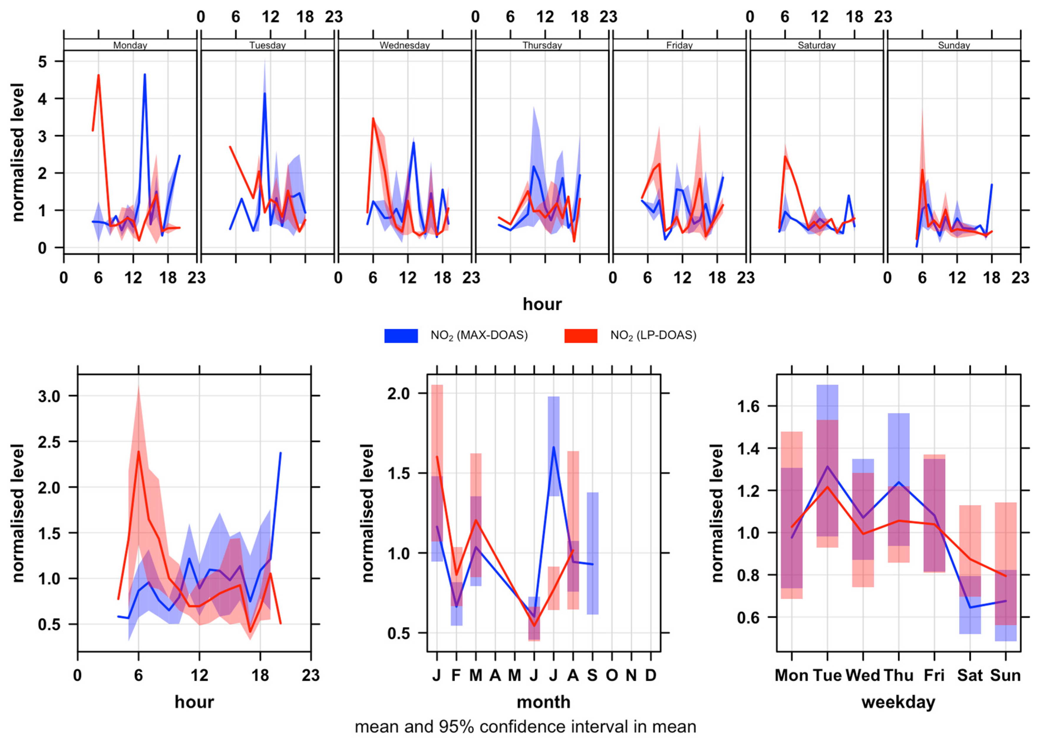
Figure 11 presents a comparison of NO₂ measurements obtained from MAX-DOAS and LP-DOAS instruments at Moulsecoomb and Falmer in Brighton, respectively. Both instruments show similar diurnal patterns with peaks during morning and evening rush hours, indicating comparable daily NO₂ emission trends at both locations.

However, MAX-DOAS consistently records higher normalised NO₂ values, particularly in the evening, suggesting it may be capturing additional NO₂ from elevated atmospheric layers or near-surface concentrations, as it is known to be sensitive to NO₂ concentrations in the lower troposphere, including near-surface layers [71,130], while LP-DOAS is more focused on an extended atmospheric path that might average out near-surface variation. Both instruments also show higher NO₂ levels on weekdays compared to weekends, reflecting reduced emissions during weekends.

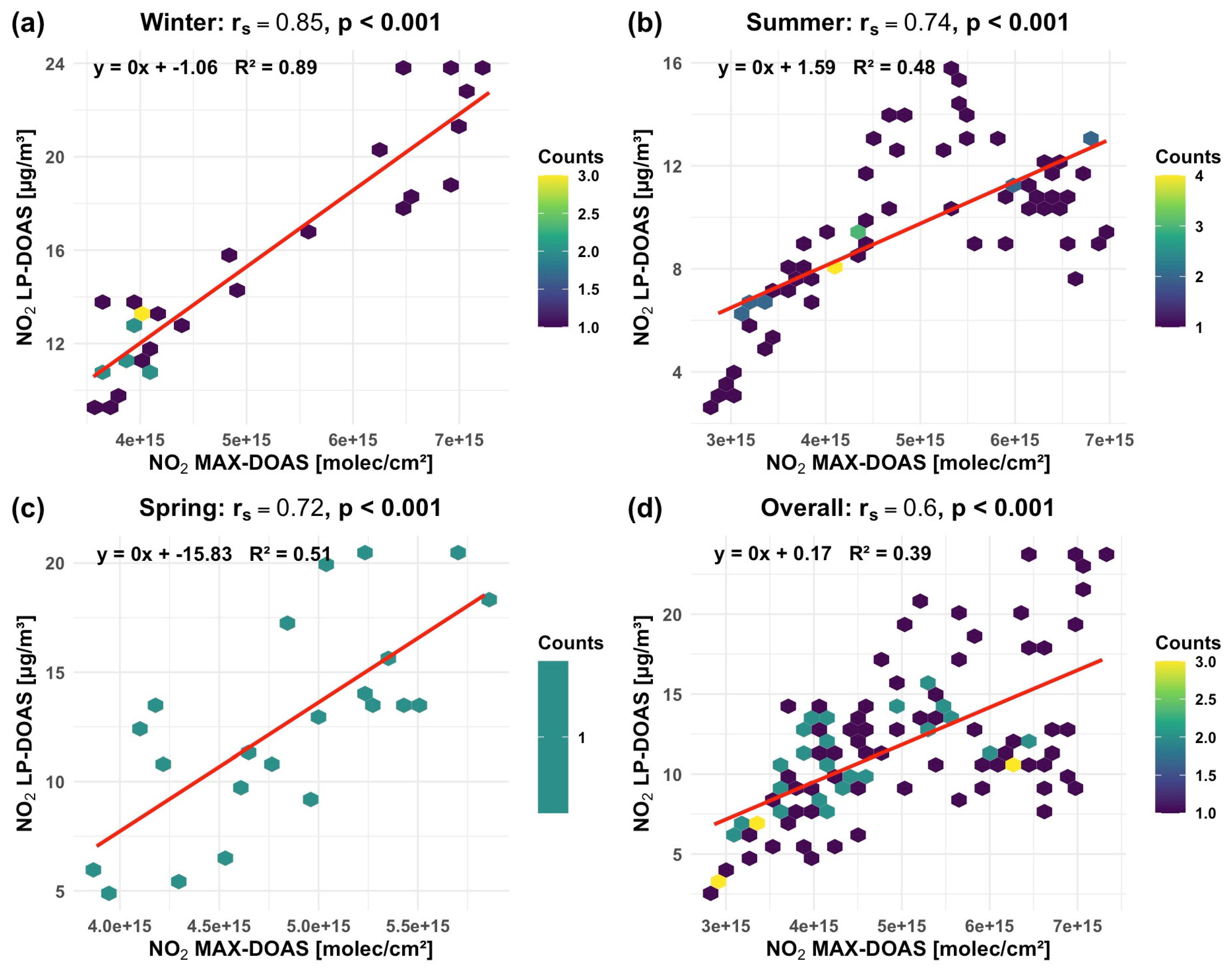
The normalisation of the NO₂ data was necessary to compare the relative variations between the two instruments, as MAX-DOAS measures slant column density in area units of cm⁻², while LP-DOAS provides volumetric measurements in volume units of cm⁻³. While normalisation allows for the identification of patterns, it also obscures the absolute differences in concentration levels. Figure 12 illustrates the seasonal variation in the correlation between NO₂ measurements obtained from MAX-DOAS and LP-DOAS. The strongest relationship is observed during winter (r_s = 0.85, R² = 0.89), indicating a high level of agreement between the two instruments under relatively stable atmospheric conditions, likely influenced by increased emissions and limited vertical mixing. In summer, the correlation decreases (r_s = 0.74, R² = 0.48), reflecting increased atmospheric dynamics, such as stronger photochemical activity and vertical mixing, which can dissociate column and near-surface NO₂ measurements.

Spring exhibits a comparable but slightly lower correlation (r_s = 0.72, R² = 0.51), representing transitional atmospheric conditions with moderate variability. The overall correlation (r_s = 0.60, R² = 0.39) is weaker due to the combined influence of seasonal variability. These results suggest that while both instruments capture similar NO₂ trends, differences in measurement sensitivity and atmospheric processes, particularly vertical distribution and mixing, contribute to variations in their agreement across seasons.

3.3. TROPOMI Measurements

3.3.1. Overview

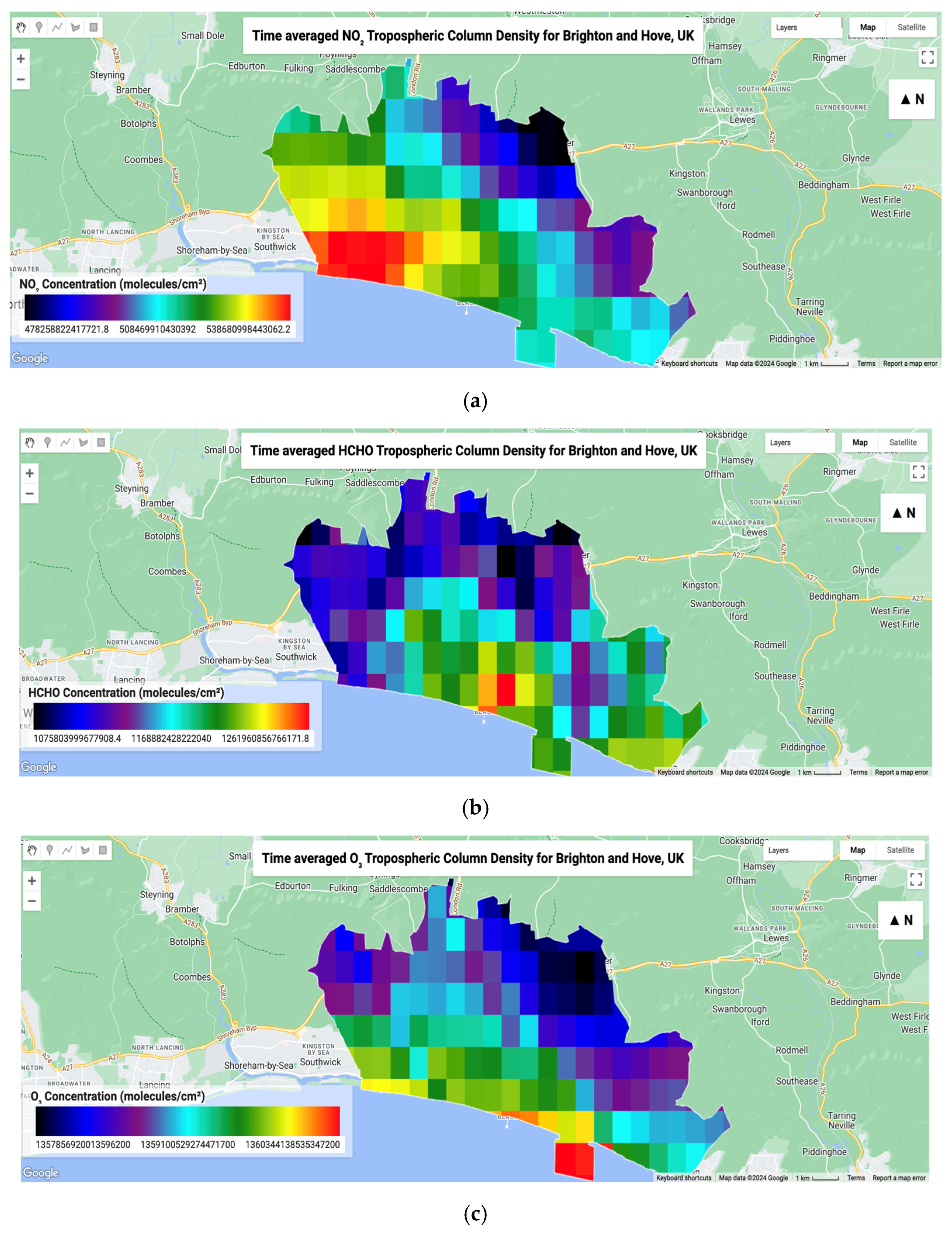
TROPOMI observations over Brighton and Hove County are presented in Figure 13. The figure reveals clear spatial variations in pollutant concentrations, with higher NO₂ concentrations in the southwestern part of the region, likely due to traffic and industrial emissions, while HCHO is more uniformly distributed, with a hotspot near the coast, indicating contributions from both anthropogenic and biogenic sources. Elevated ozone levels are also seen near the coast, potentially driven by sea breeze effects that transport precursor pollutants inland, leading to photochemical ozone formation.

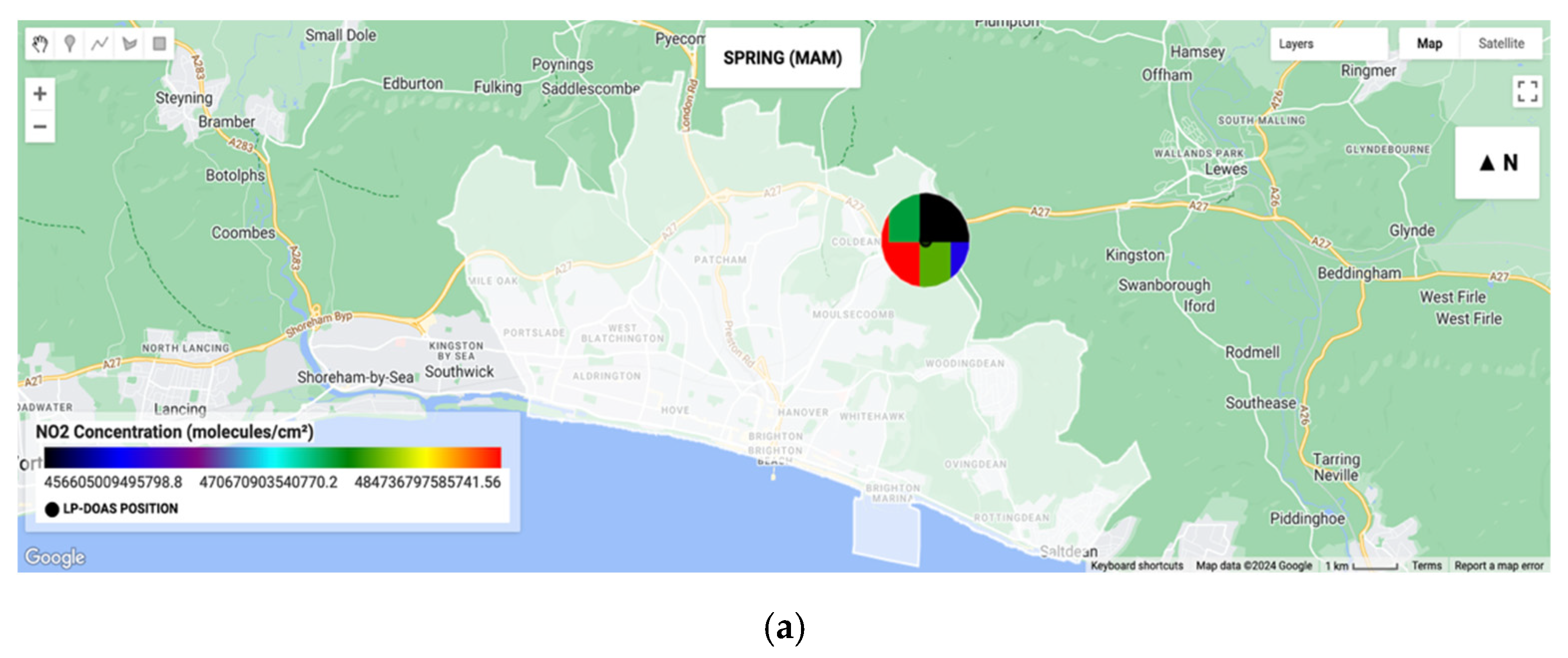
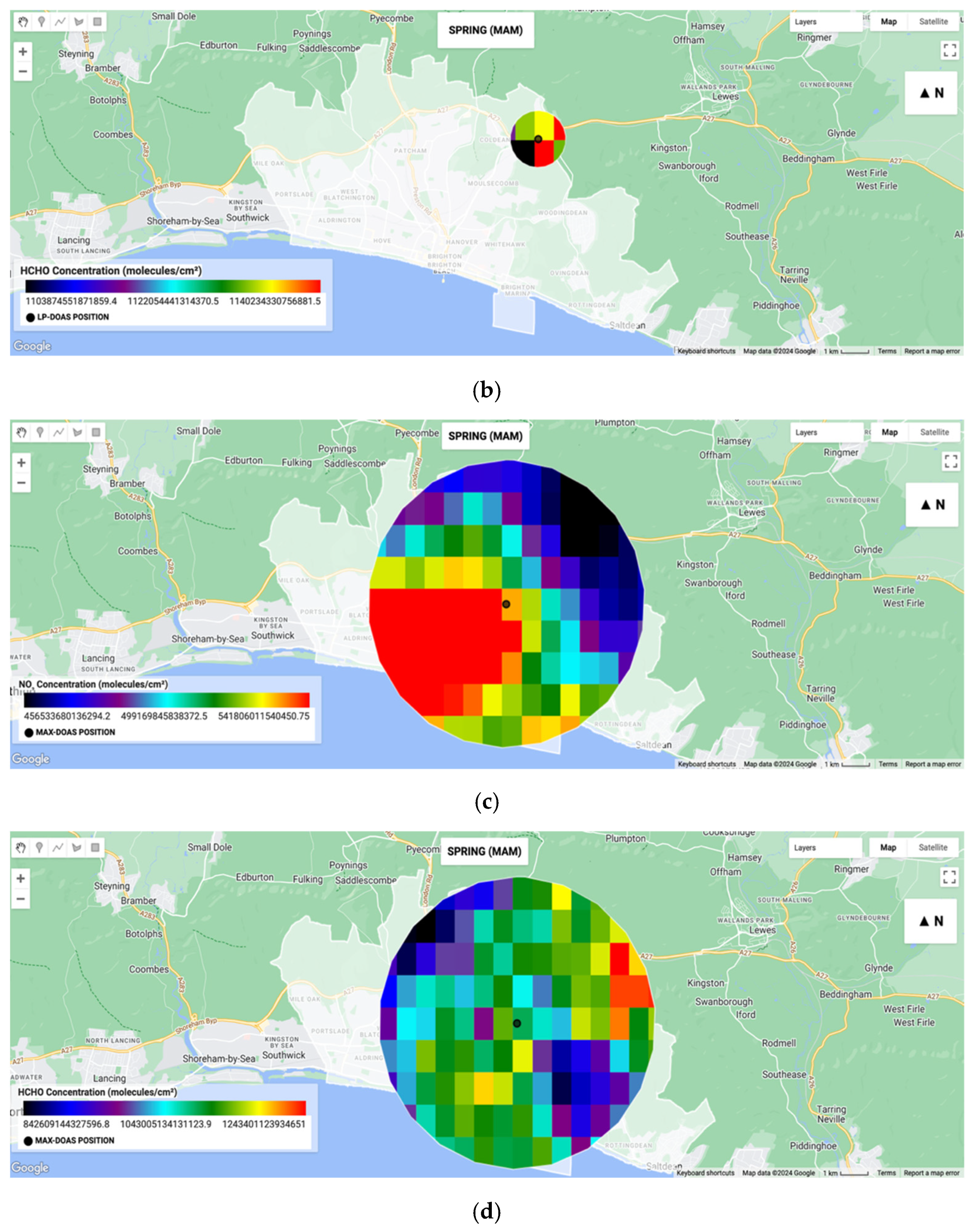
More detailed observations over the study sites in Brighton obtained from spatially and temporally averaged pixels are presented in

Table 5. Summary statistics for pollutant data measured by TROPOMI (molecules/cm²) for a 1 km buffer around the LP-DOAS (28/06/2018 to 01/06/2023) and a 5 km buffer around the MAX-DOAS (molecules/cm²) (01/07/2021 to 22/07/2021, 17/01/2022 to 05/09/2022, 20/03/2024 to 25/03/2024, and 16/05/2024 to 20/05/2024).

		LP-DOAS			MAX-DOAS
Season	Statistics	HCHO	NO2	O3	NO2
Spring	Mean	8.33 × 1014	4.63 × 1014	1.50 × 1018	4.50 × 1014
	Median	7.13 × 1014	4.30 × 1014	1.48 × 1018	4.34 × 1014
	St. dev.	6.24 × 1014	2.34 × 1014	1.30 × 1017	2.21 × 1014
	Min.	2.93 × 1012	4.95 × 1012	1.13 × 1018	2.52 × 1013
	Max.	3.41 × 1015	1.29 × 1015	1.94 × 1018	1.26 × 1015
Summer	Mean	1.07 × 1015	3.74 × 1014	1.36 × 1018	4.09 × 1014
	Median	9.28 × 1014	3.66 × 1014	1.34 × 1018	3.96 × 1014
	St. dev.	7.63 × 1014	1.68 × 1014	9.25 × 1016	1.66 × 1014
	Min.	1.77 × 1013	3.60 × 1013	1.17 × 1018	1.26 × 1014
	Max.	4.92 × 1015	1.25 × 1015	1.71 × 1018	9.15 × 1014
Autumn	Mean	9.59 × 1014	5.25 × 1014	1.22 × 1018
	Median	8.08 × 1014	4.72 × 1014	1.20 × 1018
	St. dev.	7.00 × 1014	2.69 × 1014	1.08 × 1017
	Min.	8.72 × 1012	4.49 × 1013	9.12 × 1017
	Max.	4.14 × 1015	1.89 × 1015	1.67 × 1018
Winter	Mean	1.02 × 1015	5.92 × 1014	1.33 × 1018	5.79 × 1014
	Median	8.47 × 1014	5.50 × 1014	1.31 × 1018	5.39 × 1014
	St. dev.	7.63 × 1014	3.39 × 1014	1.74 × 1017	3.34 × 1014
	Min.	5.41 × 1012	2.90 × 1013	9.22 × 1017	7.99 × 1013
	Max.	4.70 × 1015	1.92 × 1015	2.04 × 1018	2.11 × 1015
Annual	Mean	9.56 × 1014	4.82 × 1014	1.35 × 1018	4.74 × 1014
	Median	8.12 × 1014	4.37 × 1014	1.34 × 1018	4.45 × 1014
	St. dev.	7.09 × 1014	2.66 × 1014	1.66 × 1017	2.44 × 1014
	Min.	2.93 × 1012	4.95 × 1012	9.12 × 1017	2.52 × 1013
	Max.	4.92 × 1015	1.92 × 1015	2.04 × 1018	2.11 × 1015

and Figure 14. The circular heatmap overlays in the figures illustrate seasonal spatial variability and localised hotspots, while Table 5 quantifies these patterns. At the LP-DOAS site, NO₂ mean concentration values are lowest in summer (3.74 × 10¹⁴ molecules cm⁻²) and highest in winter (5.92 × 10¹⁴ molecules cm⁻²), reflecting increased emissions and reduced atmospheric mixing in colder months. In contrast, HCHO peaks in summer (1.07 × 10¹⁵ molecules cm⁻²) and remains relatively high in winter (1.02 × 10¹⁵ molecules cm⁻²), indicating the combined influence of photochemical production and seasonal emission sources. The large standard deviations and wide ranges between minimum and maximum values, particularly for HCHO, suggest substantial temporal variability and episodic enhancement.

At the MAX-DOAS site, NO₂ follows a similar seasonal trend, with higher concentrations in winter (5.79 × 10¹⁴ molecules cm⁻²) and lower values in summer (4.09 × 10¹⁴ molecules cm⁻²). However, compared to the LP-DOAS observations, the variability is reduced, reflecting the smoothing effect of the larger 5 km spatial averaging. Additionally, O₃ exhibits a spring maximum (1.50 × 10¹⁸ molecules cm⁻²), indicative of regional photochemical formation and transport.

3.3.2. Comparison with Ground-Based Measurements (LP-DOAS and MAX-DOAS)

TROPOMI vs. LP-DOAS

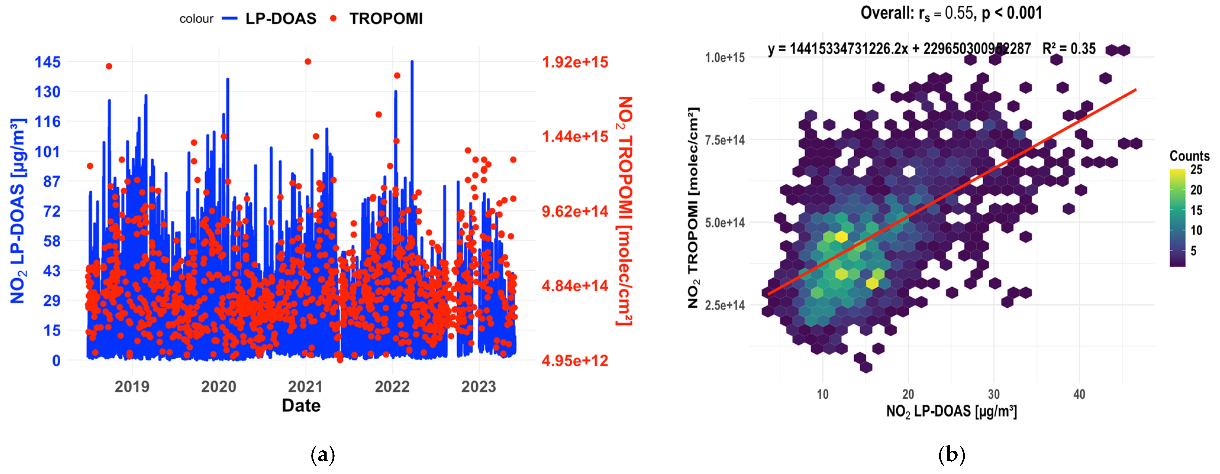
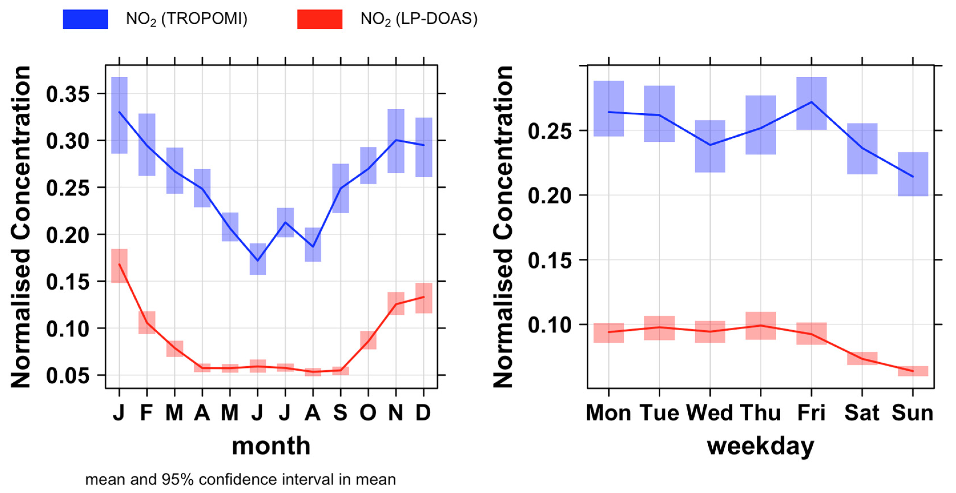
Figure 15a illustrates the concentration of NO₂ data measured by the LP-DOAS and TROPOMI for pixels within 1km (~3.14 km²) of LP-DOAS instruments. The LP-DOAS measurements are continuous and dense throughout the entire period, while TROPOMI data points are more sporadic, reflecting the satellite’s overpass frequency and the specific conditions required for data capture. Figure 16 shows a clear and similar monthly and weekday pattern for both instruments, with higher NO₂ levels during the colder months (November to February) and lower levels during the warmer months (June to September).

This pattern aligns with the typical behaviour of NO₂, where concentrations are generally higher in winter due to increased heating emissions and more stable atmospheric conditions.

The monthly trends captured by both instruments are consistent, although the difference in measurement scale is apparent. TROPOMI shows more significant monthly fluctuations, likely due to its ability to capture NO₂ over a broader area and in different atmospheric layers. Additionally, both instruments exhibit a similar weekly pattern, with higher NO₂ concentrations on weekdays and a noticeable decrease over the weekend, highlighting their capability to capture the impact of anthropogenic activities on NO₂ levels. The similarities between the instruments’ measurements are supported by the moderate positive correlation (r_s = 0.55) observed in Figure 15b.

The normalisation applied to these plots effectively highlights the relative changes in NO₂ concentrations over time. However, the difference in units makes it challenging to interpret the magnitude of concentration changes measured by both instruments. Direct conversion between these units would require additional assumptions regarding boundary layer height, vertical distribution of NO₂, and atmospheric mixing, which can introduce significant uncertainties.

TROPOMI vs. MAX-DOAS

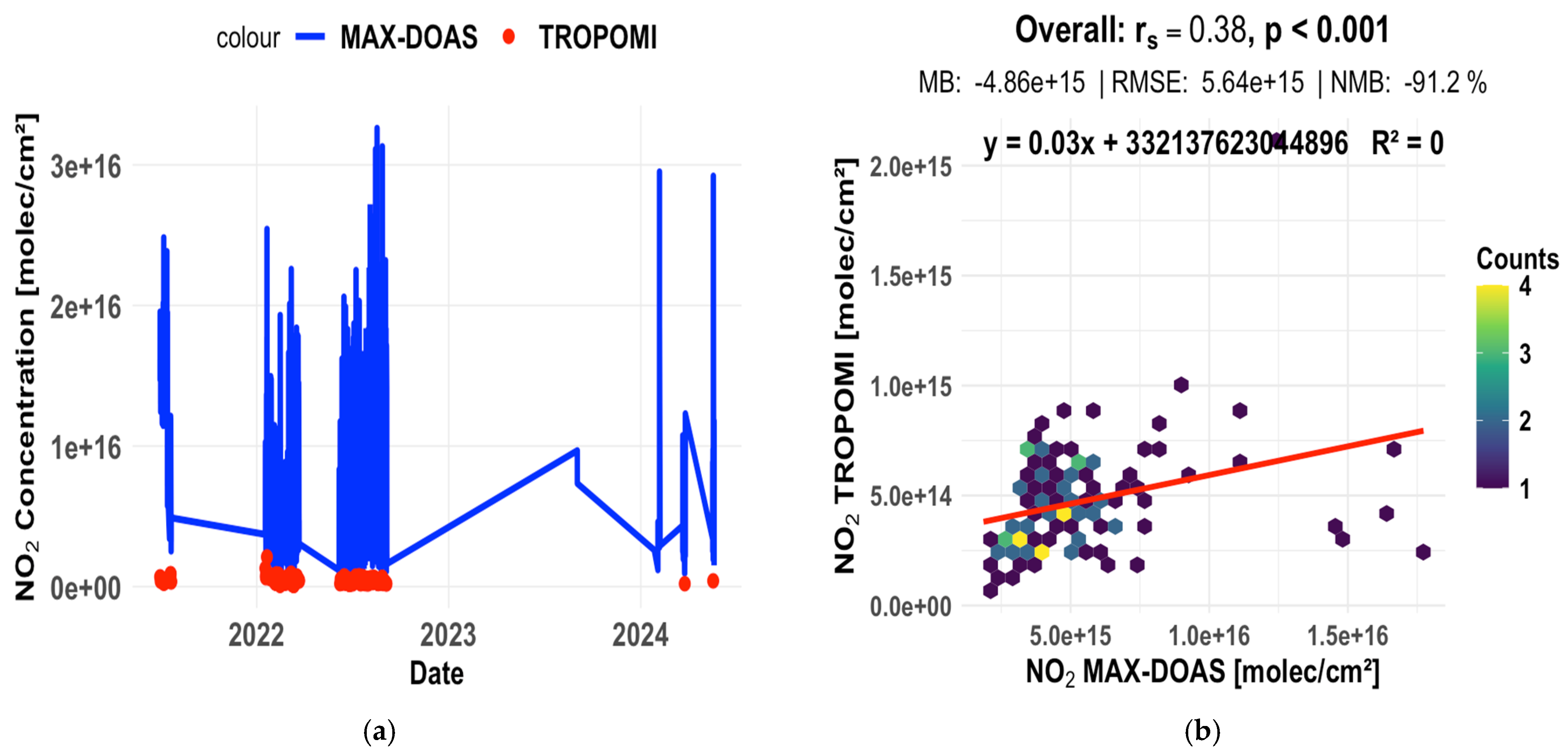
Figure 17a shows the time series of tropospheric NO₂ VCDs from MAX-DOAS and TROPOMI observations. The plot reveals significant differences in data density and concentration levels between the two instruments, highlighting the differences in their capabilities. Figure 17b illustrates a moderate positive correlation (r_s = 0.38) between the NO₂ measurements from MAX-DOAS and TROPOMI. This suggests that while the two instruments generally track NO₂ concentrations in the same direction, their measurements are not perfectly aligned. The negative mean bias (−4.86 × 10¹⁵) and high Root Mean Square Error (RMSE) (5.64 × 10¹⁵) indicate that TROPOMI underestimates NO₂ concentrations compared to MAX-DOAS, with substantial errors in measurement. This underestimation might be due to TROPOMI’s differences in vertical sensitivity, possibly being less responsive to NO₂ closer to the surface, where MAX-DOAS is more sensitive. Additionally, TROPOMI’s larger spatial averaging area could smooth out local concentration peaks captured by MAX-DOAS, leading to lower average concentrations, as suggested by other satellite studies [60,72,129]. The large negative Normalised Mean Bias (NMB) of −91.2% confirms the significant underestimation by TROPOMI, indicating that the bias is substantial not only in absolute terms but also relative to the overall NO₂ levels. Other studies have similarly documented TROPOMI’s underestimation of NO₂, partially attributing it to the coarse spatial a priori vertical distribution profile of NO₂ used in the AMF calculation during satellite retrievals in comparison to MAX-DOAS. Dimitropoulou et al. recorded an overall TROPOMI underestimation of MAX-DOAS by about 40–50% [73], while Chan et al. observed an average TROPOMI NO₂ underestimation of 30%, with MAX-DOAS NO₂ profiles showing approximately four times higher NO₂ levels at the surface compared to the original a priori profiles used in the satellite retrieval [71]. Studies have noted that using high-resolution and accurate a priori NO₂ profiles in TROPOMI retrievals could improve the accuracy of TROPOMI measurements [71,73,131,132].

4. Conclusions

This study represents a significant advancement in the understanding of urban air quality dynamics in Brighton, UK, through the integration of current and historical MAX-DOAS and Long-Path DOAS measurements with satellite data. The research successfully highlights the spatial and temporal distribution of key tropospheric pollutants (NO₂, SO₂, HCHO, O₃, and HONO), providing valuable insights into their seasonal and diurnal variations, sources, and the impact of urban infrastructure on their dispersion.

The results indicate significant seasonal and diurnal variations in pollutant concentrations, driven by factors such as traffic emissions, industrial activities, and weather patterns. Notably, the study emphasises the critical role of photochemical activity in the formation and degradation of secondary pollutants like HCHO and O₃, particularly during the summer months. The findings also underscore the persistent challenge of NO₂ pollution in Brighton, with traffic emissions being a dominant source, especially during rush hours and winter months.

The comparison between ground-based measurements and TROPOMI satellite data reveals both consistencies and discrepancies, with TROPOMI generally underestimating NO₂ levels compared to MAX-DOAS. This underestimation, while significant, highlights the need to refine the satellite retrieval algorithm by using MAX-DOAS NO₂ profiles as a priori information in the AMF calculation of the satellite retrieval to better capture near-surface pollution. The study also identifies limitations, particularly in the spatial resolution and sensitivity of satellite observations compared to ground-based measurements. The moderate positive correlations observed suggest that while satellite data provides valuable regional context, ground-based measurements remain essential for capturing local variations and ensuring the accuracy of air quality assessments.

This study contributes significantly to the field of urban atmospheric science by demonstrating the value of integrating diverse data sources for a more holistic understanding of air quality dynamics. The insights gained from this research are not only relevant to Brighton but can also inform air quality management strategies in other urban areas facing similar challenges.

Future research should focus on long-term monitoring to assess interannual variability and emission trends, while integrating additional observation platforms to improve satellite validation through multi-sensor data fusion. Furthermore, artificial intelligence (AI) and machine learning techniques could be explored to enhance satellite retrievals, predict pollutant distributions, and support more accurate urban air quality assessment and management.

References

1. Department for Environment, Food and Rural Affairs (DEFRA). Health Matters: Air Pollution. Available online: https://www.gov.uk/government/publications/health-matters-air-pollution/health-matters-air-pollution (accessed on 1 August 2024).
2. European Environment Agency (EEA). European Air Quality Status-2024. Available online: https://www.eea.europa.eu//publications/europes-air-quality-status-2024 (accessed on 1 August 2024).
3. Semlali, B.-E.B.; Amrani, C.E. A Stream Processing Software for Air Quality Satellite Datasets. In Advanced Intelligent Systems for Sustainable Development (AI2SD’2020); Springer International Publishing: Cham, Switzerland, 2022; pp. 839–853. [Google Scholar]
4. Bikis, A. Urban Air Pollution and Greenness in Relation to Public Health. J. Environ. Public Health 2023, 2023, 8516622. (In English) [Google Scholar] [CrossRef] [Scilit] [PubMed]
5. Liang, L.; Gong, P. Urban and air pollution: A multi-city study of long-term effects of urban landscape patterns on air quality trends. Sci. Rep. 2020, 10, 18618. [Google Scholar] [CrossRef] [Scilit] [PubMed]
6. WHO. Air Pollution. Available online: https://www.who.int/health-topics/air-pollution#tab=tab_1 (accessed on 20 April 2024).
7. Manisalidis, I.; Stavropoulou, E.; Stavropoulos, A.; Bezirtzoglou, E. Environmental and Health Impacts of Air Pollution: A Review. Front. Public Health 2020, 8, 14. (In English) [Google Scholar] [CrossRef] [Scilit] [PubMed]
8. Lee, B.J.; Kim, B.; Lee, K. Air pollution exposure and cardiovascular disease. Toxicol. Res. 2014, 30, 71–75. (In English) [Google Scholar] [CrossRef] [Scilit] [PubMed]
9. Brunekreef, B.; Holgate, S.T. Air pollution and health. Lancet (Br. Ed.) 2002, 360, 1233–1242. (In English) [Google Scholar] [CrossRef] [Scilit] [PubMed]
10. Lim, C.C.; Hayes, R.B.; Ahn, J.; Shao, Y.; Silverman, D.T.; Jones, R.R.; Garcia, C.; Thurston, G.D. Association between long-term exposure to ambient air pollution and diabetes mortality in the US. Environ. Res. 2018, 165, 330–336. (In English) [Google Scholar] [CrossRef] [Scilit] [PubMed]
11. Semlali, B.-E.B.; Amrani, C.E.; Ortiz, G.; Boubeta-Puig, J.; Garcia-de-Prado, A. SAT-CEP-monitor: An air quality monitoring software architecture combining complex event processing with satellite remote sensing. Comput. Electr. Eng. 2021, 93, 107257. [Google Scholar] [CrossRef] [Scilit]
12. Bell, J.N.B.; Power, S.A.; Jarraud, N.; Agrawal, M.; Davies, C. The effects of air pollution on urban ecosystems and agriculture. Int. J. Sustain. Dev. World Ecol. 2011, 18, 226–235. [Google Scholar] [CrossRef] [Scilit]
13. de Vries, W. Impacts of nitrogen emissions on ecosystems and human health: A mini review. Curr. Opin. Environ. Sci. Health 2021, 21, 100249. [Google Scholar] [CrossRef] [Scilit]
14. Matus, K.; Nam, K.-M.; Selin, N.E.; Lamsal, L.N.; Reilly, J.M.; Paltsev, S. Health damages from air pollution in China. Glob. Environ. Change 2012, 22, 55–66. [Google Scholar] [CrossRef] [Scilit]
15. Carozzi, F.; Roth, S. Dirty density: Air quality and the density of American cities. J. Environ. Econ. Manag. 2023, 118, 102767. [Google Scholar] [CrossRef] [Scilit]
16. Borck, R.; Schrauth, P. Population density and urban air quality. Reg. Sci. Urban Econ. 2021, 86, 103596. [Google Scholar] [CrossRef] [Scilit]
17. Nadadur, S.S.; Miller, C.A.; Hopke, P.K.; Gordon, T.; Vedal, S.; Vandenberg, J.J.; Costa, D.I. The complexities of air pollution regulation: The need for an integrated research and regulatory perspective. Toxicol. Sci. 2007, 100, 318–327. (In English) [Google Scholar] [CrossRef] [Scilit] [PubMed]
18. Sun, K.; Tao, L.; Miller, D.J.; Pan, D.; Golston, L.M.; Zondlo, M.A.; Griffin, R.J.; Wallace, H.W.; Leong, Y.J.; Yang, M.M.; et al. Vehicle Emissions as an Important Urban Ammonia Source in the United States and China. Environ. Sci. Technol. 2017, 51, 2472–2481. (In English) [Google Scholar] [CrossRef] [Scilit] [PubMed]
19. Li, S.; Liu, T.; Song, W.; Pei, C.; Huang, Z.; Wang, Y.; Chen, Y.; Yan, J.; Zhang, R.; Zhang, Y.; et al. Emission factors of ammonia for on-road vehicles in urban areas from a tunnel study in south China with laser-absorption based measurements. Environ. Pollut. 2021, 280, 116972. (In English) [Google Scholar] [CrossRef] [Scilit] [PubMed]
20. Rabia, M.; Muhammad, Z.; Ayesha, A.; Nadeem, Z.M. Industrial Air Emission Pollution: Potential Sources and Sustainable Mitigation. In Environmental Emissions; Richard, V., Ed.; IntechOpen: Rijeka, Croatia, 2021; Chapter 4. [Google Scholar]
21. Kjellstrom, T.; Lodh, M.; McMichael, T.; Ranmuthugala, G.; Shrestha, R.; Kingsland, S. Air and Water Pollution: Burden and Strategies for Control; International Bank for Reconstruction and Development/The World Bank: Washington, DC, USA, 2006. [Google Scholar]
22. Tomlin, A.S. Air Quality and Climate Impacts of Biomass Use as an Energy Source: A Review. Energy Fuels 2021, 35, 14213–14240. [Google Scholar] [CrossRef] [Scilit]
23. Chen, J.; Li, C.; Ristovski, Z.; Milic, A.; Gu, Y.; Islam, M.S.; Wang, S.; Hao, J.; Zhang, H.; He, C.; et al. A review of biomass burning: Emissions and impacts on air quality, health and climate in China. Sci. Total Environ. 2017, 579, 1000–1034. [Google Scholar] [CrossRef] [Scilit] [PubMed]
24. Shakhov, V.; Materukhin, A.; Sokolova, O.; Koo, I. Optimizing Urban Air Pollution Detection Systems. Sensors 2022, 22, 4767. [Google Scholar] [CrossRef] [Scilit] [PubMed]
25. Sahu, L. Volatile organic compounds and their measurements in the troposphere. Curr. Sci. 2012, 102, 1645–1649. [Google Scholar] [CrossRef] [Scilit]
26. Jacob, D.J.; Winner, D.A. Effect of climate change on air quality. Atmos. Environ. (1994) 2009, 43, 51–63. (In English) [Google Scholar] [CrossRef] [Scilit]
27. Ab Manan, N.; Noor Aizuddin, A.; Hod, R. Effect of Air Pollution and Hospital Admission: A Systematic Review. Ann. Glob. Health 2018, 84, 670–678. (In English) [Google Scholar] [CrossRef] [Scilit]
28. Grennfelt, P.; Engleryd, A.; Forsius, M.; Hov, Ø.; Rodhe, H.; Cowling, E. Acid rain and air pollution: 50 years of progress in environmental science and policy. Ambio 2020, 49, 849–864. [Google Scholar] [CrossRef] [Scilit] [PubMed]
29. WorldBank. The Global Health Cost of PM2.5 Air Pollution: A Case for Action Beyond 2021. In International Development in Focus; World Bank: Washington, DC, USA, 2022; Available online: http://hdl.handle.net/10986/36501 (accessed on 18 August 2024).
30. World Bank. Air Pollution Deaths Cost Global Economy US$225 Billion; World Bank: Washington, DC, USA, 2016. [Google Scholar]
31. Carslaw, D.; Farren, N.; Vaughan, A.; Drysdale, W.; Young, S.; Lee, J. The diminishing importance of nitrogen dioxide emissions from road vehicle exhaust. Atmos. Environ. X 2018, 1, 100002. [Google Scholar] [CrossRef] [Scilit]
32. Amato, F.; Cassee, F.R.; Denier van der Gon, H.A.C.; Gehrig, R.; Gustafsson, M.; Hafner, W.; Harrison, R.M.; Jozwicka, M.; Kelly, F.J.; Moreno, T.; et al. Urban air quality: The challenge of traffic non-exhaust emissions. J. Hazard. Mater. 2014, 275, 31–36. [Google Scholar] [CrossRef] [Scilit] [PubMed]
33. Monks, P.S.; Granier, C.; Fuzzi, S.; Stohl, A.; Williams, M.L.; Akimoto, H.; Amann, M.; Baklanov, A.; Baltensperger, U.; Bey, I.; et al. Atmospheric composition change—Global and regional air quality. Atmos. Environ. 2009, 43, 5268–5350. [Google Scholar] [CrossRef] [Scilit]
34. NAEI. Air Pollutant Inventories for England, Scotland, Wales and Northern Ireland: 2005–2021. Available online: https://uk-air.defra.gov.uk/assets/documents/reports/cat07/2310261138_DA_Air_Pollutant_Inventories_2005-2021_Final_v1.2.pdf (accessed on 23 August 2024).
35. Kleffmann, J. Daytime sources of nitrous acid (HONO) in the atmospheric boundary layer. ChemPhysChem 2007, 8, 1137–1144. (In English) [Google Scholar] [CrossRef] [Scilit] [PubMed]
36. Nurhisanah, S.; Hasyim, H. Environmental health risk assessment of sulfur dioxide (SO2) at workers around in combined cycle power plant (CCPP). Heliyon 2022, 8, e09388. (In English) [Google Scholar] [CrossRef] [Scilit] [PubMed]
37. Zhong, Q.; Shen, H.; Yun, X.; Chen, Y.; Ren, Y.A.; Xu, H.; Shen, G.; Meng, J.; Li, W.; Ma, J.; et al. Global Sulfur Dioxide Emissions and the Driving Forces. Environ. Sci. Technol. 2020, 54, 6508–6517. [Google Scholar] [CrossRef] [Scilit] [PubMed]
38. Benavent, N.; Garcia-Nieto, D.; Wang, S.; Saiz-Lopez, A. MAX-DOAS measurements and vertical profiles of glyoxal and formaldehyde in Madrid, Spain. Atmos. Environ. 2019, 199, 357–367. [Google Scholar] [CrossRef] [Scilit]
39. de Gouw, J.A.; Gilman, J.B.; Kim, S.W.; Alvarez, S.L.; Dusanter, S.; Graus, M.; Griffith, S.M.; Isaacman-VanWertz, G.; Kuster, W.C.; Lefer, B.L.; et al. Chemistry of Volatile Organic Compounds in the Los Angeles Basin: Formation of Oxygenated Compounds and Determination of Emission Ratios. J. Geophys. Res. Atmos. 2018, 123, 2298–2319. [Google Scholar] [CrossRef] [Scilit]
40. Kleffmann, J.; Gavriloaiei, T.; Hofzumahaus, A.; Holland, F.; Koppmann, R.; Rupp, L.; Schlosser, E.; Siese, M.; Wahner, A. Daytime formation of nitrous acid: A major source of OH radicals in a forest. Geophys. Res. Lett.-Geophys. Res. Lett. 2005, 32, L05818. [Google Scholar] [CrossRef] [Scilit]
41. Guo, S.; Chen, M.; Tan, J. Seasonal and diurnal characteristics of atmospheric carbonyls in Nanning, China. Atmos. Res. 2016, 169, 46–53. [Google Scholar] [CrossRef] [Scilit]
42. Monks, P.S.; Archibald, A.T.; Colette, A.; Cooper, O.; Coyle, M.; Derwent, R.; Fowler, D.; Granier, C.; Law, K.S.; Mills, G.E.; et al. Tropospheric ozone and its precursors from the urban to the global scale from air quality to short-lived climate forcer. Atmos. Chem. Phys. 2015, 15, 8889–8973. [Google Scholar] [CrossRef] [Scilit]
43. BHCC. Brighton & Hove City Council; 2024 Air Quality Annual Status Report (ASR). Available online: https://www.brighton-hove.gov.uk/sites/default/files/2024-07/ASR_Brighton%20%26%20Hove_2024%20V2.asd_.pdf (accessed on 3 August 2024).
44. Department for Environment, Food and Rural Affairs (DEFRA). National List and Despription of Air Quality Management Areas (Brighton and Hove Council). Available online: https://uk-air.defra.gov.uk/aqma/local-authorities?la_id=35 (accessed on 14 May 2024).
45. Snyder, E.G.; Watkins, T.H.; Solomon, P.A.; Thoma, E.D.; Williams, R.W.; Hagler, G.S.W.; Shelow, D.; Hindin, D.A.; Kilaru, V.J.; Preuss, P.W. The Changing Paradigm of Air Pollution Monitoring. Environ. Sci. Technol. 2013, 47, 11369–11377. [Google Scholar] [CrossRef] [Scilit] [PubMed]
46. Zheng, X.; Javed, Z.; Liu, C.; Tanvir, A.; Sandhu, O.; Liu, H.; Ji, X.; Xing, C.; Lin, H.; Du, D. MAX-DOAS and in-situ measurements of aerosols and trace gases over Dongying, China: Insight into ozone formation sensitivity based on secondary HCHO. J. Environ. Sci. 2024, 135, 656–668. [Google Scholar] [CrossRef] [Scilit] [PubMed]
47. Wang, H.; Wei, W.; Che, H.; Tang, X.; Bian, J.; Yu, K.; Wang, W. Ground-Based MAX-DOAS Measurements of Tropospheric Aerosols, NO2, and HCHO Distributions in the Urban Environment of Shanghai, China. Remote Sens. 2022, 14, 1726. [Google Scholar] [CrossRef] [Scilit]
48. Wang, Y.; Apituley, A.; Bais, A.; Beirle, S.; Benavent, N.; Borovski, A.; Bruchkouski, I.; Chan, K.L.; Donner, S.; Drosoglou, T.; et al. Inter-comparison of MAX-DOAS measurements of tropospheric HONO slant column densities and vertical profiles during the CINDI-2 campaign. Atmos. Meas. Tech. 2020, 13, 5087–5116. [Google Scholar] [CrossRef] [Scilit]
49. Lauster, B.; Dörner, S.; Beirle, S.; Donner, S.; Gromov, S.; Uhlmannsiek, K.; Wagner, T. Estimating real driving emissions from multi-axis differential optical absorption spectroscopy (MAX-DOAS) measurements at the A60 motorway near Mainz, Germany. Atmos. Meas. Tech. 2021, 14, 769–783. [Google Scholar] [CrossRef] [Scilit]
50. Hoque, H.M.S.; Sudo, K.; Irie, H.; Damiani, A.; Naja, M.; Fatmi, A.M. Multi-axis differential optical absorption spectroscopy (MAX-DOAS) observations of formaldehyde and nitrogen dioxide at three sites in Asia and comparison with the global chemistry transport model CHASER. Atmos. Chem. Phys. 2022, 22, 12559–12589. [Google Scholar] [CrossRef] [Scilit]
51. Wang, Y.; Dörner, S.; Donner, S.; Böhnke, S.; De Smedt, I.; Dickerson, R.R.; Dong, Z.; He, H.; Li, Z.; Li, D.; et al. Vertical profiles of NO2, SO2, HONO, HCHO, CHOCHO and aerosols derived from MAX-DOAS measurements at a rural site in the central western North China Plain and their relation to emission sources and effects of regional transport. Atmos. Chem. Phys. 2019, 19, 5417–5449. [Google Scholar] [CrossRef] [Scilit]
52. Li, X.; Brauers, T.; Shao, M.; Garland, R.M.; Wagner, T.; Deutschmann, T.; Wahner, A. MAX-DOAS measurements in southern China: Retrieval of aerosol extinctions and validation using ground-based in-situ data. Atmos. Chem. Phys. 2010, 10, 2079–2089. [Google Scholar] [CrossRef] [Scilit]
53. Ma, J.Z.; Beirle, S.; Jin, J.L.; Shaiganfar, R.; Yan, P.; Wagner, T. Tropospheric NO2 vertical column densities over Beijing: Results of the first three years of ground-based MAX-DOAS measurements (2008–2011) and satellite validation. Atmos. Chem. Phys. 2013, 13, 1547–1567. [Google Scholar] [CrossRef] [Scilit]
54. Kang, Y.; Tang, G.; Li, Q.; Liu, B.; Cao, J.; Hu, Q.; Wang, Y. Evaluation and Evolution of MAX-DOAS-observed Vertical NO2 Profiles in Urban Beijing. Adv. Atmos. Sci. 2021, 38, 1188–1196. [Google Scholar] [CrossRef] [Scilit]
55. Ryan, R.G.; Marais, E.A.; Gershenson-Smith, E.; Ramsay, R.; Muller, J.P.; Tirpitz, J.L.; Frieß, U. Measurement report: MAX-DOAS measurements characterise Central London ozone pollution episodes during 2022 heatwaves. Atmos. Chem. Phys. 2023, 23, 7121–7139. [Google Scholar] [CrossRef] [Scilit]
56. Hendrick, F.; Müller, J.F.; Clémer, K.; Wang, P.; De Mazière, M.; Fayt, C.; Gielen, C.; Hermans, C.; Ma, J.Z.; Pinardi, G.; et al. Four years of ground-based MAX-DOAS observations of HONO and NO2 in the Beijing area. Atmos. Chem. Phys. 2014, 14, 765–781. [Google Scholar] [CrossRef] [Scilit]
57. Yu, Y.; Galle, B.; Panday, A.; Hodson, E.; Prinn, R.; Wang, S. Observations of high rates of NO2-HONO conversion in the nocturnal atmospheric boundary layer in Kathmandu, Nepal. Atmos. Chem. Phys. 2009, 9, 6401–6415. [Google Scholar] [CrossRef] [Scilit]
58. Zheng, N.; Chan, K.L.; Xie, P.; Qin, M.; Ling, L.; Wu, F.; Hu, R. Observations of atmospheric trace gases in China using a compact LED long path DOAS system. Atmos. Pollut. Res. 2018, 9, 379–387. [Google Scholar] [CrossRef] [Scilit]
59. Lu, X.; Qin, M.; Xie, P.; Duan, J.; Fang, W.; Shen, L.; Liu, J.; Liu, W. Observation of NO3 Radicals by LP-DOAS over Hefei, China; Optica Publishing Group: Washington, DC, USA, 2015. [Google Scholar]
60. Chan, K.L.; Pöhler, D.; Kuhlmann, G.; Hartl, A.; Platt, U.; Wenig, M.O. NO2 measurements in Hong Kong using LED based long path differential optical absorption spectroscopy. Atmos. Meas. Tech. 2012, 5, 901–912. [Google Scholar] [CrossRef] [Scilit]
61. Asaf, D.; Tas, E.; Pedersen, D.; Peleg, M.; Luria, M. Long-Term Measurements of NO3 Radical at a Semiarid Urban Site: 2. Seasonal Trends and Loss Mechanisms. Environ. Sci. Technol. 2010, 44, 5901–5907. [Google Scholar] [CrossRef] [Scilit] [PubMed]
62. Volkamer, R.; Molina, L.T.; Molina, M.J.; Shirley, T.; Brune, W.H. DOAS measurement of glyoxal as an indicator for fast VOC chemistry in urban air. Geophys. Res. Lett. 2005, 32, L08806. [Google Scholar] [CrossRef] [Scilit]
63. Wang, S.; Ackermann, R.; Stutz, J. Vertical profiles of O3 and NOx chemistry in the polluted nocturnal boundary layer in Phoenix, AZ: I. Field observations by long-path DOAS. Atmos. Chem. Phys. 2006, 6, 2671–2693. [Google Scholar] [CrossRef] [Scilit]
64. Stutz, J.; Alicke, B.; Ackermann, R.; Geyer, A.; Wang, S.; White, A.B.; Williams, E.J.; Spicer, C.W.; Fast, J.D. Relative humidity dependence of HONO chemistry in urban areas. J. Geophys. Res. Atmos. 2004, 109. [Google Scholar] [CrossRef] [Scilit]
65. Veitel, H.; Kromer, B.; Mossner, M.; Platt, U. New techniques for measurements of atmospheric vertical trace gas profiles using DOAS. Environ. Sci. Pollut. Res. 2002, 9, 17–26. [Google Scholar]
66. Garcia-Nieto, D.; Benavent, N.; Borge, R.; Saiz-Lopez, A. Two-dimensional monitoring of air pollution in Madrid using a Multi-AXis Differential Optical Absorption Spectroscopy two-dimensional (MAXDOAS-2D) instrument. Atmos. Meas. Tech. 2021, 14, 2941–2955. [Google Scholar] [CrossRef] [Scilit]
67. Frieß, U.; Monks, P.S.; Remedios, J.J.; Rozanov, A.; Sinreich, R.; Wagner, T.; Platt, U. MAX-DOAS O4 measurements: A new technique to derive information on atmospheric aerosols: 2. Modeling studies. J. Geophys. Res. Atmos. 2006, 111, D14203. [Google Scholar] [CrossRef] [Scilit]
68. Johnson, J.B. An Introduction to Atmospheric Pollutant Dispersion Modelling. Environ. Sci. Proc. 2022, 19, 18. [Google Scholar] [CrossRef] [Scilit]
69. Liu, B.; Wu, C.; Ma, N.; Chen, Q.; Li, Y.; Ye, J.; Martin, S.T.; Li, Y.J. Vertical profiling of fine particulate matter and black carbon by using unmanned aerial vehicle in Macau, China. Sci. Total Environ. 2020, 709, 136109. [Google Scholar] [CrossRef] [Scilit] [PubMed]
70. Zhou, B.; Zhang, S.; Xue, R.; Li, J.; Wang, S. A review of Space-Air-Ground integrated remote sensing techniques for atmospheric monitoring. J. Environ. Sci. 2023, 123, 3–14. [Google Scholar] [CrossRef] [Scilit] [PubMed]
71. Chan, K.L.; Wiegner, M.; van Geffen, J.; De Smedt, I.; Alberti, C.; Cheng, Z.; Ye, S.; Wenig, M. MAX-DOAS measurements of tropospheric NO2 and HCHO in Munich and the comparison to OMI and TROPOMI satellite observations. Atmos. Meas. Tech. 2020, 13, 4499–4520. [Google Scholar] [CrossRef] [Scilit]
72. Chong, J.; Kim, Y.J.; Gu, M.; Wagner, T.; Song, C.H. Mobile MAX-DOAS observation of NO2 and comparison with OMI satellite data in the western coastal areas of the Korean peninsula. Chemosphere 2016, 143, 10–16. (In English) [Google Scholar] [CrossRef] [Scilit] [PubMed]
73. Dimitropoulou, E.; Hendrick, F.; Pinardi, G.; Friedrich, M.M.; Merlaud, A.; Tack, F.; De Longueville, H.; Fayt, C.; Hermans, C.; Laffineur, Q.; et al. Validation of TROPOMI tropospheric NO2 columns using dual-scan multi-axis differential optical absorption spectroscopy (MAX-DOAS) measurements in Uccle, Brussels. Atmos. Meas. Tech. 2020, 13, 5165–5191. [Google Scholar] [CrossRef] [Scilit]
74. Shoaib, A.; Khokhar, M.F.; Sandhu, O. Investigating the temporal variation of formaldehyde using MAX-DOAS and satellite observations over Islamabad, Pakistan. Atmos. Pollut. Res. 2020, 11, 193–204. [Google Scholar] [CrossRef] [Scilit]
75. Jin, J.; Ma, J.; Lin, W.; Zhao, H.; Shaiganfar, R.; Beirle, S.; Wagner, T. MAX-DOAS measurements and satellite validation of tropospheric NO2 and SO2 vertical column densities at a rural site of North China. Atmos. Environ. 2016, 133, 12–25. [Google Scholar] [CrossRef] [Scilit]
76. Stutz, J.; Thomas, J.L.; Hurlock, S.C.; Schneider, M.; von Glasow, R.; Piot, M.; Gorham, K.; Burkhart, J.F.; Ziemba, L.; Dibb, J.E.; et al. Longpath DOAS observations of surface BrO at Summit, Greenland. Atmos. Chem. Phys. 2011, 11, 9899–9910. [Google Scholar] [CrossRef] [Scilit]
77. Hönninger, G.; von Friedeburg, C.; Platt, U. Multi-axis differential optical absorption spectroscopy (MAX-DOAS). Atmos. Chem. Phys. 2004, 4, 231–254. [Google Scholar] [CrossRef] [Scilit]
78. Platt, U.; Stutz, J. Differential Optical Absorption Spectroscopy (DOAS)—Principles and Applications; Springer: Berlin/Heidelberg, Germany, 2008. [Google Scholar]
79. Platt, U. Air Monitoring by Differential Optical Absorption Spectroscopy. In Encyclopedia of Analytical Chemistry; Wiley: Hoboken, NJ, USA, 2017; pp. 1–28. [Google Scholar]
80. Vandaele, A.C.; Hermans, C.; Simon, P.; Carleer, M.; Colin, R.; Fally, S.; Mérienne, M.F.; Jenouvrier, A.; Coquart, B. Measurements of the NO2 absorption cross-section from 42,000 cm−1 to 10,000 cm−1 (238–1000 nm) at 220 K and 294 K. J. Quant. Spectrosc. Radiat. Transf. 1998, 59, 171–184. [Google Scholar] [CrossRef] [Scilit]
81. Bogumil, K.; Orphal, J.; Homann, T.; Voigt, S.; Spietz, P.; Fleischmann, O.C.; Vogel, A.; Hartmann, M.; Kromminga, H.; Bovensmann, H.; et al. Measurements of molecular absorption spectra with the SCIAMACHY pre-flight model: Instrument characterization and reference data for atmospheric remote-sensing in the 230–2380 nm region. J. Photochem. Photobiol. A Chem. 2003, 157, 167–184. [Google Scholar] [CrossRef] [Scilit]
82. Vandaele, A.C.; Hermans, C.; Fally, S. Fourier transform measurements of SO2 absorption cross sections: II. Temperature dependence in the 29,000-44,000 cm−1 (227–345 nm) region. J. Quant. Spectrosc. Radiat. Transf. 2009, v110, 2115–2126. [Google Scholar] [CrossRef] [Scilit]
83. Serdyuchenko, A.; Gorshelev, V.; Weber, M.; Chehade, W.; Burrows, J.P. High spectral resolution ozone absorption cross-sections—Part 2: Temperature dependence. Atmos. Meas. Tech. 2014, 7, 625–636. [Google Scholar] [CrossRef] [Scilit]
84. Fleischmann, O.C.; Hartmann, M.; Burrows, J.P.; Orphal, J. New ultraviolet absorption cross-sections of BrO at atmospheric temperatures measured by time-windowing Fourier transform spectroscopy. J. Photochem. Photobiol. A Chem. 2004, 168, 117–132. [Google Scholar] [CrossRef] [Scilit]
85. Chance, K.; Orphal, J. Revised ultraviolet absorption cross sections of H2CO for the HITRAN database. J. Quant. Spectrosc. Radiat. Transf. 2011, 112, 1509–1510. [Google Scholar] [CrossRef] [Scilit]
86. Stutz, J.; Kim, E.S.; Platt, U.; Bruno, P.; Perrino, C.; Febo, A. UV-visible absorption cross sections of nitrous acid. J. Geophys. Res. Atmos. 2000, 105, 14585–14592. [Google Scholar] [CrossRef] [Scilit]
87. Volkamer, R.; Spietz, P.; Burrows, J.; Platt, U. High-resolution absorption cross-section of Glyoxal in the UV/VIS and IR spectral ranges. J. Photochem. Photobiol. A Chem. 2005, 172, 35–46. [Google Scholar] [CrossRef] [Scilit]
88. Nasse, J.M.; Eger, P.G.; Pöhler, D.; Schmitt, S.; Frieß, U.; Platt, U. Recent improvements of long-path DOAS measurements: Impact on accuracy and stability of short-term and automated long-term observations. Atmos. Meas. Tech. 2019, 12, 4149–4169. [Google Scholar] [CrossRef] [Scilit]
89. Brighton Atmospheric Observatory (BAO). Available online: https://www.brighton.ac.uk/business-services/collaborate/climate-change/natural-resources.aspx (accessed on 5 June 2024).
90. Veefkind, J.P.; Aben, I.; McMullan, K.; Förster, H.; de Vries, J.; Otter, G.; Claas, J.; Eskes, H.J.; de Haan, J.F.; Kleipool, M. TROPOMI on the ESA Sentinel-5 Precursor: A GMES Mission for Global Observations of the Atmospheric Composition for Climate, Air Quality and Ozone Layer Applications. Remote Sens. Environ. 2012, 120, 70. [Google Scholar] [CrossRef] [Scilit]
91. Douros, J.; Eskes, H.; van Geffen, J.; Boersma, K.F.; Compernolle, S.; Pinardi, G.; Blechschmidt, A.M.; Peuch, V.H.; Colette, A.; Veefkind, P. Comparing Sentinel-5P TROPOMI NO2 column observations with the CAMS regional air quality ensemble. Geosci. Model Dev. 2023, 16, 509–534. [Google Scholar] [CrossRef] [Scilit]
92. Goldberg, D.L.; Lu, Z.; Streets, D.G.; de Foy, B.; Griffin, D.; McLinden, C.A.; Lamsal, L.N.; Krotkov, N.A.; Eskes, H. Enhanced Capabilities of TROPOMI NO2: Estimating NOX from North American Cities and Power Plants. Environ. Sci. Technol. 2019, 53, 12594–12601. [Google Scholar] [CrossRef] [Scilit] [PubMed]
93. Miyazaki, K.; Bowman, K.; Sekiya, T.; Jiang, Z.; Chen, X.; Eskes, H.; Ru, M.; Zhang, Y.; Shindell, D. Air Quality Response in China Linked to the 2019 Novel Coronavirus (COVID-19) Lockdown. Geophys. Res. Lett. 2020, 47, e2020GL089252. [Google Scholar] [CrossRef] [Scilit] [PubMed]
94. Georgoulias, A.K.; Boersma, K.F.; van Vliet, J.; Zhang, X.; van der A, R.; Zanis, P.; de Laat, J. Detection of NO2 pollution plumes from individual ships with the TROPOMI/S5P satellite sensor. Environ. Res. Lett. 2020, 15, 124037. [Google Scholar] [CrossRef] [Scilit]
95. DEFRA. Air Quality Statistics in the UK, 1987 to 2023—Nitrogen Dioxide (NO2). Available online: https://www.gov.uk/government/statistics/air-quality-statistics/ntrogen-dioxide#:~:text=The%20Air%20Quality%20Standards%20Regulations,3)%20in%20a%20single%20year. (accessed on 30 August 2024).
96. DEFRA. Nitrogen Dioxide in the United Kingdom. Available online: https://uk-air.defra.gov.uk/library/assets/documents/reports/aqeg/nitrogen_dioxide_in_the_UK-summary.pdf (accessed on 30 August 2024).
97. DEFRA. Air Quality Statistics in the UK, 1987 to 2023—Ozone (O3). Available online: https://www.gov.uk/government/statistics/air-quality-statistics/concentrations-of-ozone (accessed on 30 August 2024).
98. Niepsch, D.; Clarke, L.J.; Tzoulas, K.; Cavan, G. Spatiotemporal variability of nitrogen dioxide (NO2) pollution in Manchester (UK) city centre (2017–2018) using a fine spatial scale single-NOx diffusion tube network. Environ. Geochem. Health 2022, 44, 3907–3927. [Google Scholar] [CrossRef] [Scilit] [PubMed]
99. Kirby, C.; Greig, A.; Drye, T. Temporal and spatial variations in nitrogen dioxide concentrations across an urban landscape: Cambridge, UK. Environ. Monit. Assess. 1998, 52, 65–82. (In English) [Google Scholar] [CrossRef] [Scilit]
100. Bower, J.S.; Broughton, G.; Dando, M.; Lees, A.; Stevenson, K.; Lampert, J.; Sweeney, B.; Parker, V.; Driver, G.; Waddon, C.; et al. Urban NO2 concentrations in the U.K. in 1987, Atmospheric Environment. Part B Urban Atmos. 1991, 25, 267–283. [Google Scholar] [CrossRef] [Scilit]
101. Wyche, K.P.; Nichols, M.; Parfitt, H.; Beckett, P.; Gregg, D.J.; Smallbone, K.L.; Monks, P.S. Changes in ambient air quality and atmospheric composition and reactivity in the South East of the UK as a result of the COVID-19 lockdown. Sci. Total Environ. 2021, 755, 142526. [Google Scholar] [CrossRef] [Scilit] [PubMed]
102. Makra, L.; Mayer, H.; Mika, J.; Sánta, T.; Holst, J. Variations of traffic related air pollution on different time scales in Szeged, Hungary and Freiburg, Germany. Phys. Chem. Earth Parts A/B/C 2010, 35, 85–94. [Google Scholar] [CrossRef] [Scilit]
103. Indarto, A. Heterogeneous reactions of HONO formation from NO2 and HNO3: A review. Res. Chem. Intermed. 2012, 38, 1029–1041. [Google Scholar] [CrossRef] [Scilit]
104. Kurtenbach, R.; Becker, K.H.; Gomes, J.A.G.; Kleffmann, J.; Lörzer, J.C.; Spittler, M.; Wiesen, P.; Ackermann, R.; Geyer, A.; Platt, U. Investigations of emissions and heterogeneous formation of HONO in a road traffic tunnel. Atmos. Environ. 2001, 35, 3385–3394. [Google Scholar] [CrossRef] [Scilit]
105. Gratsea, M.; Vrekoussis, M.; Richter, A.; Wittrock, F.; Schönhardt, A.; Burrows, J.; Kazadzis, S.; Mihalopoulos, N.; Gerasopoulos, E. Slant column MAX-DOAS measurements of nitrogen dioxide, formaldehyde, glyoxal and oxygen dimer in the urban environment of Athens. Atmos. Environ. 2016, 135, 118–131. [Google Scholar] [CrossRef] [Scilit]
106. Fortems-Cheiney, A.; Chevallier, F.; Pison, I.; Bousquet, P.; Saunois, M.; Szopa, S.; Cressot, C.; Kurosu, T.P.; Chance, K.; Fried, A. The formaldehyde budget as seen by a global-scale multi-constraint and multi-species inversion system. Atmos. Chem. Phys. 2012, 12, 6699–6721. [Google Scholar] [CrossRef] [Scilit]
107. De Smedt, I.; Müller, J.F.; Stavrakou, T.; van der A, R.; Eskes, H.; Van Roozendael, M. Twelve years of global observations of formaldehyde in the troposphere using GOME and SCIAMACHY sensors. Atmos. Chem. Phys. 2008, 8, 4947–4963. [Google Scholar] [CrossRef] [Scilit]
108. Atkinson, R.W.; Yu, D.; Armstrong, B.G.; Pattenden, S.; Wilkinson, P.; Doherty, R.M.; Heal, M.R.; Anderson, H.R. Concentration-response function for ozone and daily mortality: Results from five urban and five rural U.K. populations. Environ. Health Perspect. 2012, 120, 1411–1417. (In English) [Google Scholar] [CrossRef] [Scilit] [PubMed]
109. Jenkin, M. Analysis of sources and partitioning of oxidant in the UK—Part 1: The NO X-dependence of annual mean concentrations of nitrogen dioxide and ozone. Atmos. Environ. 2004, 38, 5117–5129. [Google Scholar] [CrossRef] [Scilit]
110. Jenkin, M.E. Trends in ozone concentration distributions in the UK since 1990: Local, regional and global influences. Atmos. Environ. 2008, 42, 5434–5445. [Google Scholar] [CrossRef] [Scilit]
111. Dueñas, C.; Fernández, M.C.; Cañete, S.; Carretero, J.; Liger, E. Assessment of ozone variations and meteorological effects in an urban area in the Mediterranean Coast. Sci. Total Environ. 2002, 299, 97–113. (In English) [Google Scholar] [CrossRef] [Scilit] [PubMed]
112. Valach, A.C.; Langford, B.; Nemitz, E.; MacKenzie, A.R.; Hewitt, C.N. Seasonal and diurnal trends in concentrations and fluxes of volatile organic compounds in central London. Atmos. Chem. Phys. 2015, 15, 7777–7796. [Google Scholar] [CrossRef] [Scilit]
113. Song, F.; Young Shin, J.; Jusino-Atresino, R.; Gao, Y. Relationships among the springtime ground–level NOx, O3 and NO3 in the vicinity of highways in the US East Coast. Atmos. Pollut. Res. 2011, 2, 374–383. [Google Scholar] [CrossRef] [Scilit]
114. Matthaios, V.; Kramer, L.; Sommariva, R.; Pope, F.; Bloss, W. Investigation of vehicle cold start primary NO2 emissions from ambient monitoring data in the UK and their implications for urban air quality. Atmos. Environ. 2018, 199, 402–414. [Google Scholar] [CrossRef] [Scilit]
115. Fantozzi, F.; Monaci, F.; Blanusa, T.; Bargagli, R. Spatio-temporal variations of ozone and nitrogen dioxide concentrations under urban trees and in a nearby open area. Urban Clim. 2015, 12, 119–127. [Google Scholar] [CrossRef] [Scilit]
116. Bower, J.S.; Lampert, J.E.; Stevenson, K.J.; Atkins, D.H.F.; Law, D.V. A diffusion tube survey of NO2 levels in urban areas of the U.K, Atmospheric Environment. Part B Urban Atmos. 1991, 25, 255–265. [Google Scholar] [CrossRef] [Scilit]
117. Lin, C.; Feng, X.; Heal, M.R. Temporal persistence of intra-urban spatial contrasts in ambient NO2, O3 and Ox in Edinburgh, UK. Atmos. Pollut. Res. 2016, 7, 734–741. [Google Scholar] [CrossRef] [Scilit]
118. Vardoulakis, S.; Solazzo, E.; Lumbreras, J. Intra-urban and street scale variability of BTEX, NO2 and O3 in Birmingham, UK: Implications for exposure assessment. Atmos. Environ. 2011, 45, 5069–5078. [Google Scholar] [CrossRef] [Scilit]
119. Sari, D.; Bayram, A. Quantification of emissions from domestic heating in residential areas of İzmir, Turkey and assessment of the impact on local/regional air-quality. Sci. Total Environ. 2014, 488–489, 429–436. [Google Scholar] [CrossRef] [Scilit] [PubMed]
120. Roberts–Semple, D.; Song, F.; Gao, Y. Seasonal characteristics of ambient nitrogen oxides and ground–level ozone in metropolitan northeastern New Jersey. Atmos. Pollut. Res. 2012, 3, 247–257. [Google Scholar] [CrossRef] [Scilit]
121. Tang, Y.S.; Braban, C.F.; Dragosits, U.; Simmons, I.; Leaver, D.; van Dijk, N.; Poskitt, J.; Thacker, S.; Patel, M.; Carter, H.; et al. Acid gases and aerosol measurements in the UK (1999–2015): Regional distributions and trends. Atmos. Chem. Phys. 2018, 18, 16293–16324. [Google Scholar] [CrossRef] [Scilit]
122. Hardacre, C.; Mulcahy, J.P.; Pope, R.J.; Jones, C.G.; Rumbold, S.T.; Li, C.; Johnson, C.; Turnock, S.T. Evaluation of SO2, SO42− and an updated SO2 dry deposition parameterization in the United Kingdom Earth System Model. Atmos. Chem. Phys. 2021, 21, 18465–18497. [Google Scholar] [CrossRef] [Scilit]
123. DEFRA. Emissions of Air Pollutants in the UK—Sulphur Dioxide (SO2). Available online: https://www.gov.uk/government/statistics/emissions-of-air-pollutants/emissions-of-air-pollutants-in-the-uk-sulphur-dioxide-so2 (accessed on 7 August 2024).
124. Sicard, P.; Paoletti, E.; Agathokleous, E.; Araminienė, V.; Proietti, C.; Coulibaly, F.; De Marco, A. Ozone weekend effect in cities: Deep insights for urban air pollution control. Environ. Res. 2020, 191, 110193. (In English) [Google Scholar] [CrossRef] [Scilit] [PubMed]
125. Alghamdi, M.; Khoder, M.; Harrison, R.; Hyvärinen, A.P.; Hussein, T.; Al-Jeelani, H.; Abdelmaksoud, A.S.; Goknil, M.H.; Shabbaj, I.; Almehmadi, F.M.; et al. Temporal variations of O3 and NOx in the urban background atmosphere of the coastal city Jeddah, Saudi Arabia. Atmos. Environ. 2014, 94, 205–214. [Google Scholar] [CrossRef] [Scilit]
126. Wang, Y.; Hu, B.; Ji, D.; Liu, Z.; Tang, G.; Xin, J.; Zhang, H.; Song, T.; Wang, L.; Gao, W. Ozone weekend effects in the Beijing–Tianjin–Hebei metropolitan area, China. Atmos. Chem. Phys. 2014, 14, 2419–2429. [Google Scholar] [CrossRef] [Scilit]
127. Transport, D.F. Case Study—Improving Lewes Road in Brighton for Buses, Cyclists and Pedestrians. Department for Transport. Available online: https://www.gov.uk/government/case-studies/continuous-cycle-lanes-on-main-radial-route-lewes-road-brighton (accessed on 9 August 2024).
128. Hofman, J.; Staelens, J.; Cordell, R.; Stroobants, C.; Zikova, N.; Hama, S.M.L.; Wyche, K.P.; Kos, G.P.A.; Van Der Zee, S.; Smallbone, K.L.; et al. Ultrafine particles in four European urban environments: Results from a new continuous long-term monitoring network. Atmos. Environ. 2016, 136, 68–81. [Google Scholar] [CrossRef] [Scilit]
129. Melkonyan, A.; Kuttler, W. Long-term analysis of NO, NO2 and O3 concentrations in North Rhine-Westphalia, Germany. Atmos. Environ. 2012, 60, 316–326. [Google Scholar] [CrossRef] [Scilit]
130. Davis, Z.Y.W.; Frieß, U.; Strawbridge, K.B.; Aggarwaal, M.; Baray, S.; Schnitzler, E.G.; Lobo, A.; Fioletov, V.E.; Abboud, I.; McLinden, C.A.; et al. Validation of MAX-DOAS retrievals of aerosol extinction, SO2, and NO2 through comparison with lidar, sun photometer, active DOAS, and aircraft measurements in the Athabasca oil sands region. Atmos. Meas. Tech. 2020, 13, 1129–1155. [Google Scholar] [CrossRef] [Scilit]
131. Griffin, D.; Zhao, X.; McLinden, C.A.; Boersma, F.; Bourassa, A.; Dammers, E.; Degenstein, D.; Eskes, H.; Fehr, L.; Fioletov, V. High-Resolution Mapping of Nitrogen Dioxide With TROPOMI: First Results and Validation Over the Canadian Oil Sands. Geophys. Res. Lett. 2019, 46, 1049. [Google Scholar] [CrossRef] [Scilit] [PubMed]
132. Zhao, X.; Griffin, D.; Fioletov, V.; McLinden, C.; Cede, A.; Tiefengraber, M.; Müller, M.; Bognar, K.; Strong, K.; Boersma, F.; et al. Assessment of the quality of TROPOMI high-spatial-resolution NO2 data products in the Greater Toronto Area. Atmos. Meas. Tech. 2020, 13, 2131–2159. [Google Scholar] [CrossRef] [Scilit]
Figure 1. Map of Brighton & Hove displaying Air Quality Management Areas (AQMAs) designated for NO2 and the Local Authority Boundary. Adopted from [43].
Atmosphere 17 00707 g001
Figure 2. Google Map (https://www.google.com/maps) and Google Earth Image showing the location of the measurement site and the installed MAX-DOAS instrument at the Cockcroft Building, Moulsecoomb campus, University of Brighton, UK, with yellow arrows showing the viewing direction (north and south).
Atmosphere 17 00707 g002
Figure 3. Google Map (https://www.google.com/maps) and Google Earth image showing the location of the Brighton Atmospheric Observatory (BAO) at Falmer Campus, University of Brighton, UK.
Atmosphere 17 00707 g003
Figure 4. Yearly mean concentration of pollutants measured by Long-path DOAS from 05/08/2015 to 01/06/2023.
Atmosphere 17 00707 g004
Figure 5. Normalised Time Variation Plot of Pollutants Measured by LP-DOAS Instrument at Falmer, Brighton, UK, from 05/08/2015 to 01/06/2023.
Atmosphere 17 00707 g005
Figure 6. Pairwise scatter plots with Pearson correlation (r) of pollutants, showing the seasonal correlation of pollutants measured by LP-DOAS at BOA from 01/01/2017 to 01/06/2023.
Atmosphere 17 00707 g006
Figure 7. Scatter plot showing the seasonal correlation (R2) between O3 (µg/m3) and temperature (°C) measured at BAO from 01/01/2017 to 01/06/2023: (a) Spring; (b) Summer; (c) Autumn; and (d) Winter.
Atmosphere 17 00707 g007
Figure 8. Relationship between pollutant concentrations (µg/m3) measured at BAO and wind direction and speed (m/s) from meteorological data from Shoreham Station, UK, from 01/01/2017 to 01/06/2023: (a) HCHO; (b) HONO; (c) NO2; (d) SO2 and (e) O3.
Atmosphere 17 00707 g008aAtmosphere 17 00707 g008b
Figure 9. Normalised Time Variation Plot of Pollutants Measured by MAX-DOAS Instrument at Moulsecoomb, Brighton, UK, for the periods 01/07/2021 to 22/07/2021, 17/01/2022 to 05/09/2022, 20/03/2024 to 25/03/2024, and 16/05/2024 to 20/05/2024.
Atmosphere 17 00707 g009
Figure 10. Relationship between pollutant abundance (molecules/cm2) measured at Moulsecoomb and wind direction and speed (m/s) from meteorological data from Shoreham Station, UK, for the periods 01/07/2021 to 22/07/2021, 17/01/2022 to 05/09/2022, 20/03/2024 to 25/03/2024, and 16/05/2024 to 20/05/2024: (a) NO2; and (b) HONO.
Atmosphere 17 00707 g010
Figure 11. Time Variation Plot of NO2 Measured by MAX-DOAS and LP-DOAS Instrument at Moulsecoomb and Falmer respectively, for the periods 01/07/2021 to 22/07/2021, 17/01/2022 to 05/09/2022, 20/03/2024 to 25/03/2024, and 16/05/2024 to 20/05/2024.
Atmosphere 17 00707 g011
Figure 12. Spearman’s rank correlation coefficient (rs) scatterplot of the relationship between daily averaged NO2 measured by MAX-DOAS and the LP-DOAS instrument for the period 01/01/2022 to 14/08/2022: (a) Winter; (b) Summer; (c) Spring; and (d) Overall.
Atmosphere 17 00707 g012
Figure 13. Time-averaged tropospheric column density measured by TROPOMI (molecules/cm2) for (a) NO2, (b) HCHO, and (c) O3 for the period 01/01/2022 to 31/12/2023.
Atmosphere 17 00707 g013
Figure 14. TROPOMI spatially and temporally averaged seasonal tropospheric column densities of NO2 and HCHO over measurement sites in Brighton for the study period 31/12/2021 to 30/11/2022 (BAO) and 31/12/2021 to 31/08/2022 (Moulsecoomb). Panels show (a) NO2 over a 1 km radius of the LP-DOAS site at BAO, (b) HCHO over a 1 km radius of the LP-DOAS site at BAO, (c) NO2 over a 5 km radius of the MAX-DOAS site at Moulsecoomb, and (d) HCHO over a 5 km radius of the MAX-DOAS site at Moulsecoomb.
Atmosphere 17 00707 g014aAtmosphere 17 00707 g014b
Figure 15. (a) Time series of tropospheric NO2 VCDs measured by LP-DOAS and TROPOMI, (b) Spearman’s rank correlation coefficient (rs) scatterplot of the relationship between NO2 measured by LP-DOAS and TROPOMI instruments for the period from 28/06/2018 to 01/06/2023.
Atmosphere 17 00707 g015
Figure 16. Normalised Monthly and Weekday Variation Plot of NO2 Measured by TROPOMI and corresponding LP-DOAS for the period from 28/06/2018 to 01/06/2023.
Atmosphere 17 00707 g016
Figure 17. (a) Time series of tropospheric NO2 VCDs measured by LP-DOAS and TROPOMI, (b) Spearman’s rank correlation coefficient (rs) scatterplot of the relationship between NO2 measured by LP-DOAS and TROPOMI instrument for the periods from (01/07/2021 to 22/07/2021, 17/01/2022 to 05/09/2022, 20/03/2024 to 25/03/2024, and 16/05/2024 to 20/05/2024).
Atmosphere 17 00707 g017