High-Resolution NO₂, O₃, and PM_s Estimation in Puglia: Leveraging AI and Explainability Techniques

Abstract

Air pollution remains a major environmental challenge, with severe impacts on human health and ecosystems. Recent advances in satellite technology have transformed air quality monitoring by enabling global, continuous observations of atmospheric pollutants. However, satellite data often lack the precision of ground-based stations. This study aims to develop a machine learning model to predict daily surface concentrations of key air pollutants (NO₂, O₃, PM₁₀, and PM_2.5) at high spatial resolution (300 m) in the Apulia region. Using Regional Environmental Protection Agency (ARPA) station data from 2019 to 2022 and meteorological, geographic, land-use, and temporal variables, we trained an XGBoost model on a 300 m grid. Model performance, assessed by repeated cross-validation, showed an average $R^2$ of 0.71, with values of 0.77 for NO₂, 0.78 for O₃, 0.67 for PM_2.5, and 0.64 for PM₁₀. eXplainable AI (XAI) methods confirmed strong alignment with established scientific knowledge, enhancing model reliability and offering insights into pollutant distribution drivers.

1. Introduction

Air pollution remains one of the biggest environmental challenges of the 21st century, with detrimental effects on human health and ecosystems. It is estimated to have caused 4.2 million premature deaths worldwide in 2019 [1]. The World Health Organization (WHO) has established air quality guidelines, recommending threshold concentrations for the major pollutants to minimize adverse health impacts, but many urban areas globally continue to exceed these limits, especially in densely populated and industrial regions. The main air pollutants include nitrogen dioxide (NO₂), ozone (O₃), and particulate matter ($PM$), especially PM_2.5 and PM₁₀. NO₂, primarily emitted from traffic and industrial activities, contributes to respiratory stress and acts as a precursor to ozone and secondary particulate matter. Ground-level ozone, beneficial in the stratosphere, becomes harmful at the surface, where it exacerbates asthma and impairs lung function. Long-term exposure to these pollutants (especially NO₂ and O₃) has also been associated with neurodegenerative outcomes such as Alzheimer’s, likely via oxidative stress mechanisms [2,3,4]. Moreover, particulate matter (PM_2.5 and PM₁₀) poses a significant risk due to its ability to penetrate deep into the respiratory tract. PM_2.5, with aerodynamic diameter below 2.5 $\mathsf{\mu }$m, can reach the alveoli and the bloodstream, promoting cardiovascular and pulmonary disease, while PM₁₀ can still induce severe respiratory effects, especially in vulnerable populations [5].

Taken together, this evidence frames a concrete scientific requirement: exposure assessment must move beyond sparse point monitoring and provide spatially continuous pollutant fields with both high spatial resolution (hundreds of meters, i.e., neighborhood scale) and daily temporal coverage so that vulnerable sub-populations can be studied in realistic conditions. Producing such maps in a physically consistent and interpretable way is currently one of the open challenges in atmospheric exposure science. In recent years, Machine Learning (ML) and Deep Learning (DL) models have emerged as powerful tools to estimate air pollution where monitoring is sparse. Méndez et al. [6] reviewed 155 studies (2011–2021) and reported a dominant use of ML methods such as Support Vector Machines (SVM), Random Forests (RF), and boosted trees, as well as DL architectures (e.g., CNN–LSTM for PM_2.5 forecasting [7], GRU models for particulate in Beijing [8], and LSTM-based AQI predictors in smaller cities [9]). Typical inputs combine satellite retrievals (column NO₂/O₃, Aerosol Optical Depth, AOD), reanalysis meteorology (e.g., ERA5), land-use/road/population layers, and sometimes chemical-transport model (CTM) outputs [10,11]. Recent models provide maps at 1–10 km resolution nationally, and in some urban cases down to ∼1 km [10,11]; most target daily means, with hourly prediction remaining difficult due to stochastic variability and sparse ground truth [12,13]. Despite these advances, the existing literature still faces critical limitations that become especially important when one aims to use the resulting maps for health, regulatory, or One Health applications. In fact, several issues recur: domain shift across years or regions, which degrades generalization [12]; sparse and uneven ground networks, which limit spatial cross-validation and leave rural areas under-represented [12]; reliance on static proxies (roads, land use, and population) that do not fully capture day-to-day emission variability [13]; vertical representativeness and unit mismatches between satellite columns and true surface concentrations, with gaps due to clouds or retrieval limits [14]; propagation of CTM uncertainties from emission inventories and physics [15,16]; and limited interpretability and uncertainty quantification, which complicates policy and health applications [12,13,17]. In other words, most ML air quality studies either offer high spatial detail but limited interpretability and uncertain temporal generalization or ensure robustness at broad scales but lose the fine-scale gradients that drive within-city exposure differences. A key open scientific direction is therefore to build frameworks that integrate heterogeneous predictors (satellite, meteorology, land use, population, temporal cycles), resolve sub-kilometer spatial structure, and remain explainable enough to relate model behavior back to known atmospheric processes such as photochemistry, dispersion, and boundary-layer mixing.

A central technical obstacle in that direction is the fusion of satellite products with ground-level concentrations. Ground-based stations provide accurate local concentrations in $\mathsf{\mu }$g/${\mathrm{m}}^3$, but they are sparse and often missing in rural areas. Satellites such as Sentinel-5P provide near-daily, spatially extensive measurements of pollutants like NO₂ and O₃, but these are reported as tropospheric columns in mol/${\mathrm{m}}^2$, integrating the whole atmospheric column rather than strictly surface air. This introduces spatial smoothing and weakens direct correspondence with near-surface exposure [14]. This mismatch is not only a data availability problem: it is also a physical problem. Satellite tropospheric columns integrate contributions from the free troposphere and are only indirectly sensitive to boundary-layer pollution, whereas health-relevant exposure is driven by near-surface chemistry, emission plumes, and local dispersion. Therefore, a simple linear correlation between column retrievals and surface concentrations is generally weak, particularly for O₃. In our view, this is exactly where machine learning is scientifically valuable, since non-linear ensemble models can learn interactions between satellite columns, meteorological structure (e.g., wind, mixing height, and temperature), and land-use/emission proxies to infer ground-level fields even where no stations are present.

In this work we implement such a framework in a real, operationally relevant setting. We developed a machine learning pipeline to predict daily surface concentrations of NO₂, O₃, PM₁₀, and PM_2.5 across the Apulia (Puglia) region in Southern Italy on a 300 m output grid, using ARPA monitoring stations as reference. Predictors include Sentinel-5P tropospheric columns, high-resolution meteorology from an operational WRF configuration (aggregated to daily values), fine-scale land-use and anthropogenic indicators (CORINE, OSM, population), and temporal harmonics. We then use SHAP to interpret the learned relationships and link them to physically meaningful drivers.

The novelty of this work lies in an operational, explainable data-fusion pipeline for daily exposure mapping at 300 m, combining heterogeneous predictors and evaluating both standard cross-validation performance and temporal transferability through Leave-One-Year-Out validation.

We focused on Apulia because it combines dense coastal urban corridors, major port and logistics activities, and a large industrial hotspot in Taranto (Acciaierie d’Italia, ex ILVA), under pronounced coastal meteorology that modulates dispersion and photochemistry [18,19,20]. To the best of our knowledge, daily 300 m data-driven surface maps for four pollutants are not currently available for Apulia. Previous efforts either focus on specific districts [21], provide national-scale products at coarser resolution [22], or rely on computationally expensive chemical transport models for scenario analysis [15,16,23].

The overarching contribution is to demonstrate an interpretable satellite–meteorology–land-use fusion framework that is transferable to other regions where comparable predictor layers and monitoring data are available, rather than a location-specific technical exercise.

In this analysis, we excluded sulfur dioxide ($S{O}_2$) and carbon monoxide ($CO$) from the prediction task due to their low ambient concentrations in the region [24,25].

2. Materials and Methods

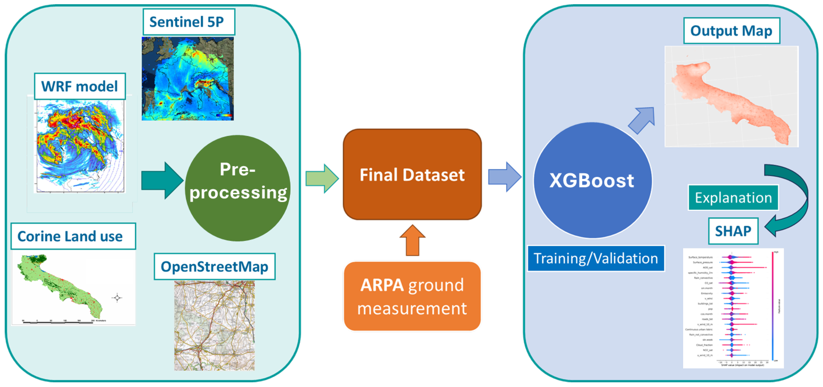
Figure 1 shows the flowchart of our analysis. We implemented a spatial preprocessing procedure to interpolate missing data, improve spatial resolution, perform spatial and temporal aggregation of input variables, and reproject the data to the chosen reference system. Subsequently, ground-based measurements from ARPA monitoring stations, which serve as ground truth, have been integrated. After creating the final dataset, we developed a machine learning analysis using the XGBoost model in a 5-fold cross validation framework to generate predictive maps for the entire area of interest. Finally, we interpreted the model’s decisions through an Explainable AI (XAI) analysis using the SHAP algorithm.

All the variables used to build the Machine Learning model with the spatio-temporal resolution and the source of the predictors are shown in

Table 1. List of all variables used to build the AI model. The Date and cell_id are used only to merge and aggregate data.

Name	Source/Product	Spatio–Temporal Resolution
U_wind_component	WRF	$4\mathrm{k}\mathrm{m}$, hourly
V_wind_component	WRF	$4\mathrm{k}\mathrm{m}$, hourly
Wind_speed	Computed (from WRF)	$4\mathrm{k}\mathrm{m}$, hourly
Emissivity	WRF	$4\mathrm{k}\mathrm{m}$, hourly
Rain_convective	WRF	$4\mathrm{k}\mathrm{m}$, hourly
Rain_non_convective	WRF	$4\mathrm{k}\mathrm{m}$, hourly
Vertical_wind	WRF	$4\mathrm{k}\mathrm{m}$, hourly
Specific_humidity_2m	WRF	$4\mathrm{k}\mathrm{m}$, hourly
Surface_temperature	WRF	$4\mathrm{k}\mathrm{m}$, hourly
Cloud_fraction	WRF	$4\mathrm{k}\mathrm{m}$, hourly
Surface_pressure	WRF	$4\mathrm{k}\mathrm{m}$, hourly
AOD	Computed 1	$300\mathrm{m}$, daily
NO2_sat	S5P (TROPOMI)	$5.5\times 3.5{\mathrm{k}\mathrm{m}}^2$, daily
O3_sat	S5P (TROPOMI)	$5.5\times 3.5{\mathrm{k}\mathrm{m}}^2$, daily
Sin_month, Cos_month	Computed	daily
Sin_week, Cos_week	Computed	daily
Population	WorldPop	$100\mathrm{m}$ (static)
Roads_tot	OSM	$100\mathrm{m}$ (static)
Buildings_tot	OSM	$100\mathrm{m}$ (static)
CORINE classes	CORINE	$100\mathrm{m}$ (static)
Continuous urban fabric	CORINE	$100\mathrm{m}$ (static)
Discontinuous urban fabric	CORINE	$100\mathrm{m}$ (static)
Cell_id	Computed	$300\mathrm{m}$ (grid)
Date acquired	Metadata	daily

¹ Computed as described in Section 4 (preprocessing and 300 m downscaling).

. These predictors were selected to jointly capture the main physical and socio-environmental drivers of surface pollution: emission intensity and urban form (population, roads, buildings, land cover), atmospheric transport and mixing/oxidation conditions (wind, stability proxies, humidity, clouds, precipitation, temperature, and pressure), regional background loadings from column satellite products (NO₂, O₃, and AOD), and recurrent temporal cycles (weekly/seasonal). Selection also prioritized variables with consistent regional coverage, minimal missingness, and the finest available resolution, while avoiding perfectly collinear duplicates. Additional details on dataset cardinality (number of rows/columns and file size) and feature-level missing-value percentages are provided in the Supplementary Materials.

2.1. Overall Workflow and Learning Dataset Construction

The supervised learning dataset is constructed as a station-day table: each row corresponds to one monitoring station and one day, the target is the daily pollutant concentration measured by ARPA stations ($\mathsf{\mu }$g/${\mathrm{m}}^3$), and predictors are extracted on the same day at the station location from gridded covariates. All predictors are harmonized to a common 300 m grid in the study CRS. Static layers (WorldPop, OSM, and CORINE) are aggregated to 300 m, WRF fields are aggregated from hourly to daily before spatial resampling, and Sentinel-5P and AOD daily rasters are reprojected to the grid. We adopt a 300 m grid as a compromise between resolving intra-urban gradients relevant for exposure assessment (e.g., traffic corridors and coastal industrial belts) and maintaining model stability given predictor availability and monitoring density. Missing values in satellite-derived predictors are gap-filled through a spatial interpolation ensemble. Model training and evaluation follow two strategies: repeated random cross-validation to estimate average predictive skill and a Leave-One-Year-Out protocol to assess temporal transferability.

2.2. Area of Interest

The area of interest is the Apulian region. This region is situated in the southern part of Italy, between approximately 41°${53}^{\prime }$ N and 39°${29}^{\prime }$ N latitude, and between 15°${33}^{\prime }$ E and 18°${31}^{\prime }$ E longitude. The region covers an area of about 19,541 square kilometers, making it one of Italy’s larger regions. It is divided into six provinces: Bari, Barletta-Andria-Trani, Brindisi, Foggia, Lecce, and Taranto. From an environmental perspective, Puglia is rich in biodiversity but also faces significant challenges.

Apulia has a Mediterranean climate, with hot and dry summers and milder, wetter winters. The coastal setting favors frequent sea and land breeze circulations and recirculation patterns that modulate dilution and transport. These mechanisms influence primary pollutants through ventilation and stagnation regimes, and they are also relevant for ozone because photochemistry is enhanced in warm and sunny conditions while coastal recirculation can sustain aged air masses.

One of the most critical environmental concerns centers around Taranto, an industrialized city that is home to one of Europe’s largest steel plants, ILVA.

Beyond the Taranto industrial area, Apulia includes additional relevant emission contexts. Traffic-related emissions dominate the main urban corridors and ring roads of coastal cities, while ports and shipping, together with logistics activities, contribute along the coastline. During winter, domestic heating can increase primary pollutants, and for particulate matter, the regional burden can also be affected by resuspension and episodic natural contributions (e.g., dust outbreaks), which increase day-to-day variability.

We focus on Apulia not only as a challenging coastal-industrial case study, but also because ongoing regional projects motivate One Health analyses that link high-resolution exposure fields with complex health outcomes at a local scale.

2.3. Data

2.3.1. ARPA’s Ground Control Units

The ARPA (Regional Environmental Protection Agency) is a public Italian organization dedicated to environmental monitoring [26]. Each Italian region operates its own regional agency, totaling 20 agencies. ARPA is also involved in air quality monitoring, deploying various types of sensors across Italy. These sensors can be fixed or mobile and are situated in specific areas: urban, suburban, rural, industrial, and traffic zones. Utilizing different detection systems (electrochemical sensors, optical particle counters, and ultraviolet photometric analyzers), ARPA provides hourly measurements of major atmospheric pollutants. These measurements, reported in micrograms per cubic meter ($\mathsf{\mu }$g/${\mathrm{m}}^3$), offer reliable estimates of human exposure to pollutants. The ARPA network in Puglia is fully compliant with national and European regulations, ensuring the necessary coverage and providing high-quality data for air quality assessment. 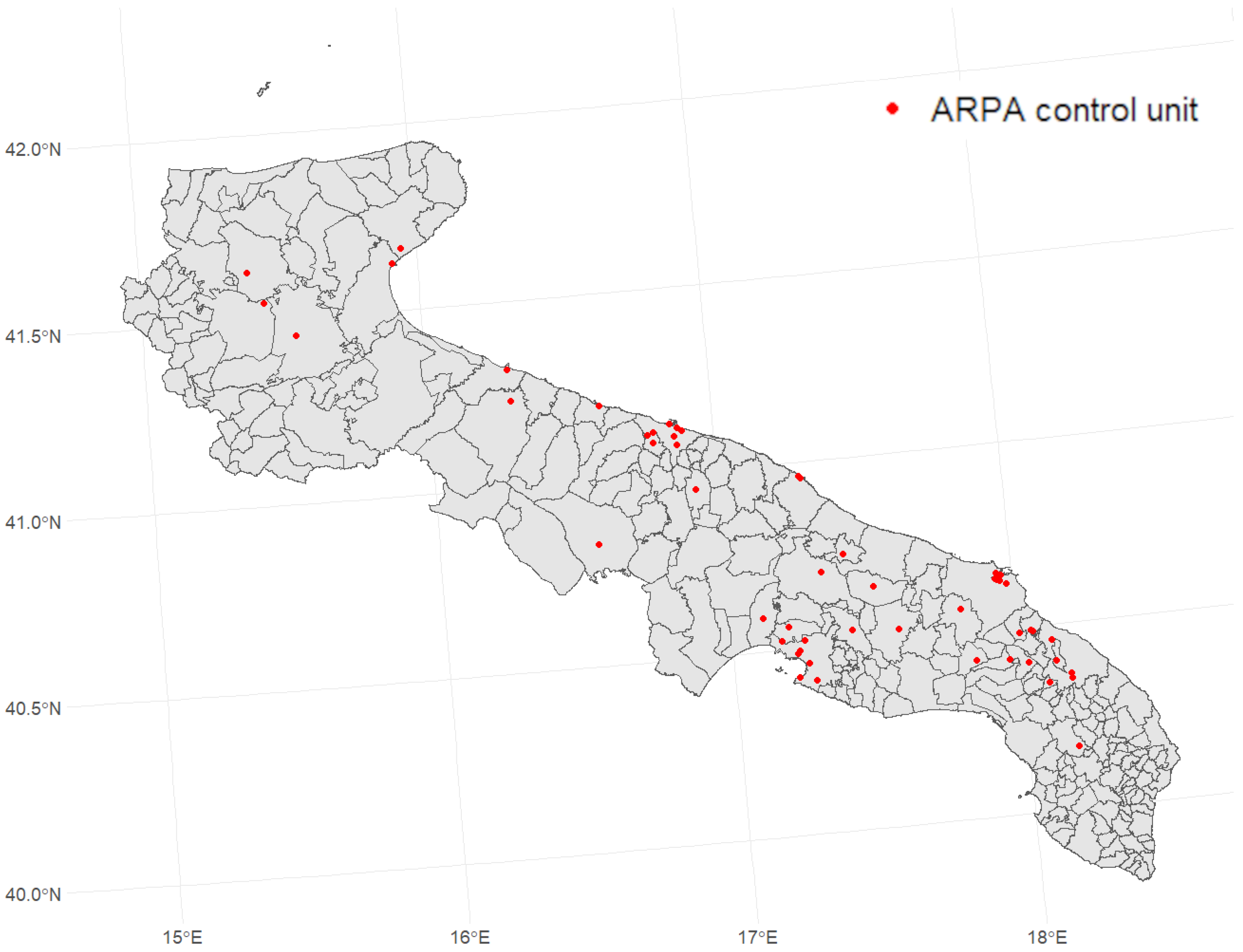The new European Air Quality Directive, adopted on 23 October 2024 and published in the Official Journal of the European Union on 20 November 2024, does not promote an increase in the number of stations but rather aims to optimize the existing network and strengthen the role of assessment modeling to achieve a more efficient analysis of air pollution [27]. For this purpose, starting from the ARPA stations in Puglia (52 for NO₂, 17 for O₃, 53 for PM₁₀, and 27 for PM_2.5), we developed a pipeline, based on machine learning applications, for comprehensive air quality assessment and modeling. In Figure 2 are shown the locations of all control units in Puglia.

2.3.2. Sentinel-5P

Sentinel-5P (Sentinel-5 Precursor) is a satellite mission launched by the European Space Agency (ESA) in October 2017 as part of the Copernicus Earth observation program [28]. Its primary mission is to monitor atmospheric composition and provide critical data on air quality, climate, and the ozone layer. Sentinel-5P is equipped with the TROPOspheric Monitoring Instrument (TROPOMI), an advanced spectrometer that measures a wide range of atmospheric gases, including nitrogen dioxide (NO₂), ozone (O₃), sulfur dioxide (${\mathrm{S}\mathrm{O}}_2$), carbon monoxide (CO), methane (CH₄), formaldehyde (HCHO), and aerosols, with a spatial resolution of up to 3.5 × 7 ${\mathrm{k}\mathrm{m}}^2$ at nadir. The satellite provides near-daily global coverage, with its orbit ensuring that nearly every location on Earth is observed at least once per day.

In our work, we used the tropospheric NO₂ and O₃ variables provided by the Sentinel-5P dataset. The images were downloaded from the Google Earth Engine platform, with a daily temporal resolution. These variables represent the surface density of these pollutants (expressed in mol/${\mathrm{m}}^2$), from ground level up to the troposphere. Therefore, these measurements do not account for the effects of urban microclimates and are consequently different from ground-based measurements. They are a good indicator of the presence of atmospheric pollutants, but do not provide data as accurate as the measurements from control units.

Specifically, for O₃ and NO₂ we used the Sentinel-5P Level-3 tropospheric_o3 and tropospheric_no2 bands accessed via Google Earth Engine; given our data-driven approach, no additional vertical correction or profile adjustment was applied beyond projection to the study reference system. Specifically, we found a Pearson correlation coefficient of 0.28 between surface NO₂ and the tropospheric NO₂ column, and 0.10 between surface and tropospheric O₃.

The relatively low ground-to-column correlations are physically expected because tropospheric columns are vertically integrated quantities and only indirectly reflect near-surface exposure, especially for O₃. In practice, this mismatch motivates the present data-fusion approach: if tropospheric columns were strongly and consistently correlated with surface concentrations, using the satellite products alone would already provide an adequate surface proxy.

Both dataset can be found at https://developers.google.com/earth-engine/datasets/catalog/COPERNICUS_S5P_OFFL_L3_NO2 (accessed on 10 February 2026) and https://developers.google.com/earth-engine/datasets/catalog/COPERNICUS_S5P_OFFL_L3_O3 (accessed on 10 February 2026).

2.3.3. Aerosol Optical Depth

Aerosol Optical Depth (AOD) is a satellite-derived parameter that quantifies the degree to which suspended particles in the atmosphere affect light transmission through absorption or scattering [29]. It serves as an indirect measure of aerosol concentration in the atmospheric column at a given time and location and is commonly used to estimate particulate matter concentrations ($P{M}_s$) [30].

Numerous satellite products provide AOD measurements at varying spatial and temporal resolutions. However, high-resolution AOD retrievals are often subject to artifacts, cloud contamination, and regional biases [31]. To address these limitations and improve the accuracy of daily AOD predictions over Italy, we developed a calibrated model that integrates multiple satellite and reanalysis products as predictors. These include 300 m Sentinel-3 SYN Aerosol Optical Depth at 550 nm [32], 1 km MODIS MAIAC AOD at 440 nm [33,34], 0.5° × 0.625° MERRA2 AOD reanalysis at 440 nm [35], and 0.75° × 0.75° CAMS AOD reanalysis at 440 nm [36].

We decided to use the AOD measurement at different wavelengths to add variability to the model and avoid highly correlated variables. In fact, these features could cause overfitting and strong fluctuations in model output and interpretability problems [37]. Auxiliary predictors, such as the 1 km MODIS Land Surface Temperature (LST) product, the Shuttle Radar Topography Mission (SRTM) Digital Elevation Model [38], ERA5 weather reanalysis variables (e.g., T2m, wind10m, etc.) [39], and geographical coordinates (latitude and longitude) were also included in the analysis.

For calibration, we relied on an extensive dataset of ground-based AOD measurements collected from 27 AERONET stations distributed across the Italian peninsula [40]. These measurements, spanning from January 2019 to December 2022, provided approximately 4300 data points, which served as true labels for calibrating and evaluating satellite-derived AOD products. Our methodology was inspired by Aldabash et al. [41], allowing us to quantitatively assess and refine model performance using this robust observational dataset.

The AOD calibration intentionally combines products with different native spatial resolutions. Higher-resolution satellite retrievals contribute spatial detail, while coarser reanalysis products provide temporally stable background information and help reduce gaps. All AOD predictors are harmonized to the common 300 m grid before calibration and use in the pollutant models, and calibration against AERONET helps mitigate resolution-driven artifacts and smoothing effects.

To integrate these observations with satellite and reanalysis data, we applied a stepwise calibration process based on an Ordinary Least Squares (OLS) linear regression model.

In the stepwise OLS calibration, candidate predictors were retained only if they improved generalization under a leave-one-station-out evaluation (to reduce spatial overfitting across sites). The final model retained the AOD products that provided the most stable cross-validated agreement with AERONET, while other candidates showed limited incremental contribution.

After extensive testing, the best-fitting solution incorporated MODIS MAIAC, CAMS, and MERRA2 AOD products as predictors, achieving a high level of agreement with AERONET observations ($R^2$ = 0.87) under a leave-one-station-out validation framework.

Further details regarding the analysis are provided in the Supplementary Materials. To ensure spatial consistency and comparability, all variables were resampled and projected onto a common 300-m grid. AOD processed data used in this study are available upon request.

2.3.4. Corine Data

The Corine Land Cover (CLC) dataset, developed by the European Environment Agency (EEA), provides comprehensive land use and land cover for all European countries. Based on satellite imagery, it classifies the landscape into over 40 categories, including urban areas, forests, and water bodies. The dataset has a spatial resolution of 100 m, which is comparable with the spatial resolution of our model [42].

In our analysis, we used the 5 macro-categories of Corine (1-Artificial surfaces, 2-Agricultural areas, 3-Forest, 4-Wetlands, and 5-Water bodies) to assign land cover classes to our area of interest. Additionally, we calculated the percentage of industrial area occupancy per pixel to identify patterns related to pollutant emissions, particularly NO₂. Oiamo et al. showed the influence of industrial areas in the prediction of different pollutants, including NO₂ [43].

We adopted five macro-categories because several fine CORINE sub-classes are absent or too sparse in the study area at the working resolution, which would increase sparsity and collinearity and reduce model stability. To retain source-relevant urban information, we also include targeted descriptors such as continuous and discontinuous urban fabric and an industrial occupancy indicator.

Data can be downloaded from https://developers.google.com/earth-engine/datasets/catalog/COPERNICUS_CORINE_V20_100m (accessed on 10 February 2026).

2.3.5. Weather Research and Forecasting Model

Meteorological inputs were produced using the Weather Research and Forecasting (WRF) model, configured over a single domain covering the Apulia region (latitude range 39.61°–42.41° N; longitude range 14.38°–18.97° E). The horizontal resolution was 4 km, with outputs stored at an hourly temporal resolution. The dataset spans the period from 31 December 2018, 12:00 UTC, to 3 January 2023, 00:00 UTC. Each simulation run covered 181 h; however, the first 12 h of each run were discarded to allow for model spin-up and stabilization. Boundary and initial conditions were taken from the ECMWF analysis dataset (0.16° horizontal resolution, 6-h temporal resolution). Land cover information was provided by the CORINE Land Cover database.

Table 2. WRF model domain and run configuration used in this study.

Item	Description
Model version	WRF (operational setup used by ARPA Puglia)
Domain extent	Apulia region (39.61°–42.41° N; 14.38°–18.97° E)
Horizontal resolution	4 km
Temporal resolution	Hourly output
Simulation period	31 December 2018, 12:00 UTC–3 January 2023, 00:00 UTC
Run length	181 h per forecast cycle
Spin-up removal	First 12 h of each cycle discarded
Lateral/initial forcing	ECMWF analysis (0.16°; 6-hourly)
Land cover dataset	CORINE Land Cover
Output variables	3D atmospheric state (U, V, W, T, water species);
	surface fields (PSFC, T2, U10, V10, PBLH, radiation fluxes, precipitation);
	soil variables (soil temperature, soil moisture, runoff)
Post-processing for this work	Hourly → daily aggregation; vertical averaging of selected variables (e.g., vertical wind) to reduce redundancy; resampling to 300 m grid via cubic interpolation (Section 2.4.1); projection to the study CRS

summarizes the WRF domain configuration and runtime settings adopted in this study.

The physical parameterization schemes used in the WRF simulations are reported in

Table 3. WRF physical parameterizations adopted in this work. The right column reports the corresponding namelist.input options.

Process	Scheme	WRF Option
Microphysics	Thompson	mp_physics = 8
Longwave radiation	RRTM	ra_lw_physics = 1
Shortwave radiation	Dudhia	ra_sw_physics = 1
Planetary Boundary Layer (PBL)	YSU	bl_pbl_physics = 1
Surface layer	Monin–Obukhov	sf_sfclay_physics = 1
Land surface model	Noah LSM	sf_surface_physics = 2
Cumulus parameterization	Kain–Fritsch	cu_physics = 1

. These choices follow the operational configuration validated for the Apulia region.

Validation. The adopted WRF configuration (including CORINE land cover and the physics schemes in Table 3) has been previously tested and validated over the Apulia region. In particular, Fedele et al. (2015) analyzed spatial biases in WRF simulations with focus on Apulia [44]; Fedele et al. (2015, EMS/ECAM) investigated how different PBL schemes and land cover classifications affect wind speed and temperature biases [45]; Tateo et al. (2017) evaluated ensemble simulations with alternative PBL schemes for wind speed and direction prediction [46]; and Tateo et al. (2018) assessed PBL height prediction using multi-physics ensembles [47]. These studies support the robustness of this setup, which is also used operationally by ARPA Puglia for forecasting and Wind Day alerts.

Finally, all WRF raster outputs were projected to the study reference CRS. The resampled daily fields were then integrated with Sentinel-5P, AOD, land-use (CORINE, OSM), WorldPop population density, and temporal harmonics to build the final machine learning dataset.

To contextualize the meteorological drivers used in the model, we report in the Materials section summary statistics (mean and min–max) of the main WRF-derived predictors over the study period, which describe the seasonal variability relevant for dispersion and photochemistry.

Table 4. Summary statistics of main WRF predictors over Apulia (2019–2022) after daily aggregation.

Variable	Mean	Min	Max
Wind speed (m ${\mathrm{s}}^{-1}$)	2.73	0.01	15.76
Surface temperature (K)	292	269	312
Surface pressure (hPa)	1007.5	944.5	1039.3
Specific humidity 2 m (kg ${\mathrm{k}\mathrm{g}}^{-1}$)	0.009	0.002	0.020
Precipitation (convective + not convective) (mm ${\mathrm{d}\mathrm{a}\mathrm{y}}^{-1}$)	5.70	0	283.48

shows the main WRF predictors stats over Apulia.

2.3.6. OpenStreetMap Data

OpenStreetMap (OSM) is a collaborative, open-source project that provides free and editable geographic data, created and maintained by a global community [48]. It offers detailed mapping information, including roads, buildings, land use, and natural features, making it a valuable resource for applications in geographic information systems (GIS), navigation, urban planning, and environmental monitoring [49].

Specifically, from the OSM website, we downloaded two shapefiles containing both the locations of all buildings and all roads for the whole Apulia territory. From the first file, we calculated the total number of buildings within each considered grid cell, while from the second file, we computed the total length of roads intersecting each cell. Data can be found here: https://download.geofabrik.de/europe/italy.html (accessed on 10 February 2026).

OSM-derived indicators and CORINE land cover can partially overlap in the urbanization signal, but they capture complementary aspects: roads and buildings from OSM versus categorical land cover from CORINE. We therefore retain both while keeping land-cover encoding parsimonious to limit redundancy.

2.3.7. Population Data

To make a model as general as possible, we added information regarding the urban effect. Specifically, we used the dataset provided by WorldPop [50]. This dataset, in GeoTIFF format, contains an estimate of the population in the Italian territory, with a grid resolution of 100 m. The mapping method employed to build the dataset is the Random Forests-based dasymetric redistribution technique developed by Stevens et al. [51]. We extracted values using our reference grid, applying the sum function as the aggregation method at 300 m. Data are available at https://developers.google.com/earth-engine/datasets/catalog/WorldPop_GP_100m_pop (accessed on 10 February 2026).

2.4. Preprocessing

2.4.1. Spatial Resample of WRF Data

The procedure of converting a sampled image from any coordinate structure to another structure is called image resampling. This is a complicated process that involves several geometric transformations of an image and can be summarized in three main steps:

• reconstruction of a continuous intensity surface from a discrete image;
• transformation of the continuous surface into the new coordinate system;
• sampling of the transformed surface to create a new discrete image.

In our analysis, we had to transform the WRF data structure into our prediction grid and increase the resolution of the model to 300 m. The first step consisted of a spatial interpolation of the original raster image.

Among the three methods described in [52], we chose the Bi-Cubic Interpolation method, which provides smoother results, especially compared to the Bi-Linear Interpolation. This method considers a 4 × 4 grid of surrounding pixels and performs a convolution with the kernel function given in the Equation (1) [53]. This allows for more accurate and natural-looking transitions between pixel values, reducing artifacts like blurring or jagged edges.

$$u\left(x\right)=\left\{\begin{array}{cc}{\displaystyle \frac{3}{2}}{\left|x\right|}^3-{\displaystyle \frac{5}{2}}{\left|x\right|}^2+1\hfill & \hfill 0<\left|x\right|<1\\ -{\displaystyle \frac{1}{2}}{\left|x\right|}^3+{\displaystyle \frac{5}{2}}{\left|x\right|}^2-4\left|x\right|+2\hfill & \hfill 1<\left|x\right|<2\\ 0\hfill & \hfill \left|x\right|>2\end{array}\right.$$

(1)

The method is particularly used for continuous data, such as satellite imagery or elevation models [54], where maintaining smooth transitions is important, even if it can sometimes introduce slight overshooting where there are sharp changes in the data. The Supplementary Materials include example figures showing surface emissivity, as predicted by the WRF model, before and after applying the resampling method. 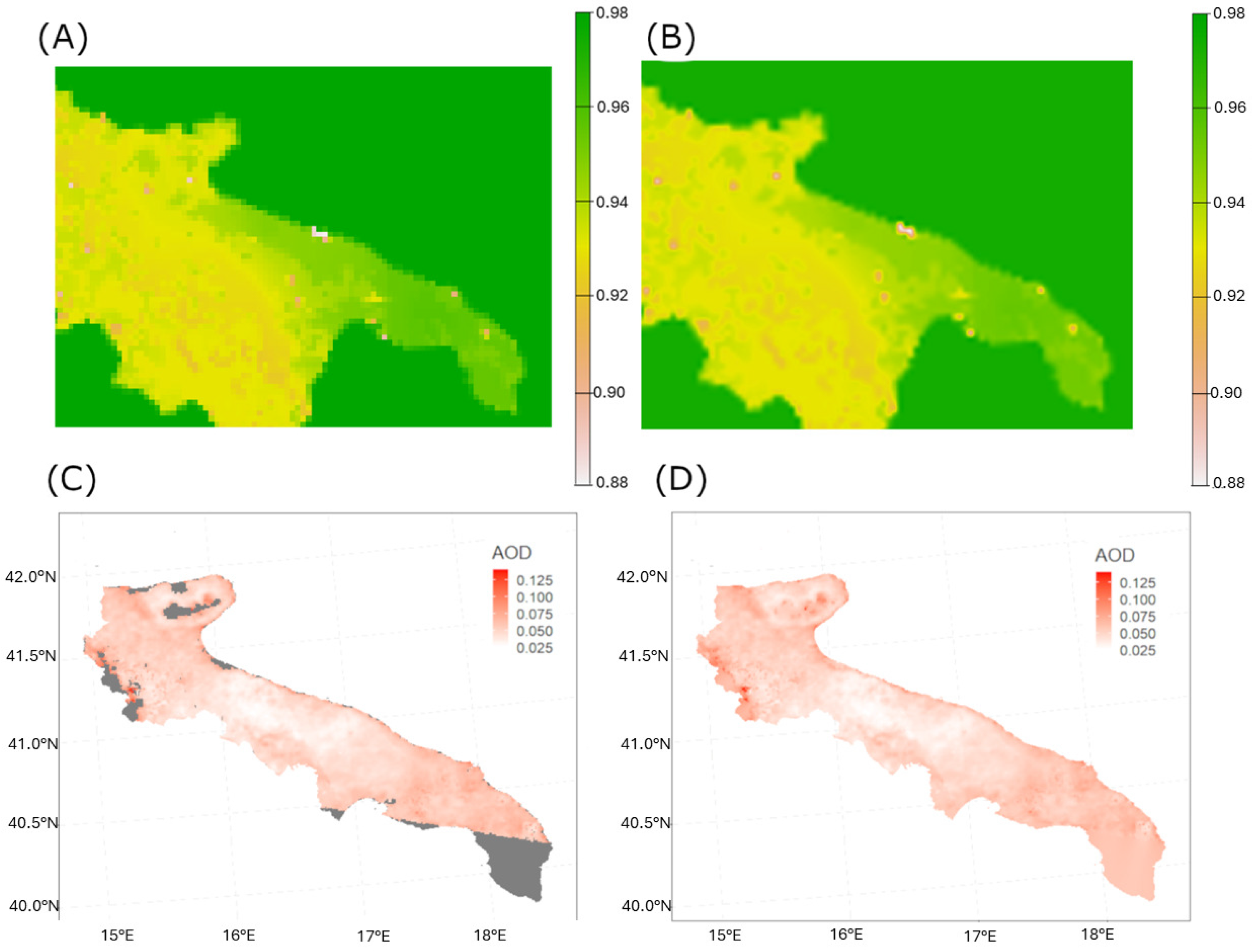Figure 3 shows the Surface Emissivity (WRF) before (panel (A)) and after (panel (B)) the resampling.

2.4.2. Spatial Interpolation for Missing Data

As we have described in the previous section, spatial interpolation is a statistical method used to estimate the values of a variable at unsampled locations based on the values observed at known points [55].

In this analysis, we filled the missing values of the input data by using an ensemble approach that combines the predictions obtained with several spatial interpolation methods [56]. This is essential for the Sentinel-5P and AOD data, which contain large gaps due to orbital constraints or cloud cover. The missing values are estimated by averaging the Inverse Distance Weighting (IDW) and the Nearest Neighbors (NN) interpolation methods. An example of this procedure’s results is shown in the Supplementary Materials. Figure 3 shows the AOD values before (panel (C)) and after (panel (D)) the spatial interpolation.

2.4.3. Inverse Distance Weighting

Inverse Distance Weighting (IDW) is a widely used spatial interpolation technique that estimates the value of a variable z at an unsampled location $x_0$ through a weighted average of values at sampled points $x_i$ as shown in Equation (2) [56].

$$z\left(x_0\right)={\displaystyle \frac{{\sum }_{i=1}^n{w}_{i}z\left(x_i\right)}{{\sum }_{i=1}^n{w}_i}}$$

(2)

The underlying assumption of the IDW method is that points closer to the location of the prediction have a greater influence than points further away. Therefore, the weight assigned to each sample point is inversely proportional to its distance from the prediction location. Furthermore, these distances can be raised to a power parameter $\beta \ge 0$ that controls the rate of decline of influence with distance, as shown in Equation (3):

$$w_i=d_{Euclidean}^{-\beta }\left(x_0,x_i\right)$$

(3)

Typical values for $\beta$ are 1 or 2, corresponding to an inverse or quadratic relationship respectively, in our analysis we have assigned $\beta =1$.

2.4.4. Nearest Neighbors

The NN interpolation method is another technique in which the value of a variable z at an unsampled location $x_0$ is determined using the average of the k nearest points to that location, as shown in Equation (4).

$$z\left(x_0\right)={\displaystyle \frac{{\sum }_{i=1}^{k}z\left(x_i\right)}{k}}$$

(4)

This method is based on the assumption that only the points closest to the target location can be considered for the prediction of the variable value. In this case, we choose k to be equal to the rounded square root of the number of sampled cells.

2.5. ML Analysis

Nowadays, ML methods are growing in popularity and are used in many fields to capture the complex data dependencies. In our analysis, we compared the results obtained from two different ML algorithms: linear regression and eXtreme Gradient Boosting (XGBoost).

We selected linear regression as a transparent baseline model and XGBoost as a state-of-the-art tree-ensemble for heterogeneous tabular predictors. This choice is motivated by the expected non-linearities and interaction effects among satellite columns, meteorology, land-use proxies, and temporal harmonics in atmospheric processes, and by the need for post hoc interpretability through TreeSHAP.

The XGBoost model is an ensemble method consistently used to study several problems thanks to its scalability in all scenarios [57]. The algorithm is faster than other machine learning techniques and and scales to billions of examples in distributed or memory-limited settings [58].

XGBoost is composed of tree models that use a series of cumulative functions to predict the output of a certain task as shown in Equation (5):

$$\widehat{y_i}=\Phi \left({\mathbf{x}}_i\right)=\sum _{k=1}^K{f}_k\left({\mathbf{x}}_i\right),f_k\in \mathcal{F}$$

(5)

where $\mathcal{F}$ is the space of the Classification and Regression Trees (CART). The parameters of the model are optimized in order to minimize a regularized object, which is a sum of the loss function l and a factor expressing the complexity of the model $\Omega$, as shown in Equation (6):

$$\mathcal{L}(\Phi )=\sum _{i=1}^{N}l\left(\widehat{y_i},y_i\right)+\sum _{k=1}^K\Omega \left(f_k\right)$$

(6)

Another important procedure that characterizes the XGBoost model is shrinkage. This procedure scales newly added weights by a factor $\eta$ after each step of tree boosting to reduce the influence of each individual tree and leaves space for future trees [59]. Furthermore, XGBoost implements feature sub-sampling during the training phase, which makes it robust to the over-fitting problem and speeds up the computations.

2.6. Performances Metrics

To assess the performances of our model we used three different metrics:

• the mean absolute error (MAE), defined as

  $$MAE={\displaystyle \frac{1}{n}}\sum _{i=1}^N\left|y_i-\widehat{y_i}\right|,$$

  (7)
• the root mean square error (RMSE), defined as

  $$RMSE=\sqrt{{\displaystyle \frac{1}{n}}\sum _{i=1}^n{\left(y_i-\widehat{y_i}\right)}^2}$$

  (8)
• the coefficient of determination between predicted and actual values

  $$R^2=1-{\displaystyle \frac{{\sum }_{i=1}^N{\left(y_i-\widehat{y_i}\right)}^2}{{\sum }_{i=1}^N{\left(y_i-\overline{y}\right)}^2}},$$

  (9)

  with $y_i$ that represents the actual value, $\widehat{y_i}$ the predicted value and $\overline{y}$ la media dei valori reali.

2.6.1. Validation Strategy and Leakage Prevention

We adopted two complementary validation strategies. First, we used repeated random 5-fold cross-validation to estimate average predictive skill and reduce variance in performance estimates; reported metrics are computed from out-of-fold predictions only. Second, to assess temporal transferability, we used a Leave-One-Year-Out protocol: the model is trained on three years and tested on the held-out year, repeating the procedure so that each year is used once as a test set. For the linear regression baseline, any feature standardization is fitted on the training portion of each split only and then applied to the corresponding validation fold to prevent information leakage.

2.6.2. Hyperparameter Settings

XGBoost was trained using the standard regression objective. We retained default hyperparameter settings to enhance reproducibility, and we verified through a dedicated grid-search sensitivity analysis that the best-performing configurations were consistently close to the default setup under our validation scheme [60]. Additional details and full pollutant-specific grid-search results are provided in the Supplementary Materials.

2.7. Explainable Artificial Intelligence: SHAP

Explainable Artificial Intelligence (XAI) refers to a variety of techniques that try to improve transparency and generalization to several AI models [61,62].

In particular, in our study we used the SHAP (SHapley Additive exPlanations) local explanation method to assess the contribution of each feature within the XGBoost model. Using a game theory approach [63,64], SHAP estimates the contribution to the prediction of each predictor without knowing how the ML model works. An important characteristic of this technique is the ability to provide local explanation instead of the average explanations given by the XGBoost model. Finally, SHAP provides a link between the values of the predictors at the specific prediction and their contribution to the final output. Those correlations are shown in the SHAP importance plot.

Mathematically, given all possible feature subsets F of the total feature set S ($F\subseteq S$), for a feature j, the SHAP value is evaluated as the difference between two model outputs, the first obtained including that specific feature, the second without. The SHAP value of the j-th feature for the observation x is measured through the addition of the j-th feature to all possible subsets,

$$SHA{P}_j\left(x\right)=\sum _{F\subseteq S-\left\{j\right\}}{\displaystyle \frac{\left|F\right|!\left(\right|S|-|F|-1)!}{\left|S\right|!}}[f_x(F\cup j)-f_x\left(F\right)],$$

(10)

where $\left|F\right|!$ is the number of feature permutations that precede the j-th feature; $\left(\right|S|-|F|-1)!$ is the number of feature permutations that follow the j-th feature value; $\left|S\right|!$ represents the total number of permutations of features; $f_x\left(F\right)$ indicates the model prediction f for the sample x, considered a subset F without the j-th feature; $f_x(F\cup j)$ is the output of the same model including the j-th feature [63]. In our analysis we computed the mean SHAP values after a 5-fold CV, repeated 100 times for each considered year.

2.8. Software and Packages

The analyses were conducted using R version 4.4.1 (14 June 2024). The spatial analysis was carried out with the following packages: raster, terra, exactextractr, sf, stars, and gstat. Additionally, the analysis was parallelized using the doPar and foreach packages to accelerate data preprocessing. For the Machine Learning models, the packages XGBoost, Ranger, and caret were employed. The XAI analysis, on the other hand, was performed using Python 3.9.13 with the Spyder version 5 interface and the shap package.

3. Results

After the preprocessing phase, we developed two models for pollutant prediction. Specifically, we used linear regression as a benchmark model and an ensemble learning algorithm, XGBoost. As in our previous work, we found that the Random Forest model achieves similar performance to the XGBoost model but requires more computational time; therefore, we did not include it in the analysis [22].

Table 5. Random cross-validation (5-fold, repeated 10 times). Metrics are mean ± SD across repeats. MAE and RMSE in $\mathsf{\mu }\mathrm{g}{\mathrm{m}}^{-3}$. All p-values are significant at the 1% level.

	MAE	RMSE	R2
	($\mathsf{\mu }$g m−3)	($\mathsf{\mu }$g m−3)
Linear model
NO2	$5.60\pm 0.01$	$7.42\pm 0.01$	$0.39\pm 0.01$
O3	$11.17\pm 0.01$	$14.4\pm 0.01$	$0.50\pm 0.01$
PM2.5	$4.36\pm 0.01$	$5.94\pm 0.01$	$0.18\pm 0.01$
PM10	$6.91\pm 0.01$	$9.49\pm 0.01$	$0.18\pm 0.01$
XGBoost
NO2	$3.21\pm 0.01$	$4.52\pm 0.01$	$0.77\pm 0.01$
O3	$7.29\pm 0.01$	$9.48\pm 0.01$	$0.78\pm 0.01$
PM2.5	$2.66\pm 0.01$	$3.74\pm 0.01$	$0.67\pm 0.01$
PM10	$4.45\pm 0.01$	$6.26\pm 0.01$	$0.64\pm 0.01$

reports the performance metrics evaluated during the training phase.

Table 5 shows that XGBoost substantially outperforms the linear model for all pollutants in random 5-fold CV repeated 10 times. For NO₂, $R^2$ increases from $0.39$ (linear) to $0.77$ (XGBoost), with a mean absolute error (MAE) reduction of about 2.4 $\mathsf{\mu }$g/${\mathrm{m}}^3$. PM₁₀ and PM_2.5 also benefit from the non-linear model, with $R^2$ rising from 0.18 (linear) to 0.64 and 0.67, respectively. This indicates that particulate matter fields are strongly driven by non-linear interactions among satellite-based AOD, meteorology, and land-use variables, which are not captured by a purely linear formulation. For O₃, the $R^2$ reaches $0.78$, confirming that, despite the known weak linear relationship between tropospheric column O₃ and surface O₃, the model can still recover useful predictive structure once meteorology and temporal features are included. Overall, random CV demonstrates that tree-based fusion of satellite, meteorology, land-use and temporal harmonics provides accurate daily predictions at 300 m resolution.

Across pollutants, performance is differentiated. NO₂ and the particulate fractions (PM₁₀, PM_2.5) exhibit high accuracy and low RMSE, reflecting their strong link to localized emission patterns (traffic, industrial areas) and aerosol load, respectively. O₃ achieves similar apparent $R^2$ under random CV, but as we will discuss below, ozone behaves very differently under temporal generalization.

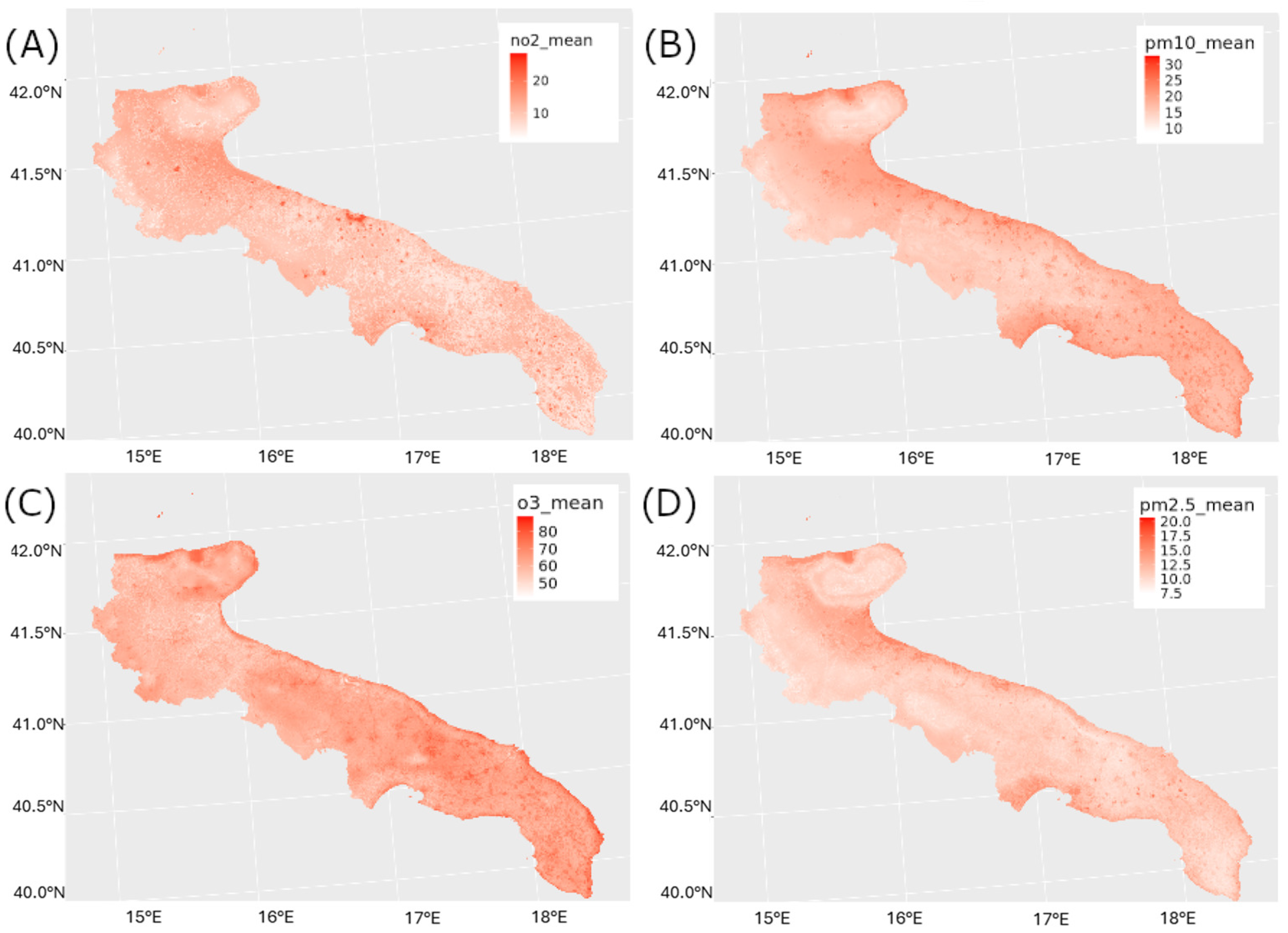
The results reported in Table 5 are obtained through a 5-fold cross-validation (CV) procedure repeated 10 times. After confirming that the XGBoost model performed better than the linear model, we predicted air quality (4 pollutants) for the entire territory of the Apulia region. Figure 4 shows the daily concentration of NO₂, O₃, PM₁₀, and PM_2.5 predicted by means of our framework and averaged over the considered time interval.

Spatially, the NO₂ map highlights dense urban/industrial corridors, especially around Bari and Taranto, with sharp intra-urban gradients at the 300 m scale. Particulate matter (PM₁₀, PM_2.5) shows broader plumes, including higher values in coastal and harbor/industrial areas, consistent with resuspension, port activity, and industrial processes. In contrast, O₃ appears more spatially homogeneous at a regional scale, with smoother inland gradients that reflect its secondary, photochemically formed nature and regional transport rather than purely local emissions. These spatial patterns are consistent with known atmospheric behavior of primary vs. secondary pollutants.

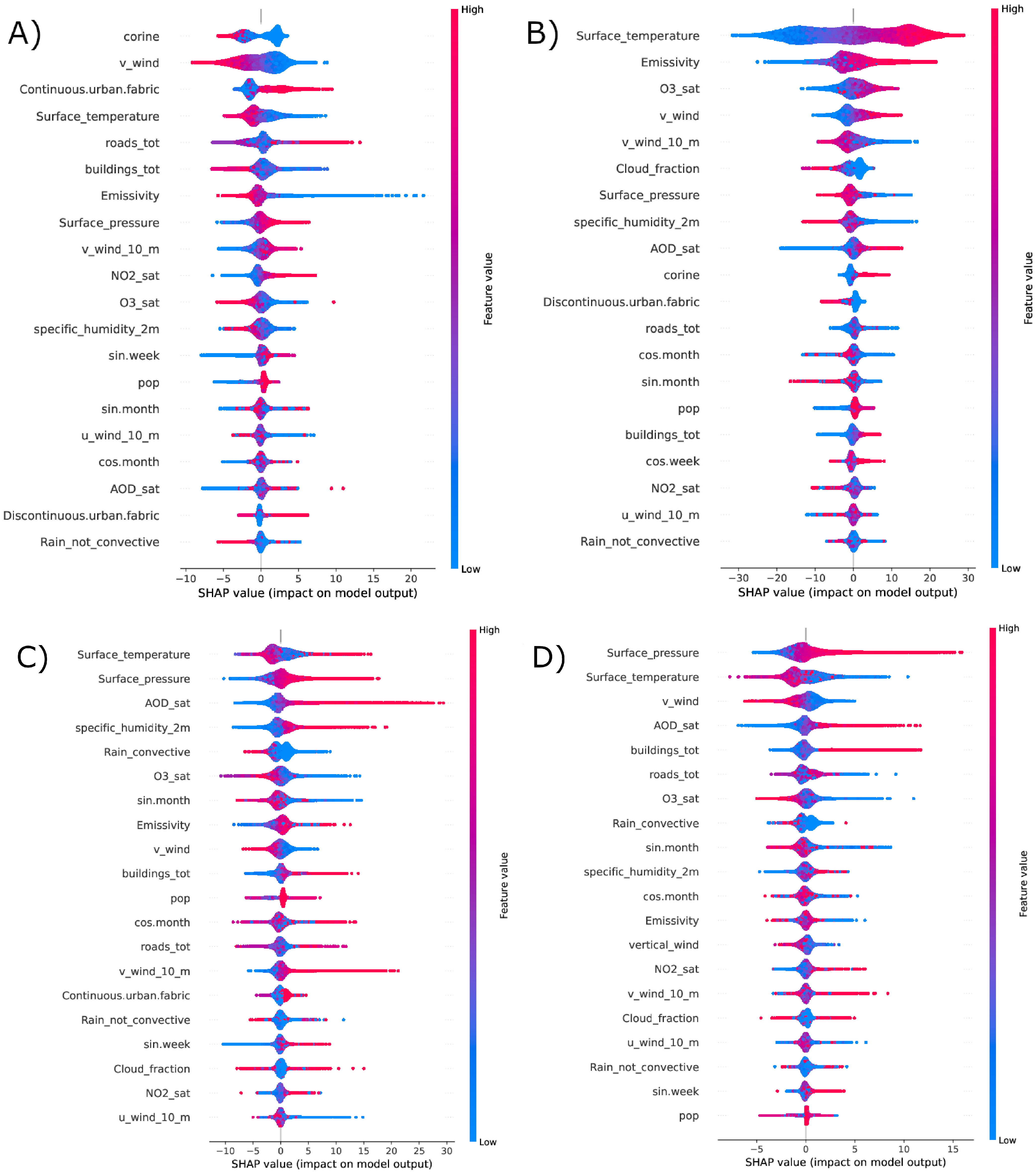
To better understand the reasoning behind the model’s predictions, we applied the SHAP algorithm, which highlighted the most influential variables and their relationship with the model’s output, as shown in Figure 5.

For NO₂, SHAP ranks land-use and anthropogenic predictors (road network density, built-up/industrial fabric from CORINE, population density) and meteorological dispersion variables (wind speed) among the top drivers. High road density and continuous urban fabric push predictions upward, pointing to traffic and industrial combustion as dominant local sources. Wind speed contributes with negative SHAP values at high intensity, consistent with dilution and advection away from sources. Temperature shows a generally negative contribution at higher values, in line with the known seasonal cycle of NO₂ (winter accumulation under stable conditions vs. enhanced mixing and photochemical removal in summer).

For PM₁₀ and PM_2.5, SHAP attributes a strong positive role to AOD, confirming that the calibrated multi-source AOD field encodes aerosol load relevant to surface PM. Meteorological variables such as wind and precipitation act in the expected direction: higher wind speed and rainfall tend to reduce predicted particulate levels through dispersion and wet scavenging. Land-use features (industrial/urban classes) also contribute positively, but their SHAP magnitude is generally lower than AOD and meteorology, reflecting the more regional nature of particulate burden.

For O₃, SHAP identifies temperature and emissivity (a proxy linked to surface energy balance and thus photochemical activity) as strong positive drivers, consistent with O₃ being formed photochemically under warm, sunny, stagnant conditions. Wind speed shows non-trivial effects, suggesting both transport and recirculation. Importantly, the Sentinel-5P tropospheric O₃ column appears as a meaningful predictor despite the low raw Pearson correlation (0.10) with ground-level O₃: SHAP indicates that the model leverages this satellite feature in interaction with meteorology and land cover, rather than as a simple linear proxy. This supports the view that non-linear ML is needed to extract surface-relevant information from column-integrated products.

We acknowledge that the raw Pearson correlation between the tropospheric O₃ column and surface O₃ is low (R ≈ 0.1), but low marginal linear correlation does not imply that a variable lacks predictive value in non-linear, interaction-based ensembles such as XGBoost. In gradient boosting, trees combine features hierarchically through splits and interactions, so a predictor can become informative conditionally, e.g., above specific temperature thresholds, under particular wind regimes or boundary-layer stability, or in locations with distinct land-use/${\mathrm{N}\mathrm{O}}_x$ availability, even if its global linear association with the target is weak. This is a well-established property of boosted trees and modern feature selection theory: univariate correlation is an unreliable proxy for utility in non-linear models, whereas embedded/wrapper approaches and post hoc attributions are preferred [57,58,65,66,67]. Consistently, TreeSHAP provides additive, locally accurate attributions for tree ensembles; in our O₃ model, SHAP assigns a non-negligible contribution to the Sentinel-5P column precisely when meteorology and land/emission proxies create favorable photochemical/background conditions, confirming interaction-driven use rather than any one-to-one mapping [63,64].

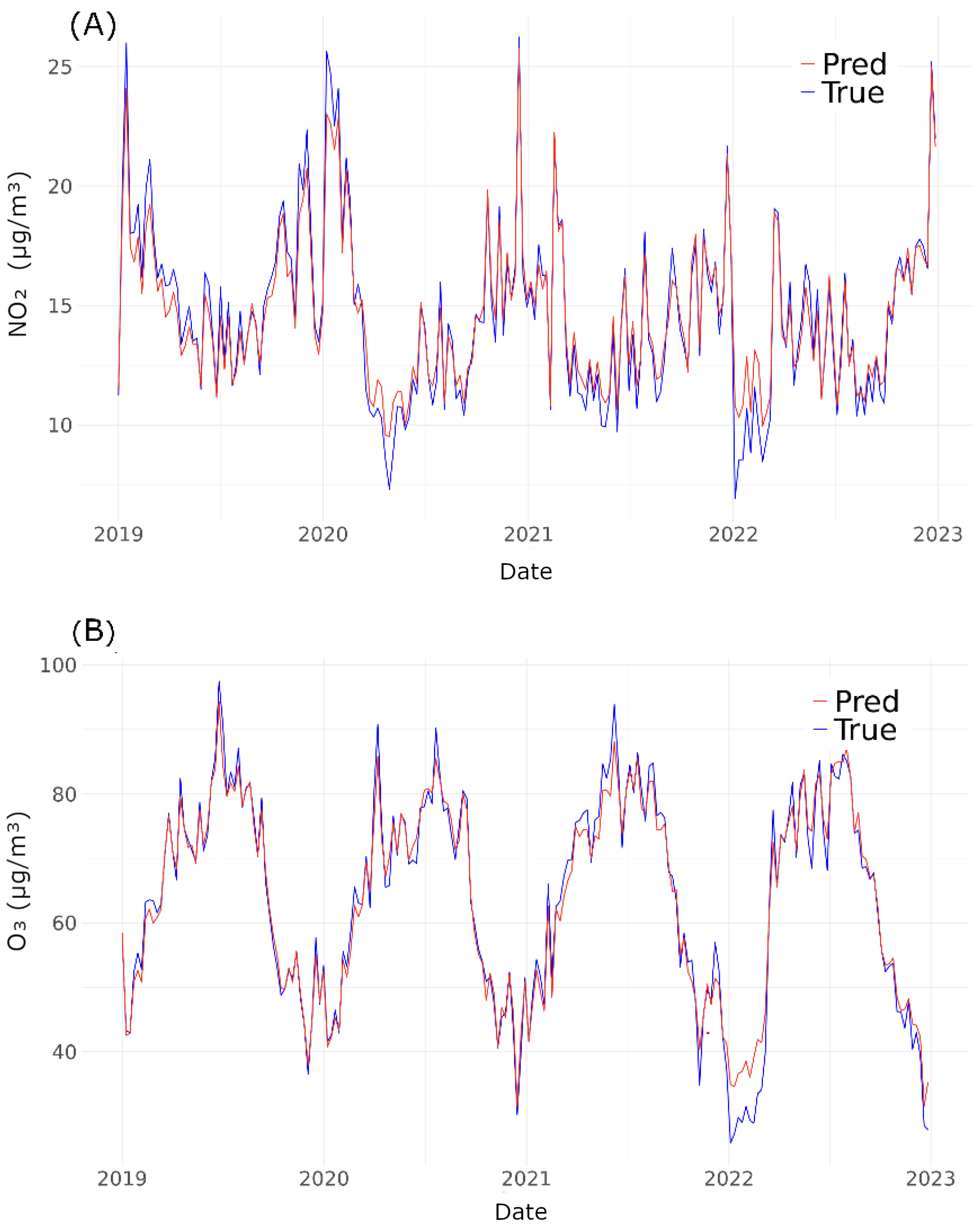
Figure 6 shows the trend of the predicted concentrations of NO₂ and O₃ compared to the ground values (our labels), averaged over all ground stations. To obtain this plot, we applied a Random CV procedure.

The temporal evolution in Figure 6 shows that the model reproduces the seasonal cycles of both pollutants. NO₂ peaks in winter and drops in summer, reflecting lower atmospheric mixing heights and more intense combustion/traffic demand in the cold season. O₃ instead peaks in the warm season, consistent with photochemical production under high temperature and radiation. The anti-correlation between the two is evident (high NO₂/low O₃ in winter and vice versa in summer) and is well captured by the model. The largest discrepancies between prediction and ground truth occur during extreme or transient episodes, which is expected given the limited number of ARPA monitoring stations and the fact that highly localized spikes (e.g., short-lived plumes and stagnation events) are harder to generalize regionally.

To assess the temporal generalization ability of the model, we adopted a different cross-validation approach. In particular, we applied a LOYO (Leave One Year Out) strategy, splitting the dataset by year.

In this procedure the model was trained for three years (we considered the time interval 2019–2022) and tested for the remaining year. This procedure was repeated to ensure that each year was used at least once for both testing and training.

Table 6. Leave-One-Year-Out (LOYO) cross-validation for the XGBoost model. Metrics are mean ± SD across LOYO folds. MAE and RMSE in $\mathsf{\mu }\mathrm{g}{\mathrm{m}}^{-3}$. Predictions are evaluated at a daily scale and after aggregation to monthly and annual means. All p-values are significant at the 1% level.

	MAE	RMSE	${\mathbf{R}}^2$
	($\mathsf{\mu }$g m−3)	($\mathsf{\mu }$g m−3)
Day prediction
NO2	$4.60\pm 0.40$	$7.05\pm 0.67$	$0.59\pm 0.05$
O3	$10.52\pm 1.77$	$13.51\pm 2.30$	$0.53\pm 0.03$
PM2.5	$3.92\pm 0.18$	$5.45\pm 0.26$	$0.30\pm 0.01$
PM10	$6.28\pm 0.36$	$8.70\pm 0.53$	$0.24\pm 0.06$
Month prediction
NO2	$3.28\pm 0.60$	$4.91\pm 0.99$	$0.76\pm 0.08$
O3	$6.36\pm 1.99$	$8.43\pm 2.92$	$0.72\pm 0.06$
PM2.5	$1.89\pm 0.14$	$2.39\pm 0.20$	$0.72\pm 0.05$
PM10	$3.06\pm 0.17$	$4.06\pm 0.24$	$0.51\pm 0.04$
Year prediction
NO2	$2.71\pm 0.78$	$3.88\pm 1.14$	$0.84\pm 0.05$
O3	$4.17\pm 1.66$	$4.99\pm 1.92$	$0.33\pm 0.15$
PM2.5	$1.42\pm 0.37$	$1.63\pm 0.41$	$0.79\pm 0.13$
PM10	$2.16\pm 0.49$	$3.35\pm 0.77$	$0.63\pm 0.03$

shows the performance metrics (MAE, RMSE, and $R^2$) obtained with this approach. Additionally, we summarized the predictions to monthly and yearly averages to observe possible seasonal trends. We decided not to perform spatial cross-validation (which is widely used in the literature), as the small number of measurement stations would lead to a bias in the model.

Table 6 evaluates a much harder task: predicting an unseen year (LOYO). As expected, daily-scale $R^2$ drops for all pollutants compared to random CV (Table 5), because LOYO tests temporal transferability under different meteorological regimes and emission patterns. NO₂ remains relatively robust ($R^2=0.59\pm 0.05$ daily), confirming that the model captures persistent spatial structure of primary emissions (traffic, industry). PM₁₀ and PM_2.5 show lower daily $R^2$ (0.24 and 0.30), which reflects their higher stochastic variability (episodic dust resuspension, Saharan intrusions, industrial events) and the limited number of monitors. Critically, O₃ exhibits $R^2=0.53\pm 0.03$ at a daily scale, lower than its random-CV $R^2=0.78$. This indicates that ozone is the least temporally transferable pollutant in our framework, consistent with the fact that O₃ depends on interannual meteorology and chemistry (photochemistry, $NO$ titration, boundary-layer recirculation), and that satellite O₃ columns capture large-scale background rather than purely local boundary-layer behavior.

However, when we aggregate predictions to monthly and yearly means, performance markedly improves for all pollutants. For example, NO₂ reaches $R^2=0.84\pm 0.05$ at the annual scale, and PM_2.5 reaches $R^2=0.79\pm 0.13$. Even O₃, while still more variable, reaches $R^2=0.72\pm 0.06$ at the monthly scale. This suggests that although day-to-day prediction of certain episodes is challenging across years, the model is robust for exposure assessment at epidemiologically relevant aggregation windows (monthly/annual), which are commonly used in long-term health and policy studies.

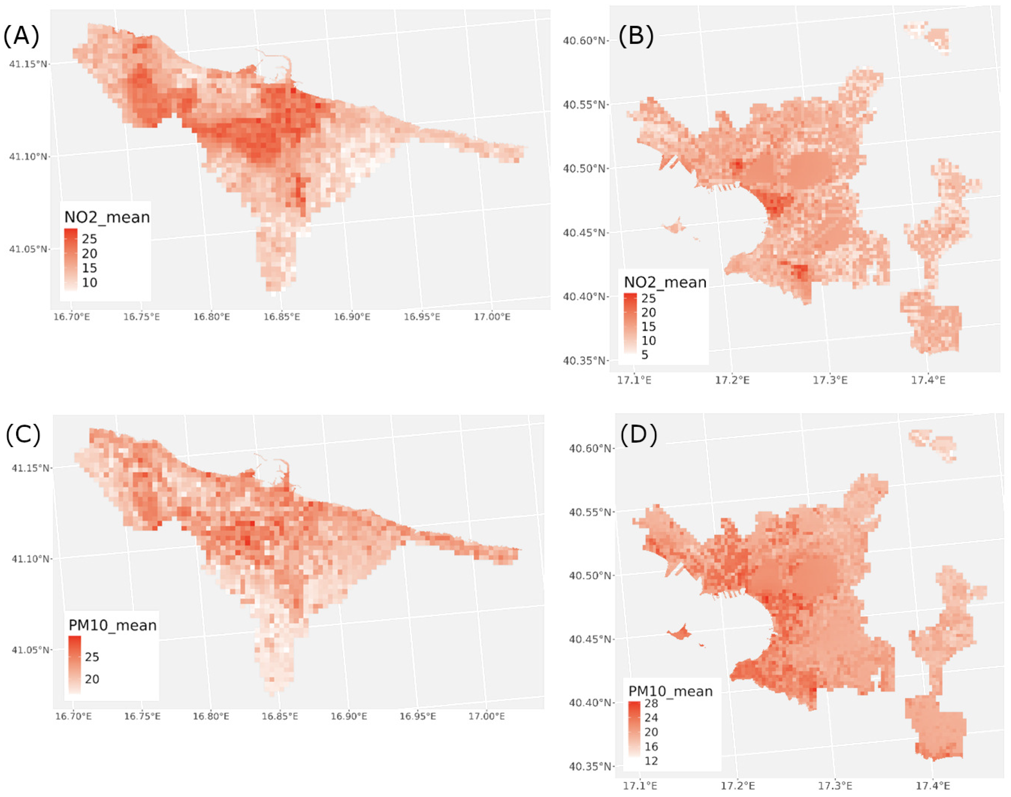
Through our model, we can produce maps at the municipality level to focus on more local realities. Figure 7 shows the average predicted values of NO₂ and PM₁₀ in the municipalities of Bari and Taranto, respectively.

In Bari, NO₂ hotspots align with dense road networks and industrial/port areas, consistent with traffic-related and combustion-related sources. PM₁₀ shows elevated levels both in industrial zones and along the coastline. This coastal enhancement is in line with AOD-informed particulate fields and may reflect port activity, industrial processes, and resuspension of marine/harbor aerosols. A similar pattern is observed in Taranto, where NO₂ is highest in the Tamburi district (adjacent to the steel plant area) and along major traffic corridors, while PM₁₀ is enhanced over coastal/industrial sectors rather than uniformly over the whole urban core. This confirms that the model can resolve intra-urban patterns that are meaningful for local environmental management.

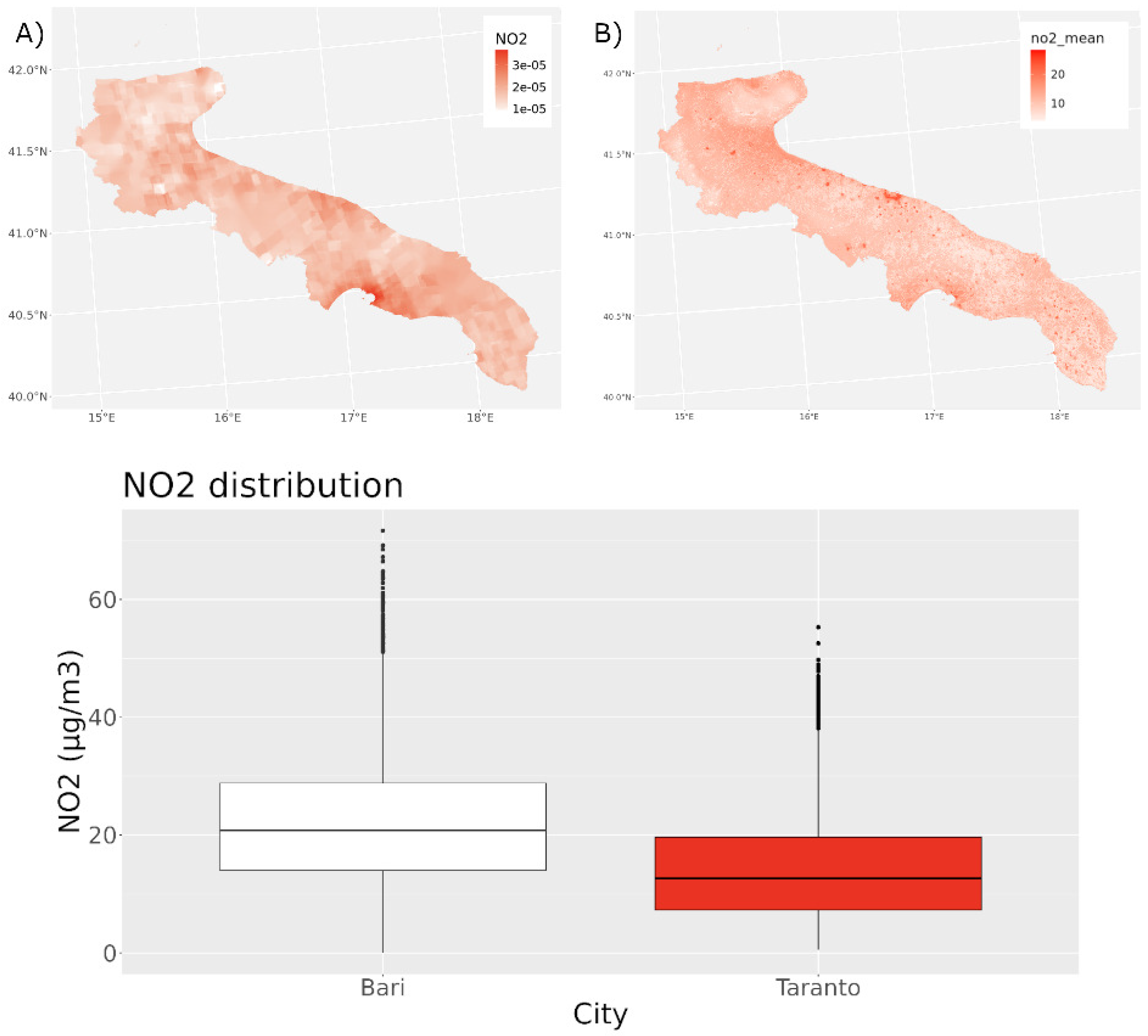
Figure 8 also highlights a key advantage of the proposed approach. Sentinel-5P tropospheric NO₂ mainly highlights large aggregated plumes (e.g., Taranto), whereas the model’s predicted surface NO₂ field captures much finer spatial gradients, including within Bari. When compared with ARPA ground measurements, both Bari and Taranto show elevated NO₂, but Bari exhibits even higher average concentrations despite the absence of a single dominant point source like the steel plant. This is consistent with population density data (Bari ≈ 2700 inhabitants/${\mathrm{k}\mathrm{m}}^2$ vs. Taranto ≈ 750 inhabitants/${\mathrm{k}\mathrm{m}}^2$) and intense traffic-related emissions. In other words, the model recovers both industrial and traffic-driven exposure patterns, which are not equally visible in the satellite column alone.

Temporal behavior (Figure 6), spatial distribution at 300 m (Figure 4 and Figure 7), and feature attribution via SHAP (Figure 5) together indicate that the model is not only fitting statistical structure, but is reproducing physically and chemically consistent patterns: winter NO₂ buildup under low wind; warm-season O₃ peaks driven by photochemistry; enhanced PM₁₀ near coastal/industrial zones tracked by AOD; and stronger spatial persistence of NO₂ hot spots across years compared to the more meteorology-driven O₃.

4. Discussion

4.1. Overall Performance and Comparison with Previous Studies

As shown in Table 5, the XGBoost model outperforms the linear model across all pollutants under random CV. This confirms that non-linear, interaction-aware models are required to fuse heterogeneous predictors (satellite columns, meteorology, AOD, land-use, and temporal harmonics) and to translate them into surface-level pollutant concentrations at 300 m resolution. The results are consistent with other studies in the literature. Stafoggia et al. achieved an average $R^2$ of 0.75 for daily predictions of PM₁₀ and PM_2.5 across Italy at ∼1 km resolution [68]. Our PM_2.5 and PM₁₀ $R^2$ values (0.67 and 0.64 in Table 5) are slightly lower, which is expected because we work at a finer spatial scale (300 m instead of ≥1 km), increasing spatial variability to be explained, and we rely on a smaller and regionally concentrated monitoring network within Apulia, rather than hundreds of stations nationwide. This resolution effect is well known: moving from kilometer to sub-kilometer grids sharpens intra-urban contrasts (traffic corridors, port areas, and industrial districts), which increases variance to be predicted and therefore mechanically lowers apparent $R^2$ at the pixel level. The performance of our model in predicting NO₂ and O₃ is also comparable to or better than values reported in the Italian literature. Silibello et al. report $R^2\approx 0.6$ for NO₂ and $R^2\approx 0.7$ for O₃ using hybrid modeling over the whole Italian territory at ∼1 km resolution [69]. In our case, random CV reaches $R^2=0.77$ for NO₂ and $0.78$ for O₃ (Table 5), again despite the more stringent (300 m) spatial resolution. This is notable because our study region is meteorologically complex (coastal recirculation, alternating land–sea breeze regimes, intense summer photochemistry) and industrially heterogeneous (steel, port logistics, traffic), which typically complicates surface pollutant modeling. The fact that the model maintains high skill in this setting suggests that even with fewer monitoring stations, high-resolution anthropogenic features (road density, port/industrial land-use, continuous urban fabric) and localized meteorology (WRF downscaled and resampled to 300 m) provide enough structure to generalize. When compared to studies outside Italy, our performance is broadly in line with machine learning air quality models developed in other complex regions. For example, Di et al. reported $R^2$ values in the 0.7–0.9 range for daily PM_2.5 across the continental United States at ∼1 km by combining satellite AOD, chemical transport model (CTM) output, land-use, and meteorology through an ensemble of statistical and machine learning learners [10]. Li et al. obtained $R^2$ values around 0.7–0.8 for PM_2.5 in China using deep ensemble approaches and rich station networks [11]. In Beijing and other megacities, deep recurrent models (LSTM, GRU, CNN-LSTM hybrids) used for PM_2.5 forecasting often report high predictive skill [7,8]; however, these studies typically operate in settings with dozens of stations within a single urban basin and do not always target sub-kilometer mapping of long-term exposure fields. Our framework, by contrast, is designed to deliver exposure fields at 300 m across an entire region that contains multiple distinct urban/industrial systems (Bari, Taranto, coastal logistics, rural inland). In this sense, our approach is closer to regional exposure mapping than to single-city forecasting, while retaining a spatial resolution that is comparable to neighborhood/block scale.

4.2. Public Health Relevance and Temporal Generalization

From a public health perspective, this point is non-trivial. Epidemiological and One Health studies increasingly focus on chronic exposure at the intra-urban scale (tens to hundreds of meters), because population vulnerability is not uniform within a city: residential areas sit next to major roads; schools and hospitals may lie downwind of ports or industrial stacks; and disadvantaged neighborhoods are often co-located with legacy industrial sources and high traffic loads. Our 300 m pollutant fields aim exactly at that scale. This is in line with recent air quality exposure work in North America and Northern Europe that emphasizes environmental justice and differential exposure, where within-city gradients are policy-relevant on their own and cannot be inferred from sparse fixed-site monitors alone [10,11]. As expected for data-driven models, LOYO CV exposes reduced daily performance due to year-to-year regime shifts, the limited number and uneven distribution of monitors, and the weaker seasonality and higher stochastic variability of PM. However, aggregating predictions to monthly and annual scales markedly improves $R^2$ (Table 6), supporting use for exposure assessment and One Health applications. In epidemiology and regulatory assessment, exposure is often averaged over months or years rather than interpreted day by day; our LOYO monthly $R^2$ values ($0.72$–$0.76$ for NO₂, O₃, and PM_2.5) indicate that such aggregated exposure fields are reliable even when an entire year is held out of training. This is important because it shows that the model is not just interpolating noise from individual days but is actually able to reconstruct the long-term spatial structure of exposure that matters for cardiovascular, respiratory, and neurodegenerative risk analyses [2,3,4].

4.3. Pollutant-Specific Atmospheric Interpretation

The differentiated behavior among pollutants has a clear atmospheric interpretation. NO₂ is a short-lived, primarily emitted pollutant tied to combustion (traffic, port activity, industrial stacks). Its spatial pattern is persistent in time (urban cores, road networks, industrial/harbor districts), and therefore NO₂ remains relatively robust in LOYO ($R^2=0.59$ daily). This agrees with prior work in Italy and across Europe, where NO₂ gradients are dominated by local emission intensity and street-scale dispersion [68,69]. In Apulia we observe the same structure: SHAP shows that NO₂ predictions increase sharply in areas with high road density, dense built-up fabric, and industrial land-use (Figure 5); wind speed carries strong negative SHAP values at high intensity, consistent with pollutant dilution. This supports a mechanistic reading: the model is not only “fitting” data, it is reconstructing physically interpretable source–dispersion relationships. PM₁₀ and PM_2.5 behave differently. Particulate matter in Apulia reflects both persistent sources (traffic, industry, port logistics, heating) and episodic inputs (resuspension, harbor/ship emissions, Saharan dust intrusions, stagnant meteorology). This mixture of steady and episodic drivers explains why daily LOYO skill is lower ($R^2=0.24$–$0.30$) than for NO₂, and why performance improves so strongly after temporal aggregation (up to $R^2$ = $0.79$ for annual PM_2.5). SHAP indicates that AOD is a dominant positive driver for both PM₁₀ and PM_2.5, while precipitation and stronger winds tend to suppress particulate levels (negative SHAP at high values). This is fully consistent with atmospheric physics: wet scavenging and ventilation remove particles, while dry, stagnant, high-AOD conditions favor accumulation. The spatial patterns we predict (Figure 4 and Figure 7) show PM₁₀ and PM_2.5 enhancements along coastal/industrial belts and port zones, including areas in Bari and Taranto with intense maritime and logistics activity. Similar harbor-related particulate enhancements have been described in other Mediterranean port cities, where ship emissions and bulk handling (e.g., minerals, coal, grain) locally elevate aerosol load [23,70].

4.4. Ozone-Specific Interpretation and Modeling Implications

O₃ represents the most conceptually challenging pollutant. Unlike NO₂ and primary PM, surface ozone is not directly emitted. It is formed photochemically from nitrogen oxides (${\mathrm{N}\mathrm{O}}_x$) and volatile organic compounds (VOCs) under sunlight and then shaped by transport, entrainment from the residual layer, $NO$ titration in traffic corridors, and boundary-layer dynamics. In coastal Mediterranean regions like Apulia, land–sea breeze circulations and recirculation cells can trap and re-inject aged air masses rich in photochemical products. This means that day-to-day O₃ fields depend strongly on meteorology and chemistry, and the surface O₃ level is not simply proportional to the instantaneous tropospheric O₃ column observed by Sentinel-5P. Indeed, previous studies have repeatedly emphasized that satellite tropospheric ozone columns correlate only weakly and inconsistently with surface ozone because they also integrate the free troposphere and large-scale background [14,71]. Our results are consistent with this view. In random CV, where the model is trained and tested within overlapping seasonal regimes, O₃ achieves $R^2=0.78$ (Table 5). Under LOYO, daily O₃ $R^2$ drops to $0.53$ (Table 6), highlighting that interannual variability in solar radiation, stagnation events, and photochemical regimes is difficult to extrapolate. Importantly, SHAP reveals that O₃ predictions are driven by temperature, emissivity (a proxy for surface energy balance and thus photochemical potential), and wind-related variables, with Sentinel-5P O₃ column still contributing positively in interaction with these drivers. That is, the column ozone on its own is not a good linear predictor, but in combination with meteorology and land-use it contains a usable signal. This is exactly the scientific motivation for applying non-linear ML instead of simple regression. From a modeling standpoint, this is also fully consistent with the theory of gradient boosting and modern feature selection: tree ensembles capture interactions and threshold effects without requiring large marginal correlations [57,58,65]. Consequently, correlation filtering is not an adequate criterion to discard features in non-linear pipelines; embedded methods and post hoc attributions (e.g., SHAP) are more appropriate to evaluate contextual usefulness [63,64,66,67]. The ozone result has two implications. First, it confirms that O₃ is intrinsically harder to generalize temporally than NO₂ or PM, which explains why O₃-health analyses often rely on multi-year averages or warm-season metrics rather than raw daily values. Second, it suggests clear directions for future improvement: adding explicit predictors of boundary-layer height, stagnation/recirculation indices, and VOC proxies (e.g., land-cover classes indicative of biogenic VOC emissions or industrial/port VOC sources) could capture more of the chemistry that drives O₃, especially in summer. This is aligned with recent calls in atmospheric modeling to hybridize physics and ML, using chemical transport model outputs as structured predictors while still letting data-driven methods learn residual structure [15,16].

4.5. Interpretability, Policy Relevance, and One Health Implications

SHAP analysis more broadly confirms that the model is physically consistent and therefore interpretable for policy. For NO₂, strong positive SHAP values are associated with dense built-up fabric, major roads, and industrial land-use; wind speed carries negative SHAP at high intensity, consistent with dispersion. For PM₁₀/PM_2.5, AOD is the top positive predictor, and precipitation/ventilation act as sinks. For O₃, temperature and emissivity (radiative forcing at the surface) play a central role, encoding the photochemical engine of ozone formation. This level of interpretability helps ensure that predicted maps can be discussed with air quality agencies and health stakeholders without treating the ML model as an opaque “black box”. Spatially, the 300 m maps (Figure 4 and Figure 7) and the comparison with ARPA measurements (Figure 8) highlight two important policy-relevant findings. First, NO₂ exposure in Apulia is not confined to a single point source (e.g., the Taranto steel complex) but also reaches high levels in dense urban/traffic environments like Bari, where population density and mobility are high. This means that industrial liability alone cannot explain the observed NO₂ burden: diffuse transport-related emissions in dense coastal cities can produce comparable or higher average exposure, as confirmed by ARPA station data. Second, PM₁₀ hotspots align with industrial/port and coastal areas, suggesting that harbors and shoreline logistics contribute to particulate exposure, not only classical industrial stacks. This supports targeted mitigation strategies (harbor electrification, dust suppression, and traffic control near port gates) that are already being discussed in several EU port cities. From a regulatory standpoint, these results are coherent with the 2024 EU Air Quality Directive, which explicitly encourages member states to combine monitoring networks with modeling and satellite data to generate high-resolution exposure assessments over populated areas, rather than simply multiplying fixed stations. Our framework directly responds to that directive: it fuses remote sensing, meteorology, and land-use to produce daily fields at 300 m, and it remains stable (especially after temporal aggregation) even when an entire year is withheld in training. This is relevant not only for compliance reporting but also for health impact assessment and One Health planning in regions where industrial activity coexists with densely populated urban waterfronts. We also underline the One Health dimension. Apulia is a densely inhabited coastal/industrial region where humans, ecosystems, and industrial pressures overlap on a relatively small spatial scale. Chronic exposure to NO₂, PM_2.5, and PM₁₀ is linked to respiratory and cardiovascular outcomes and, as emerging evidence suggests, to neurodegenerative processes [2,3,4]. Surface O₃, especially during warm-season peaks, exacerbates respiratory stress and can impair lung function. By reconstructing pollutant fields at 300 m resolution, including near schools, hospitals, and residential areas adjacent to industrial/port infrastructure, our model can directly support exposure analysis in a One Health framework, i.e., considering human health, environmental quality, and industrial/economic sustainability together.

4.6. Limitations and Future Work

Limitations remain. The ARPA network in Apulia, while compliant with regulations, is relatively sparse outside the main urban and industrial centers, which can introduce spatial bias and limit the model’s ability to learn fine-scale patterns in rural areas. O₃ remains challenging because satellite tropospheric O₃ columns integrate the entire free troposphere and are only indirectly sensitive to boundary-layer concentrations; this physical mismatch reduces temporal transferability. Interannual regime shifts in meteorology and emissions also reduce LOYO performance, especially at daily resolution. Future work should incorporate additional dynamical predictors (e.g., planetary boundary layer height, stagnation/recirculation metrics), explore hybrid physics–ML approaches that blend WRF/CTM outputs with data-driven learning [15,16], and include explicit uncertainty quantification to flag low-confidence conditions. We also expect that forthcoming missions such as NASA’s MAIA, designed to provide high-resolution particulate information, will further improve PM_2.5/PM₁₀ estimation and interpretation. Despite these challenges, our framework already demonstrates that high-resolution (300 m), explainable daily exposure maps for NO₂, PM₁₀, PM_2.5, and O₃ are feasible in a coastal industrial Mediterranean region. This is particularly relevant for One Health studies and environmental justice assessments in Bari, Taranto, and similar urban–industrial corridors, where both industrial plumes and traffic emissions matter and where vulnerable populations live close to sources.

5. Conclusions

In this work we developed an explainable machine learning framework to estimate daily surface concentrations of four key air pollutants (NO₂, O₃, PM₁₀, PM_2.5) across the Apulia region at 300 m resolution for the period 2019–2022. The model integrates Sentinel-5P column products, a calibrated multi-source AOD field, high-resolution meteorology from WRF, land-use and anthropogenic indicators (roads, buildings, industrial fabric, population), and temporal harmonics. We assessed predictive skill using both repeated random cross-validation and a Leave-One-Year-Out (LOYO) temporal validation scheme.

Random CV yielded high $R^2$ values (0.64–0.78 depending on pollutant), confirming that tree-based fusion (XGBoost) captures non-linear interactions between satellite, meteorological, and land-use drivers that linear models cannot. LOYO daily performance dropped, especially for $PM$ and O₃, reflecting interannual variability in atmospheric conditions and emissions. Crucially, however, after aggregation to monthly and annual means, the $R^2$ for NO₂, PM₁₀, PM_2.5, and partially also O₃ remained high (often $>0.7$), indicating that our maps are reliable for long-term exposure assessment at epidemiologically relevant time scales.

O₃ deserves special mention. Although O₃ achieved $R^2=0.78$ in random CV, its $R^2$ in LOYO daily prediction was lower ($0.53$), highlighting limited temporal transferability. This is consistent with the known physical mismatch between satellite tropospheric ozone columns and near-surface ozone and with the strong dependence of ozone on photochemistry, boundary-layer dynamics, and NO titration. Nevertheless, SHAP analysis shows that the model uses physically interpretable drivers (temperature, emissivity, wind, column O₃) to reproduce O₃ seasonality and warm-season peaks. This suggests that even ozone, which is traditionally difficult to downscale from satellite alone, can be partially constrained by a non-linear, explainable fusion framework.

From an application perspective, the generated maps resolve intra-urban gradients in Bari and Taranto, distinguishing traffic-related NO₂ exposure from industrial/harbor-related PM₁₀ loads. This level of spatial detail is directly relevant for health impact assessment, environmental monitoring, and targeted mitigation strategies in sensitive neighborhoods. The methodology therefore supports the goals of the 2024 EU Air Quality Directive, which encourages improved assessment (as opposed to simply multiplying monitoring stations) and aligns with future satellite missions such as NASA’s MAIA, which will provide high-resolution particulate measurements and is expected to further strengthen particulate matter estimation.

In summary, we provide what is, to our knowledge, the first daily, 300 m resolution, explainable AI-based air pollution product for Apulia, integrating satellite, meteorology, land-use and population indicators. The framework is transferable to other Mediterranean and coastal industrial regions with sparse monitoring networks and sets the stage for One Health and policy-relevant exposure studies focused on both chronic and acute pollution burdens.