Fusing Multi-Source Data with Machine Learning for Ship Emission Calculation in Inland Waterways

Abstract

Accurate estimation of ship emissions is essential for the effective enforcement of emission control policies in inland waterways. However, existing “bottom-up” models face significant challenges owing to severe data scarcity for inland ships, particularly regarding ship static parameters. This study proposes a novel data fusion and machine learning framework to address this issue. The methodology integrates real-time SO₂ and CO₂ pollutant concentrations on the Nanjing Dashengguan Yangtze River Bridge, Automatic Identification System (AIS) data, and meteorological information. To address the scarcity of design data for inland ships, web scraping was used to extract basic parameters, which were then used to train five machine learning models. Among them, the XGBoost model demonstrated superior performance in predicting the main engine rated power. A refined activity-based emission model combines these predicted parameters, ship operational profiles, and specific emission factors to calculate real-time emission source strengths. Furthermore, the model was validated against field measurements by comparing the calculated and measured emission source strengths from ships, demonstrating high predictive accuracy with R² values of 0.980 for SO₂ and 0.977 for CO₂, and MAPE below 13%. This framework provides a reliable and scalable approach for real-time emission monitoring and supports regulatory enforcement in inland waterways.

1. Introduction

The rapid development of the shipping industry has contributed to high-quality regional economic growth while simultaneously increasing air pollutant emissions from ships [1,2]. According to statistics, global ship emissions account for approximately 15% of total nitrogen oxides (NOx) and about 8% of total sulfur oxides (SOx) [3,4]. To mitigate shipping-related air pollution, the International Maritime Organization has designated Sulfur Emission Control Areas. Within these zones, particularly in inland river, ships are required to use marine fuel with a sulfur content of 0.1% or less [5,6]. The challenge of effectively calculating the emission source strength and monitoring the diffusion concentrations of SO₂ and other pollutants emitted by inland ships is a crucial task for maximizing the impact of inland river emission control areas [7,8,9].

Serving as the basis for studying maritime air pollution, ship emission calculation techniques have evolved from macro-scale estimation to increasingly refined models [10,11]. By combining information on ship types and emission factors for each fuel type, the total emissions of various pollutants are derived using “top-down” approaches. This approach is straightforward to calculate and is typically employed to develop emission inventories at a macro scale over extended time frames [12]. The widespread adoption of AIS information has led to the rise of the activity-based “bottom-up” method, which has now become the mainstream approach [13,14,15,16]. The core of the “bottom-up” methodology lies in its “micro-to-macro” approach. It begins with voyage activity data for individual ships, using precise algorithms to calculate emissions ship by ship, voyage by voyage, and hour by hour. These detailed results are subsequently aggregated to construct a regional or global emission inventory [17]. By adopting a “bottom-up” model for calculating ship emissions, it is possible to achieve a highly accurate quantification of emission source strength with superior temporal and spatial resolution [18,19]. Using inputs such as the power output, fuel consumption, and emission factors for a ship’s main engine, auxiliary engine, and boiler across various operational modes, the calculation results can more accurately reflect the ship’s emission intensity under its actual operating conditions [20]. Employing a “bottom-up” approach to construct ship emission models signifies a paradigm shift that extends far beyond merely “calculating a total emission quantity.” It transforms ship emissions from an ambiguous macro-level statistic into a clearly defined, dynamic, traceable, and analyzable target for micro-level management. This transformation has profound implications, enabling the accurate and effective management and control of ship-induced atmospheric pollution.

Within this framework, model accuracy is directly influenced by core design parameters: main engine power, auxiliary engine power, and design speed [21]. However, owing to the limited availability of such data, existing research typically relies on approaches such as retrieving data from classification society databases, administering questionnaires, establishing regression models, applying design standards, or using average values [22,23,24,25]. For instance, Huang et al. enhanced the traditional AIS-based ship emission model by incorporating corrections for wind, current, and wave effects on ships’ actual sailing speed [26,27]. The “bottom-up” approach is often employed to develop ship emission inventories for port areas. For seagoing ships, static parameters are typically well documented in classification society databases, and archival ship information can be obtained from port call data. However, inland ships suffer from severe data gaps in these databases. When calculating ship emissions, missing static parameters are primarily addressed through questionnaires and empirical methods, while regression-based predictions rely mainly on linear models, resulting in low forecasting accuracy. Thus, there is a pressing need to develop a real-time prediction method to estimate the engine power on in-service ships, enabling accurate real-time emissions calculations for ships underway [28].

The development of intelligent algorithms has driven the adoption of advanced techniques like machine learning and data fusion to tackle the challenges [29,30]. By synergistically merging multiple data sources, such as AIS data, meteorological conditions, and ship engineering parameters, these models can effectively capture the complex nonlinear relationships between a ship’s operational profile and its instantaneous emissions. A key advantage lies in their ability to impute missing static parameters (e.g., engine power) for data-scarce ships, moving beyond the limitations of simplistic linear regressions. Based on the above characteristics, machine learning-driven models can provide a robust and reliable tool for supporting precise environmental assessments [31,32].

Therefore, this study analyzed data on pollutant concentrations, AIS data, and wind direction and speed obtained from monitoring equipment installed on the Nanjing Dashengguan Yangtze River Bridge to investigate the spatiotemporal distribution of pollutant concentrations. Subsequently, to address the severe data scarcity issue for inland ships, web scraping techniques were employed to retrieve real-time ship parameters (including length, beam, gross tonnage, and ship type) based on Maritime Mobile Service Identify (MMSI) within the study area, enabling the prediction of power parameters and design speed. Following a comparative analysis of different machine learning prediction models, a “bottom-up” emission calculation model suitable for inland ships was developed by integrating emission factors. Finally, the proposed model is validated using field measurement data, and its performance is thoroughly evaluated and discussed.

2. Materials and Methods

2.1. Data Collection

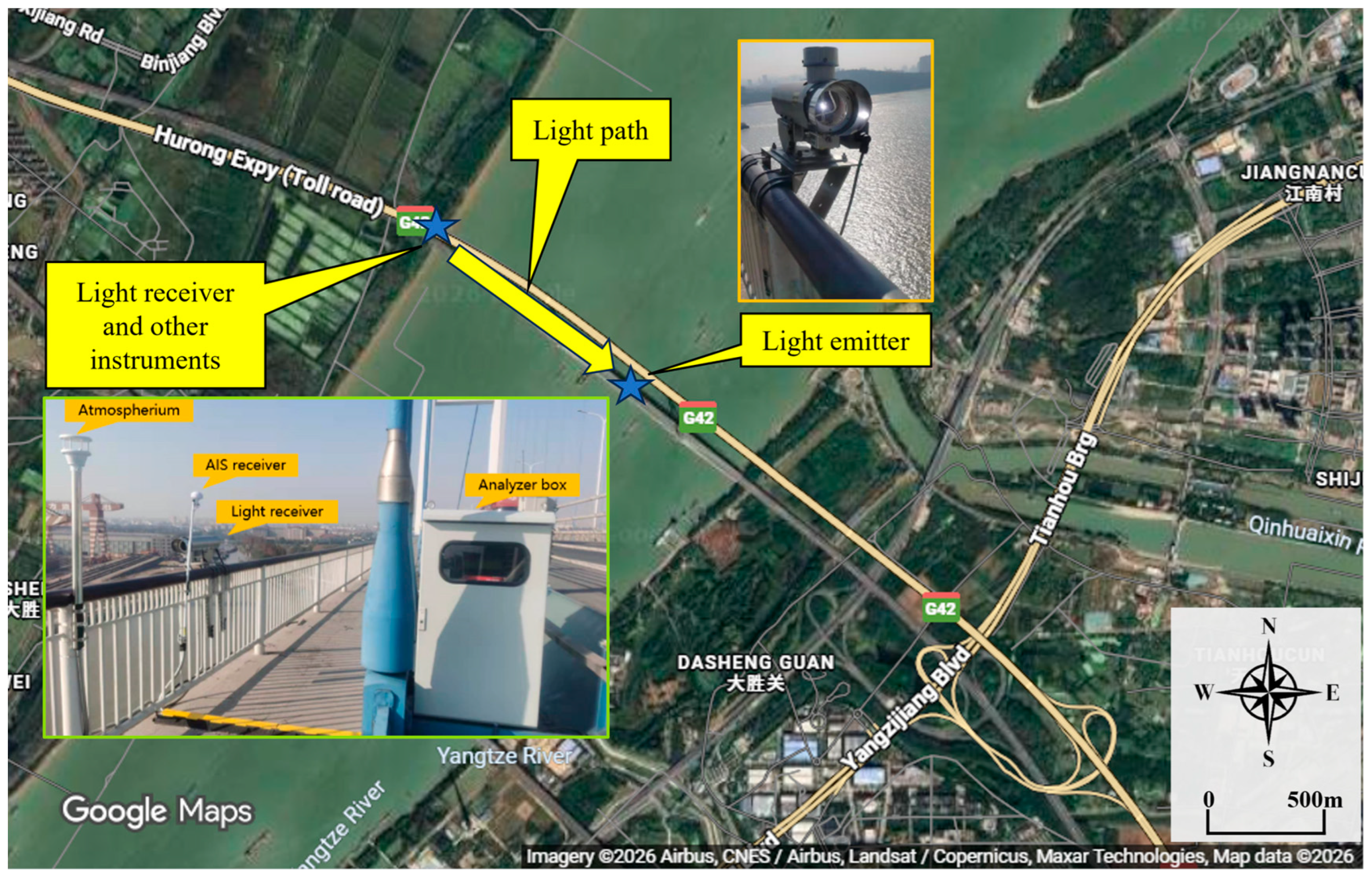
This study focuses on the inland waterway at the Nanjing Dashengguan Yangtze River Bridge, located in the Jiangsu section of the Yangtze River connecting Pukou District with Nanjing’s main urban area. In 2021, the research team deployed a spectroscopy-based remote sensing monitoring system in this study area, which was capable of collecting and monitoring real-time data on ship pollutant emission concentrations. The total optical path length of the system was approximately 350 m, providing sufficient monitoring coverage for upstream ships. As shown in Figure 1, the system comprises three components: an analytical unit, a light-emitting unit, and a light-receiving unit. A xenon lamp at the transmitter generated a light beam directed toward the detector, forming an unobstructed optical path. By evaluating the absorption characteristics of specific substances within the detected spectrum, the analytical unit enables the identification and quantitative analysis of the target pollutants.

Figure 1. Schematic diagram of equipment layout, position, and mode.

The data collected in this study included the following:

(1) Ship emission diffusion concentration data. Concentration data of SO₂ and CO₂ in ship exhaust were collected using a Differential Optical Absorption Spectroscopy (DOAS) system (OPSIS AB, Furulund, Sweden). The instrument identifies gas species based on the narrowband absorption characteristics of the gas molecules. This technique is capable of effectively detecting gaseous pollutants with characteristic absorption spectra (such as SO₂, NO₂, O₃, etc.), but has limitations in the direct quantitative detection of particulate matter (PM) due to its broad extinction spectrum and lack of specific absorption features. The DOAS is calibrated using certified SO₂ and CO₂ reference gases of known concentrations. This procedure verifies the linear response and detection sensitivity of the system and corrects for potential optical path drift or systematic errors.

(2) Ship AIS data. Ship data includes AIS and archival data. The AIS static data mainly comprises the ship’s name in Chinese and English, MMSI, and ship type. Real-time AIS dynamic data includes the ship’s latitude and longitude, navigation status, and speed. In addition, supplementary ship information, such as ship type, length, and beam, can be obtained from relevant ship information websites. Ship archival data covers basic ship records, company records, captain records, and accident archives. This study primarily focuses on basic ship archival data, including registration information, dimensional details, and onboard equipment parameters (e.g., main/auxiliary engine models and power ratings). Such archival data are mainly stored in major classification society databases. Python (v3.9.13), using the Requests library, was used to scrape archival ship information from websites. The collected data were organized and stored using the Pandas library.

(3) Meteorological data. For real-time, continuous monitoring of wind field variations, an anemometer and wind vane were employed. The instrument features a wind speed range up to 60 m/s and offers comprehensive 360-degree directional monitoring with high resolution and a ±3-degree precision. Wind speed and direction data were used for analyzing pollutant dispersion patterns, assisting in identifying the direction of local pollution sources, and providing a reference for background concentration correction in the subsequent sulfur content inversion based on the carbon balance method.

2.2. Data Preprocessing and Analysis

(1) AIS data preprocessing

To mitigate data issues from traffic density, human error, or system failures, preprocessing was indispensable. The procedure consisted of the following: (1) validity/format check. Records missing critical fields (e.g., MMSI, position, timestamp, speed) were discarded; (2) duplicate removal. Entries with identical MMSI, timestamp, and position were deleted to retain unique ship states; (3) outlier filtering. To ensure contextual plausibility, sailing speed was bounded between 0.5 knots (above drifting) and 30 knots (realistic maximum for this inland waterway), with violations removed; (4) missing data interpolation. Linear interpolation was applied to achieve a uniform temporal resolution of 1 s, facilitating subsequent computational steps.

The isolation forest algorithm was employed to handle anomalous data. The isolation forest is an unsupervised anomaly detection method for structured data that identifies samples that significantly deviate from the rest of the dataset. This algorithm offers low computational complexity because it does not rely on distance or density metrics or involve complex higher-order computations, enabling efficient execution even with large datasets. Based on the characteristics of anomalous data, the fundamental idea of the isolation forest is to iteratively split the data by randomly selecting a dimension for partitioning, dividing the current sample space into two subspaces, and repeating this process until each subspace contains only one data point. Dense clusters of data points require numerous splits, whereas outliers that deviate markedly from the majority are isolated quickly. Using this algorithm, data cleaning was performed for different ship types in this study. The model was configured with 100 isolation trees, an outlier fraction of 0.05, and two features, with other parameters set to their default values for model training. After data cleaning, 14,963 complete ship records were retained.

(2) Correlation analysis between ship emission dispersion concentrations and meteorological data

The influence of wind on exhaust dispersion can be summarized into two main aspects. First, wind direction determines the transport and migration of exhaust in the atmosphere; that is, the transport pathway of pollutants is directly related to wind direction. Understanding wind direction helps predict the potential areas of pollutant dispersion, facilitating the implementation of corresponding environmental protection measures. Second, wind speed affects the dispersion efficiency and spatial distribution of gas concentrations. Generally, higher wind speeds promote rapid pollutant dispersion, leading to quick dilution in the air and a consequent decrease in concentration. In contrast, at low wind speeds, pollutants move slowly through the atmosphere, leading to limited dispersion, high concentrations, and intensified local pollution.

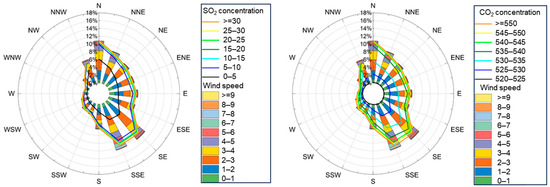
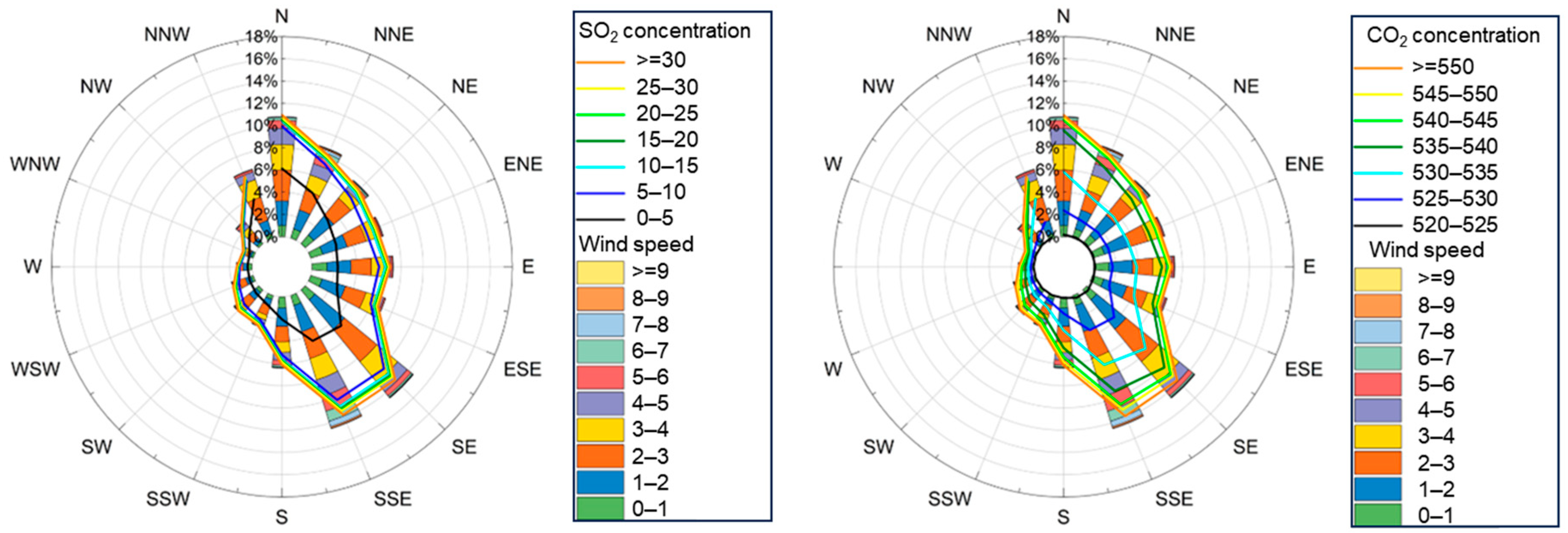
To further analyze the influence of wind direction and speed on exhaust dispersion concentrations, wind rose diagrams of SO₂ and CO₂ concentrations at the monitoring site were plotted (Figure 2). The correlations between dispersion concentrations and wind speed/direction, derived from Figure 2, can be summarized as follows: (1) The relationship between wind speed and dispersion concentration. High wind speeds enhance atmospheric turbulence, increasing the horizontal and vertical mixing of pollutants and thereby enhancing the transport efficiency of SO₂ and CO₂. Although strong winds facilitate the rapid dispersion and dilution of pollutants, the high emission intensity from sources such as ships can quickly transport a greater volume of pollutants to the monitoring site, resulting in elevated concentrations. This phenomenon indicates that, under the combined effects of high emission intensity and high wind speed, the transport distance of pollutants increases, while concentrations do not decrease significantly. In contrast, under low wind speeds, atmospheric mixing is limited, and the emitted pollutants may accumulate near the source, resulting in lower concentrations at the monitoring site. (2) The relationship between wind direction and dispersion concentration. Higher concentrations of SO₂ and CO₂ were observed under north-northwest (NNW) and north (N) winds, suggesting that pollution sources were likely located to the NNW or north of the monitoring site. Under these wind directions, pollutants were transported toward the monitoring point. Conversely, lower concentrations were recorded under east (E) and south (S) winds, which may be due to the absence of significant pollution sources in these directions or lower wind speeds, which reduce the efficiency of pollutant transport to the monitoring site. (3) The influence of meteorological conditions on dispersion concentration. Strong NNW and N winds were associated with higher pollutant concentrations and indicated more frequent ship activity or stronger emissions in these directions. Variations in wind direction and speed across different months may be related to seasonal meteorological changes, such as higher wind speeds and prevailing northerly winds in the spring. These variations affect the distribution and transport of atmospheric pollutants.

Figure 2. Wind rose diagrams of SO₂ and CO₂ concentrations at the monitoring site.

3. Ship Emission Calculation Model

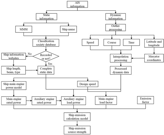
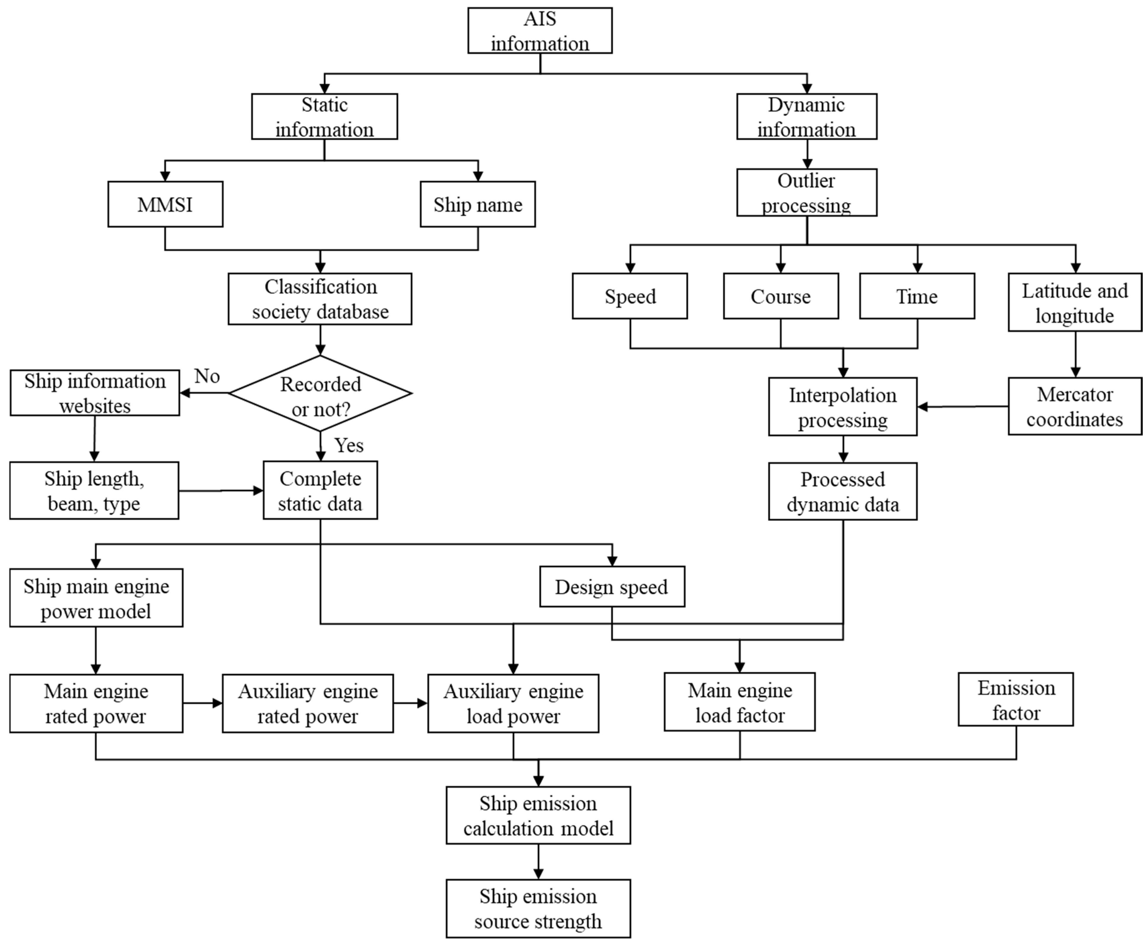
To address data scarcity for inland ships, this study proposes a method for determining ship design parameters. First, ship information is retrieved from the CCS and LR databases using the MMSI number and ship name from the AIS information. If data are missing, web scraping techniques are used to obtain basic ship parameters, including length, breadth, depth, gross tonnage, and ship type, from an online maritime platform using the MMSI number. These basic parameters are then used as input variables to estimate the main engine power, auxiliary engine power, and design speed. The main engine load factor is calculated from the actual and design speeds, while the auxiliary engine load factor is estimated based on the ship type and operating conditions. Using the supplemented static ship information and processed dynamic data, along with emission factors for inland ships, an activity-based emission calculation model is constructed to derive real-time emission source strengths. The flowchart of this process is shown in Figure 3.

Figure 3. Flowchart of the ship emission calculation model.

This study establishes a ship emission calculation model based on AIS information and fundamental ship data. The model parameters include the main engine rated power, auxiliary engine rated power, engine load factor, ship operating time, actual ship speed, design speed, and emission factors. The ship emission calculation model can be expressed as follows:

$$E_{i,j,k,l}={\sum }_{i=1}^n{P}_j\times L{F}_{j,l}\times T_{j,l}\times E{F}_{i,j}$$

where i denotes different pollutants (e.g., SO₂, NO_X, CO_2, etc.); j represents the engine type; l indicates the ship’s operating mode (including cruising, low-speed cruising, maneuvering, and berthing); E is the calculated emission amount (kg); P is the engine rated power (kW); LF is the engine load factor; T is the engine operating time (h); and EF is the emission factor for different pollutants (kg/kW·h).

(1) Ship type

Ships can be classified according to different criteria. Based on the purpose, ships can be categorized into cargo ships, passenger ships, tankers, and military ships. They may be divided by size into small, medium, large, and very large ships. Classification can also be based on deadweight tonnage or the type of propulsion system. In this study, ships are classified according to Lloyd’s Register of Shipping and previous studies and grouped into general cargo ships, bulk carriers, tankers, container ships, passenger ships, and other types [32,33]. By analyzing one day of AIS data from the Nanjing Dashengguan Yangtze River Bridge, it can be concluded that the most frequent ship type in the study area is the general cargo ship, accounting for 71% of the total, followed by bulk carriers at 15%. Tankers, container ships, and passenger ships account for approximately 5% of the total. These five ship types represent over 90% of the total, indicating that the classification method adopted in this study effectively covers most ships in the research area.

(2) Classification of ship operating modes

When a ship is cruising, accelerating, or decelerating, its engines operate under different conditions, resulting in different exhaust emissions. Therefore, it is necessary to calculate ship emissions for different operating modes. The study area is located along the Yangtze River in Nanjing, China. Because there are no port berths within the study area and ship traffic is high, the ship operating modes in the area can be classified, with reference to existing literature [27], into four categories: cruising, low-speed cruising, maneuvering, and berthing. The criteria for determining these modes are listed in Table 1.

Table 1. Classification of ship operating modes.

Operating Mode	Criteria
Cruising	sailing speed > 8 knots
Low-speed cruising	3 knots < sailing speed ≤ 8 knots
Maneuvering	1 knot < sailing speed ≤ 3 knots
Berthing	sailing speed ≤ 1 knot

3.1. Estimation Method for Ship Main Engine Power

For seagoing ships, static parameters are typically well-documented in classification society databases, and ship archival information can be obtained from port call data. However, inland ships suffer from severe data gaps in these databases. Therefore, regression models can be established using information such as ship length, beam, depth, ship type, and gross tonnage to fit the main engine power.

During the ship design process, the selection of the main engine should consider the design speed, propeller efficiency, fuel consumption, principal dimensions such as length, beam, and draft, as well as economic efficiency and operational performance. The Admiralty coefficient method is the most commonly used simplified approach for selecting the main engine. Its fundamental principle is that when the principal dimensions, hull form coefficients, design speed, and other parameters of the designed ship are similar to those of a parent ship, the parent ship’s Admiralty coefficient can be used to estimate the required main engine power [31,32]:

$$P_M={\displaystyle \frac{{∆}^{\frac{2}{3}}{V}_m^3}{C}}$$

where $P_M$ represents the main engine power of the ship (kW); C is the Admiralty coefficient; $V_m$ is the design speed (knot); and $∆$ denotes the design displacement (t). $∆$ can be calculated as follows:

$$∆=1.025L_{pp}B{T}_s{C}_b$$

where 1.025 is the seawater density (t/m³); $L_{pp}$ is the length between perpendiculars (m); B is the beam (m); $T_s$ is the design draft (m); and $C_b$ is the block coefficient. By approximating the length between perpendiculars as the overall ship length L and disregarding the design draft, the relationship between main engine power and the length and beam of ships can be derived as follows. The main engine power of a ship exhibits a close correlation with the product of its length and beam.

$$P_M~L\times B$$

To optimize the prediction of ship main engine power, machine learning models such as Decision Tree Regression (DTR), Random Forest Regression (RFR), Gradient Boosting Regression (GBR), eXtreme Gradient Boosting (XGBoost), and Light Gradient Boosting Machine (Light GBM) were selected to establish a method for estimating the rated power of ship main engines. A comparative analysis of the fitting performance of these models was subsequently conducted.

The DTR model is a fundamental regression technique. Its basic idea is to recursively partition the input dataset [34]. The main steps are as follows: (1) select a feature as the root node and split the data into two subsets; (2) repeat step 1 for each subset, continually dividing the dataset into smaller subsets until a stopping criterion is met, at which point recursion halts and the subset becomes a leaf node; (3) at each leaf node, compute the mean or median of the sample data as the predicted value for that leaf. The advantages of the DTR model include its ability to handle nonlinear relationships and high-dimensional data. Its drawbacks include sensitivity to data noise, which can lead to unstable results and overfitting.

The RFR model is an improvement over the DTR. It employs bootstrap sampling to randomly draw multiple subsets from the training set, with each subset used to train a separate decision tree. During prediction, the results from all decision trees are aggregated to produce the final prediction. The advantages of RFR include reduced overfitting compared to single decision trees and lower sensitivity to data noise. Its disadvantages include difficulty in interpreting the model’s specific decisions and relatively slower training speed [35,36].

The GBR model iteratively combines multiple decision trees to improve overall predictive performance progressively [37]. The core of the algorithm lies in minimizing the loss function using gradient descent while employing decision trees for prediction. For complex datasets, GBR can improve predictive performance by increasing the number of decision trees, but in high dimensions, it may suffer from the curse of dimensionality. Tuning parameters is therefore necessary to avoid overfitting and underfitting.

XGBoost is a machine learning algorithm improved upon GBR. Building on GBR, it incorporates optimization techniques such as second-order Taylor expansions, regularization, and parallel computing, thereby improving both the model’s accuracy and efficiency. In the XGBoost regression algorithm, each decision tree serves as a weak learner, and multiple trees are iteratively trained to improve overall predictive performance gradually. To prevent overfitting, XGBoost introduces a regularization term that limits model complexity and improves generalization. The advantages of the XGBoost regression algorithm include high efficiency, accuracy, and scalability. In addition, model complexity can be controlled by tuning hyperparameters to avoid overfitting or underfitting, while parallel computing can accelerate training [38,39].

Light GBM is also an algorithm improved upon GBR, but it differs in its implementation and performance optimization. First, the tree-splitting strategy differs: traditional GBR adopts a greedy approach that selects the optimal feature and split point to maximize the reduction in the loss function; whereas Light GBM adopts a leaf-wise growth strategy that splits the leaf with the largest gain, thereby reducing tree depth and increasing training speed. Second, the feature selection method differs: traditional GBR uses a greedy algorithm, which may overlook useful features and degrade prediction accuracy. Lastly, the split-point selection differs: in traditional GBR, continuous features must be sorted and all possible split points enumerated to select the optimal one. This process consumes considerable time and memory, especially on large-scale datasets [40,41].

During model training, all sample data were randomly split into a training set and a test set with a ratio of 7:3. To optimize the XGBoost model’s predictive performance, hyperparameter tuning was performed using Grid Search combined with 5-fold cross-validation. Key hyperparameters tuned included: learning rate (range: 0.01–0.3), maximum tree depth (range: 3–10), subsample ratio for training each tree (range: 0.6–1.0), and the regularization parameter (reg_lambda). The final model was trained with the following optimal parameter set: learning_rate = 0.1, max_depth = 6, subsample = 0.8, reg_lambda = 1. A similar tuning process was applied to the other models (DTR, RFR, GBR, Light GBM) to ensure a fair comparison.

3.2. Determination of Other Parameters

(1) Engine load factor

Engine load factor measures the actual load level of a ship’s main engine during operation. The load factor of the auxiliary engine is closely linked to ship type and sailing speed, as detailed in Table 2 [31,32].

Table 2. Auxiliary engine loading under differing ship types and operating modes.

Ship Type	Cruising	Low-Speed Cruising	Maneuvering	Berthing
General cargo ship	0.17	0.27	0.45	0.22
Bulk carrier	0.17	0.27	0.45	0.22
Tanker	0.13	0.27	0.45	0.67
Container ship	0.13	0.25	0.50	0.17
Passenger ship	0.80	0.80	0.80	0.64
Other ship type	0.17	0.27	0.45	0.22

It is recognized that emission calculation accuracy is highest when using load factors and fuel flow rates obtained directly from shipboard systems. However, the acquisition of real-time engine performance data across diverse ships presents significant challenges related to data availability and system interoperability. Due to these impediments, direct measurement is not applicable within the framework of this analysis. This research therefore adopts the conventional speed-load proportionality principle—whereby the load factor is estimated by cubing the ratio of actual to design speed—a method consistently employed in authoritative regional and port-level emission studies. This established approximation provides a validated basis for estimating emissions in data-scarce scenarios [42,43]:

$$LF={\left({\displaystyle \frac{V_a}{V_m}}\right)}^3$$

where $V_a$ represents the ship’s actual sailing speed, obtainable from AIS data (knots); $V_m$ represents the ship’s design speed or maximum speed (knots), which is typified by the following averages: 15 knots for cargo-bulk carrier and cargo-oil tanker, 21 knots for cargo-container and passenger, and 15 knots for remaining categories [43]. In addition, the auxiliary engine load power can be estimated based on the ship type and the main engine rated power, with the corresponding values provided in Table 3 [31,32].

Table 3. Power ratio between auxiliary engine and main engine for different ship types.

Ship Type	Auxiliary to Main Engine Power Ratios
General cargo ship	0.191
Bulk carrier	0.222
Tanker	0.211
Container ship	0.220
Passenger ship	0.278
Other ship type	0.269

(2) Emission factors

The emission factors of ship exhaust pollutants are directly related to engine type, fuel type, and fuel sulfur content. Xu et al. researched atmospheric pollutant emissions from inland ships in Jiangsu Province, China. The results indicate that the main engines for inland ships primarily use medium-speed engines, while auxiliary engines generally employ high-speed diesel engines. Furthermore, the emission factors of ships are significantly influenced by fuel quality. Different fuel sulfur contents correspond to different emission factors, which can be adjusted using fuel correction factors [44,45]. The corrected ship emission factors are presented in Table 4. Emission factors for sulfur content not listed in the table can be obtained using linear interpolation.

Table 4. Ship emission factor for different pollutants (g/kW·h).

Engine Type	Pollutant	Sulfur Content	High-Speed Engine		Medium-Speed Engine		Low-Speed Engine
			Seagoing Ship	Inland Ship	Seagoing Ship	Inland Ship	Seagoing Ship	Inland Ship
Main engine	SO2	1.5%	10.30	5.77	11.31	6.33	11.31	6.33
		0.5%	3.43	1.92	3.77	2.12	3.77	2.12
		0.2%	1.37	0.77	1.51	0.84	1.51	0.84
		$\le$0.1%	0.69	0.38	0.75	0.42	0.75	0.42
	NOX	1.5%	18.10	16.29	14.00	12.60	12.70	11.43
		0.5%	18.90	17.01	14.62	13.16	13.26	11.94
		0.2%	18.90	17.01	14.62	13.16	13.26	11.94
		$\le$0.1%	18.90	17.01	14.62	13.16	13.26	11.94
	CO2	1.5%	620.00	620.00	680.00	680.00	680.00	680.00
		0.5%	620.00	620.00	680.00	680.00	680.00	680.00
		0.2%	620.00	620.00	680.00	680.00	680.00	680.00
		$\le$0.1%	620.00	620.00	680.00	680.00	680.00	680.00
Auxiliary engine	SO2	1.5%	6.33	6.33	NA		NA
		0.5%	2.12	2.12
		0.2%	0.84	0.84
		$\le$0.1%	0.42	0.42
	NOX	1.5%	11.49	11.49	NA		NA
		0.5%	12.00	12.00
		0.2%	12.00	12.00
		$\le$0.1%	12.00	12.00
	CO2	1.5%	690.00	690.00	NA		NA
		0.5%	690.00	690.00
		0.2%	690.00	690.00
		$\le$0.1%	690.00	690.00

Note: Engines with a rotational speed exceeding 1400 rpm are classified as high-speed engines; those with speeds between 130 rpm and 1400 rpm are defined as medium-speed engines; and engines operating below 130 rpm are categorized as low-speed engines [44].

It should be noted that due to the scarcity of publicly available auxiliary engine power data for inland ships, an independent predictive model was not developed; instead, empirical ratios from literature were used. Similarly, the auxiliary engine load factors are typical averages for ship types and modes, not accounting for individual ship variations. The main engine load model, while dynamic, is based on a simplified cubic speed relationship. These represent practical simplifications given current data constraints but introduce uncertainties that future studies with more extensive measurements could address.

4. Results Analysis

4.1. Ship Main Engine Power

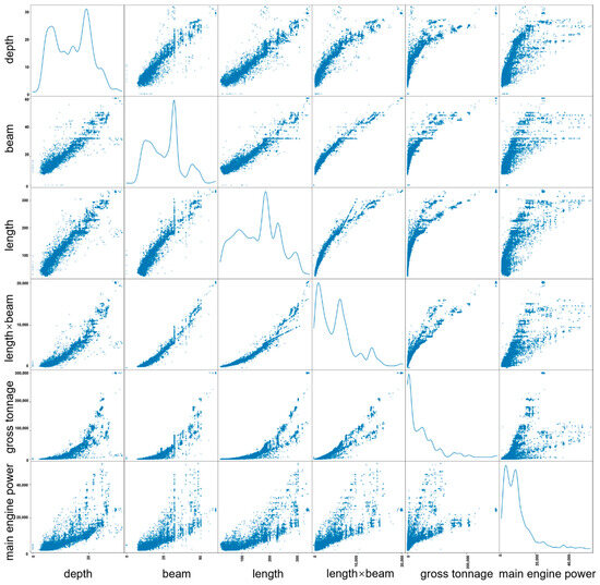
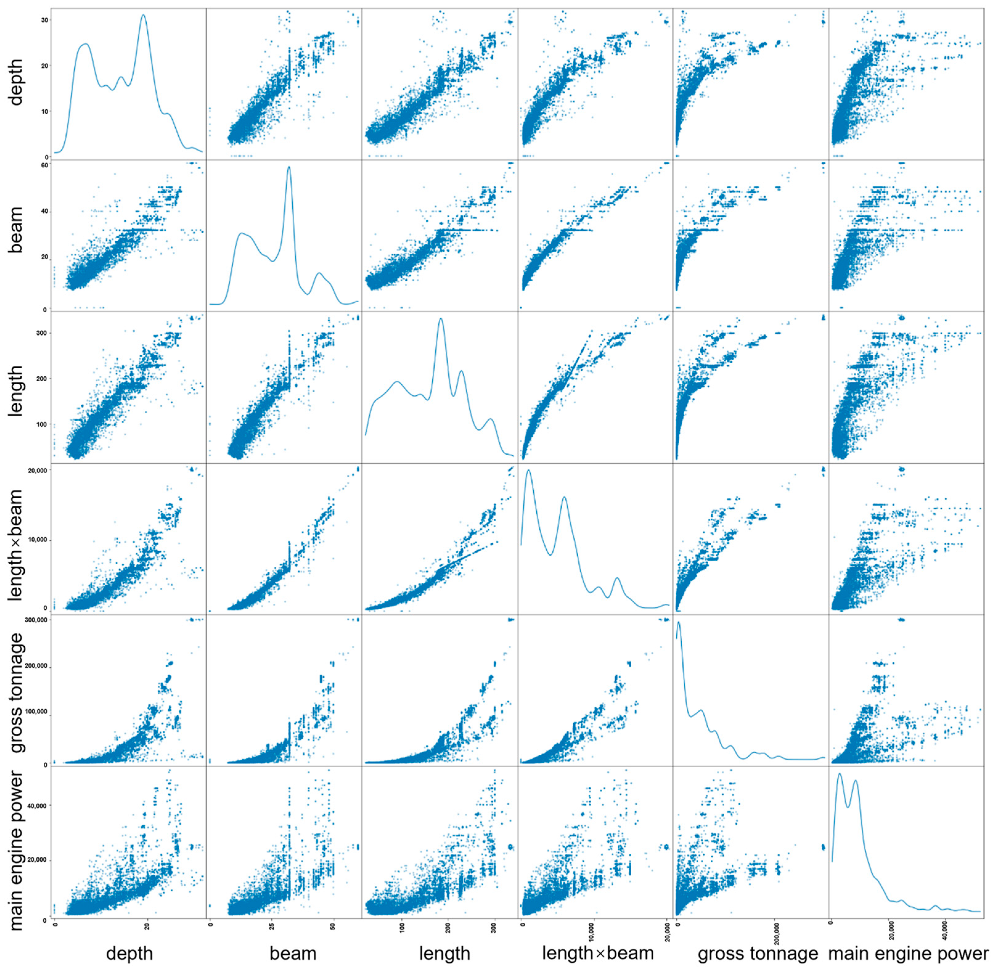
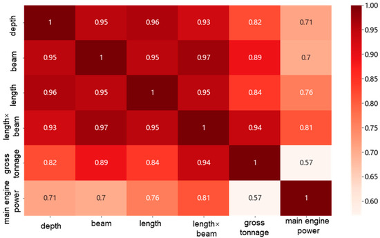
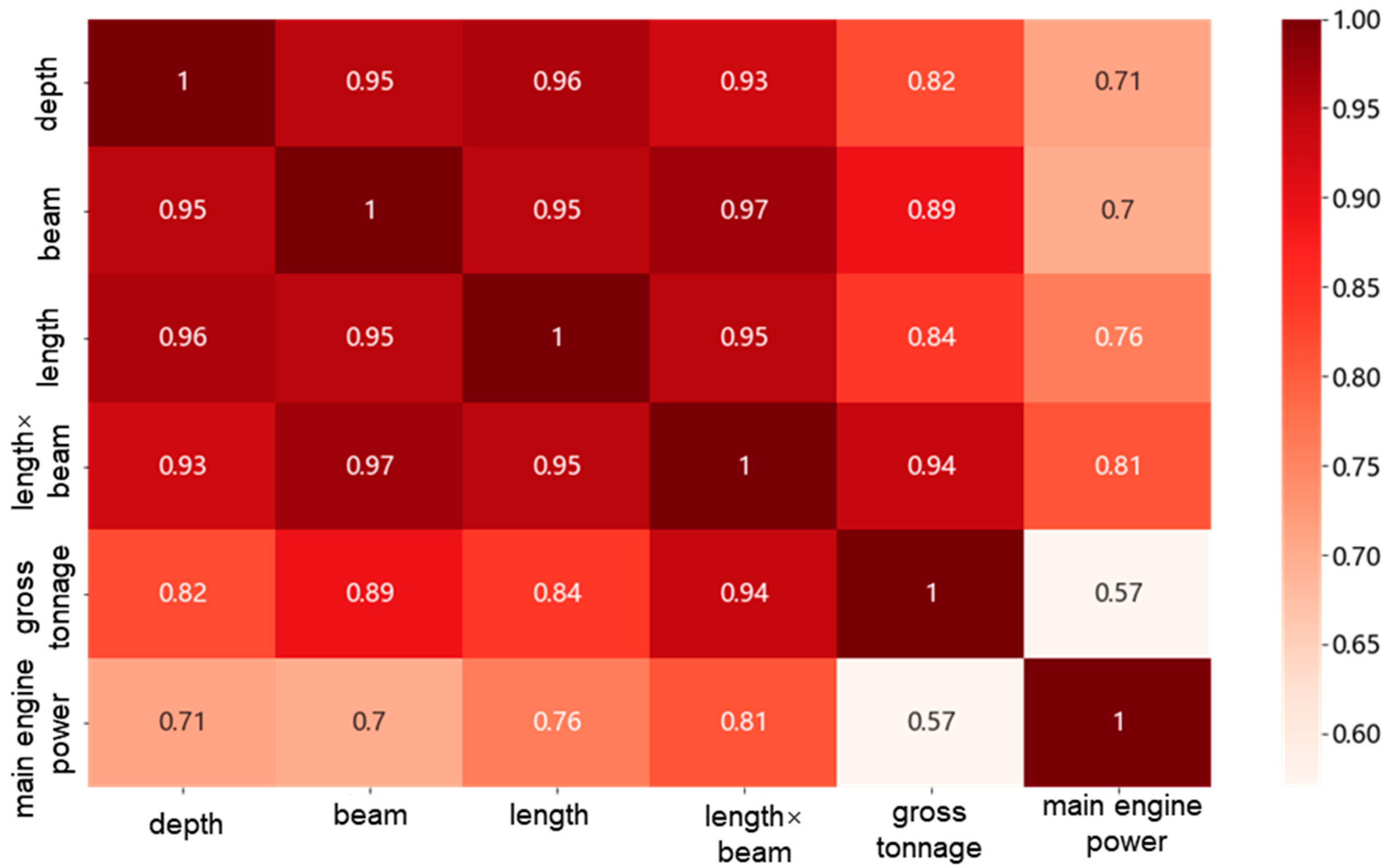
Parameters including ship length, beam, depth, the product of length and beam, gross tonnage, and main engine power were selected from the complete ship dataset. Scatter plots and correlation analyses were performed for each feature pair, and the results are presented in Figure 4. The scatter plots reveal that depth, length, beam, and the product of length and beam all exhibit certain correlations with main engine power. In contrast, gross tonnage shows no significant correlation with main engine power. Further analysis of the correlation heatmap (Figure 5) indicates that the main engine power has the highest correlation with the product of ship length and beam. Given concerns about multicollinearity, a linear regression model for predicting main engine power was established using the product of ship length and beam.

Figure 4. Scatter plot matrix of ship main engine power.

Figure 5. Correlation coefficient matrix of ship main engine power.

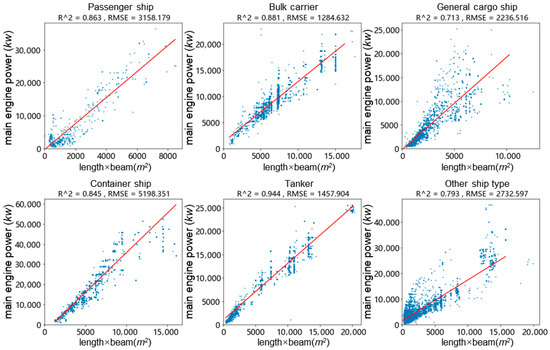
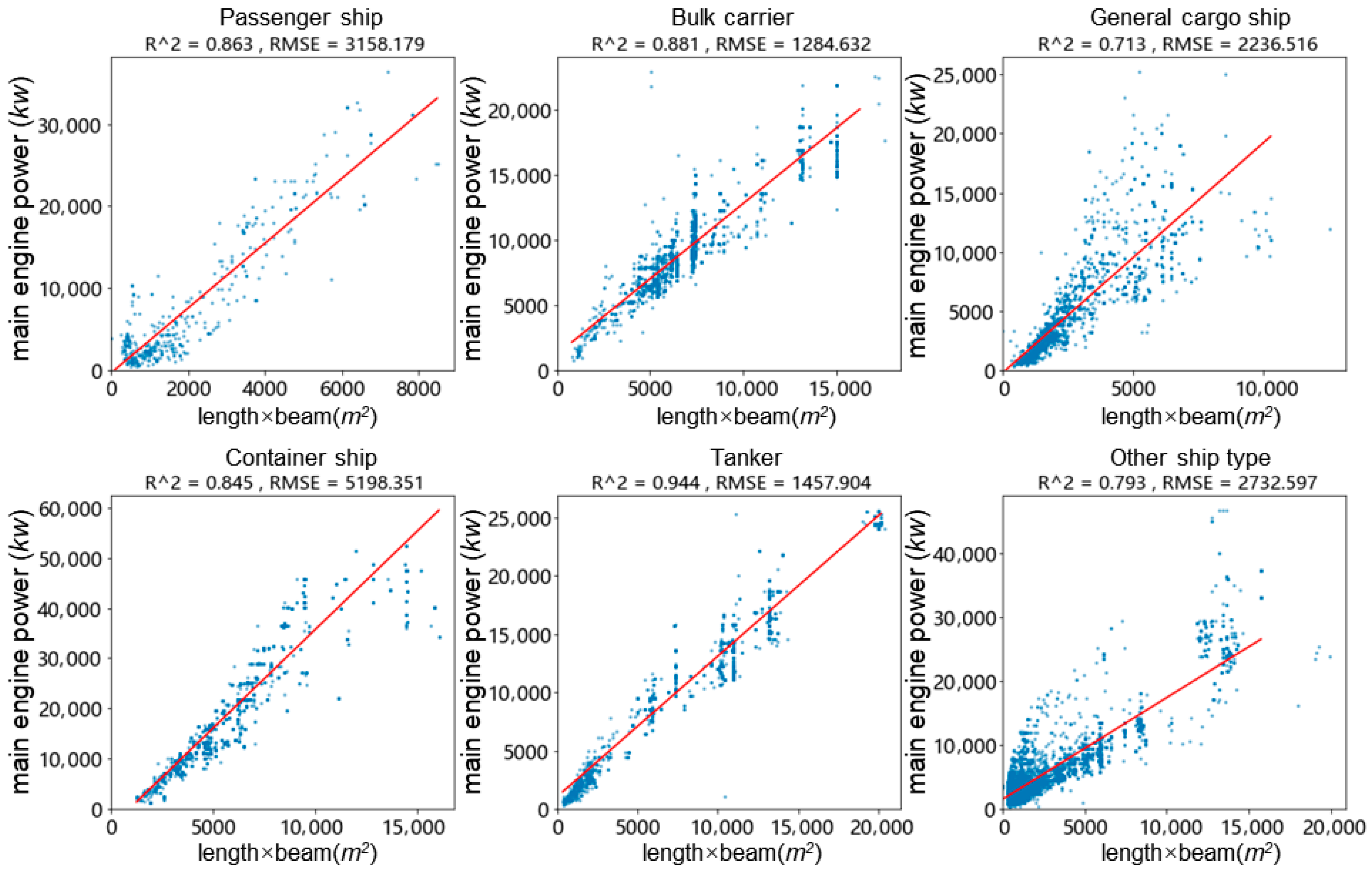
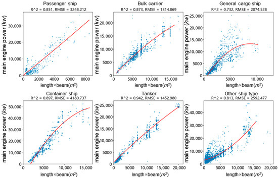
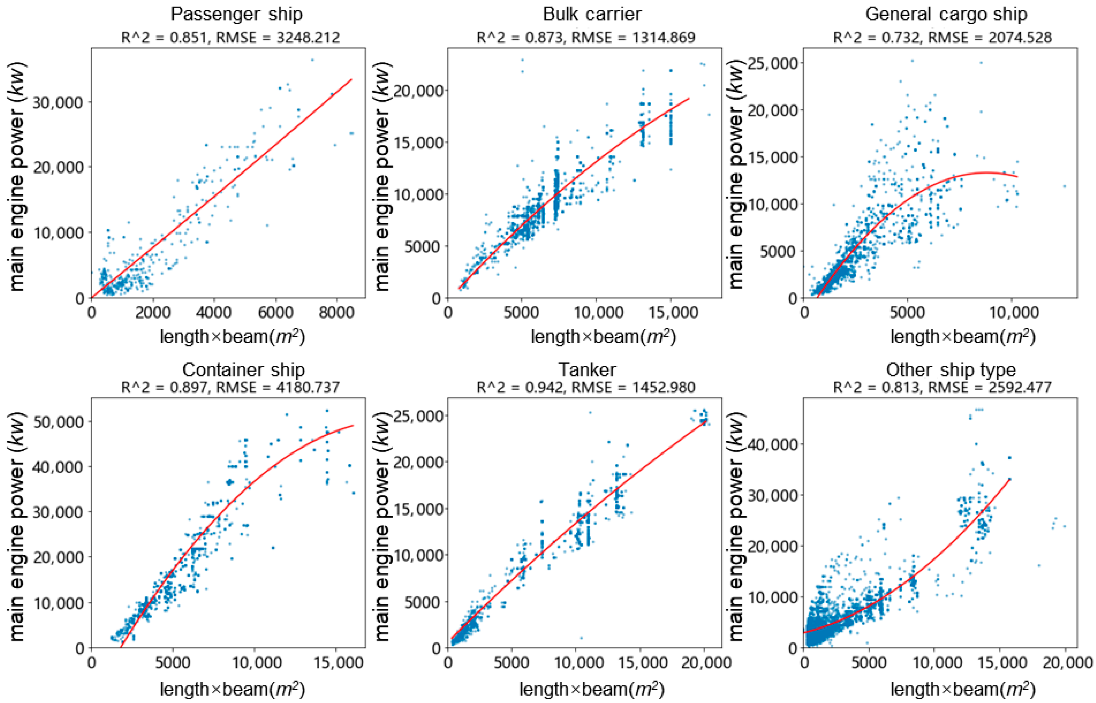
From the scatter plot distributions and correlation coefficient heatmap presented above, a clear positive correlation can be observed between the product of ship length and beam and the main engine power. A polynomial regression approach was therefore adopted for fitting. Model training was conducted using Python (v3.9.13) and the Scikit-learn (Sklearn) library. When the degree d = 1, corresponding to a linear regression model, the fitting performance is illustrated in Figure 6. The figure shows that tankers achieved the best fit, with an R² of 0.944, while general cargo ships exhibited a moderate fit with an R² of 0.713. The likely reason for this discrepancy is that the classification of general cargo ships is relatively broad, encompassing many sub-types and a larger number of ships within the dataset. In contrast, tankers have fewer subcategories and a more concentrated distribution of data. When d = 2, a quadratic polynomial regression was applied to the data, with the resulting fit shown in Figure 7. It can be observed that the R² values for passenger ships, bulk carriers, and tankers remained largely unchanged, whereas those for general cargo ships, container ships, and other ship types improved. As the degree d increases further, the R² value improves slightly but not significantly.

Figure 6. Scatter distributions and fitted curves for each ship type (d = 1).

Figure 7. Scatter distributions and fitted curves for each ship type (d = 2).

A significance test and fitting performance analysis were conducted for the quadratic polynomial regression models of main engine power across different ship types. The evaluation metrics employed were the Root Mean Squared Error (RMSE) and the Mean Absolute Percentage Error (MAPE). As shown in Table 5, the p-values for the quadratic polynomial regression models of all ship types were less than 0.05, indicating that the regression equations are statistically significant. However, based on RMSE and MAPE, the models’ fitting performance is generally unsatisfactory. Apart from bulk carriers and tankers, which show errors around 10% and 15%, respectively, the errors for other ship types are notably high. This suggests the need to consider alternative prediction models and incorporate additional independent variables.

Table 5. Significance testing and goodness-of-fit analysis (d = 2).

Ship Type	R-Squared	p-Value	RMSE	MAPE (%)
Passenger ship	0.851	<0.001	3248.212	67.511
Bulk carrier	0.873	<0.001	1314.869	10.170
General cargo ship	0.732	<0.001	2074.528	30.339
Container ship	0.897	<0.001	4180.737	22.403
Tanker	0.942	<0.001	1452.980	15.151
Other ship type	0.813	<0.001	2592.477	38.680

Using the Scikit-learn library in Python, five machine learning models including DTR, RFR, GBR, XGBoost, and Light GBM were employed to establish regression prediction methods for different ship types. The ship length, beam, and the product of length and beam were used as input variables, with the rated main engine power as the target variable. The prediction results were compared with those of the linear regression model, as shown in Table 6. The XGBoost regression model consistently outperforms the linear regression model across all ship types. Specifically, bulk carriers, tankers, and container ships achieved the best prediction accuracy, with errors controlled within 10%. In contrast, the predictive performance for passenger ships and other ship types was moderate, with MAPE values of 36.1% and 26.9%, respectively. The likely reason is that the classification of passenger ship and “other ship type” is relatively broad. However, as indicated by earlier statistics, passenger ships represent a very small proportion (less than 1%) of the ship types in the study area. In contrast, the “other ship types” category comprises a variety of sub-types. Further subdivision would not only lead to an excessive number of ship categories but also result in insufficient sample data for each type to support robust modeling. Moreover, obtaining accurate auxiliary engine power and load coefficients for more finely divided ship types would be challenging. Given the study’s feasibility and the practicality of engineering applications, the current ship classification method is retained in this research.

Table 6. Comparison of prediction performance for different models and various ship types.

Ship Type	Regression Model	RMSE	MAPE (%)
Passenger ship	Linear Regression	3119.7738	60.4224
	DTR	3075.4691	51.4441
	RFR	2909.5611	52.0529
	GBR	3024.4207	36.9852
	XGBoost	3104.6079	36.1128
	Light GBM	2950.0646	40.1239
Bulk carrier	Linear Regression	1245.1242	10.4243
	DTR	1209.2986	11.0203
	RFR	1136.7156	10.4094
	GBR	975.7377	7.3534
	XGBoost	957.6757	6.9676
	Light GBM	992.8094	7.6061
General cargo ship	Linear Regression	2042.3197	31.2424
	DTR	1980.488	27.6039
	RFR	1902.9098	26.3724
	GBR	1510.9006	19.857
	XGBoost	1472.4682	17.6716
	Light GBM	1578.2153	20.4873
Container ship	Linear Regression	3681.8772	18.4171
	DTR	3181.1624	16.7206
	RFR	2981.3452	15.4678
	GBR	1894.8023	8.6646
	XGBoost	1752.9091	6.4317
	Light GBM	2055.1868	9.3213
Tanker	Linear Regression	1311.2026	11.935
	DTR	1274.7853	15.1042
	RFR	1205.8273	13.973
	GBR	1013.5477	9.1181
	XGBoost	991.3893	8.4704
	Light GBM	1009.219	9.1754
Other ship type	Linear Regression	2608.9524	37.8055
	DTR	2293.505	36.0986
	RFR	2214.8929	35.2708
	GBR	1988.7106	28.6823
	XGBoost	1988.2887	26.9075
	Light GBM	2007.8156	28.835

4.2. Example Calculation of Ship Emission Source Strength

As shown in Table 4, ship emission factors are significantly influenced by fuel quality, with different sulfur contents corresponding to different emission factors [44,45]. Therefore, determining the sulfur content of ship fuel is a prerequisite for calculating the emission source strength. Fuel sulfur content refers to the mass percentage of sulfur in the fuel. It is a key parameter determining the SO₂ concentration in ship exhaust and a core regulatory indicator in emission control area regulations, such as the 0.1% limit. Among the methods for determining ship fuel sulfur content, the carbon balance approach is a commonly adopted rationale. It involves simultaneously measuring the concentrations of SO₂ and CO₂ and inferring the fuel sulfur content based on their concentration ratio [31,46]. For the specific calculation, it is first necessary to isolate the actual contribution of ship emissions from the monitored total concentration. The bridge-mounted DOAS system obtains the monitored concentrations of SO₂ and CO₂, denoted as $C_{{SO}_2}$ and $C_{C{O}_2}$, when a ship passes through the monitoring cross-section. This concentration is the superposition of the ambient background concentration $C_{background}$ and the diffusion concentration from ship emissions. By analyzing the ship’s trajectory and the concentration time series, a stable average concentration from a period sufficiently upstream or after the ship’s influence is selected as the background value, thereby isolating the concentration increment caused by the ship’s emissions:

$$∆C_{{SO}_2}=C_{{SO}_2}-C_{background,{SO}_2}$$

$$∆C_{{CO}_2}=C_{C{O}_2}-C_{background,{CO}_2}$$

The derived diffusion concentrations of ship emissions, $∆C_{{SO}_2}$ and $∆C_{{CO}_2}$, are then substituted into the carbon balance equation, and the fuel sulfur content can be expressed as

$$S={\displaystyle \frac{∆C_{{SO}_2}\times 32}{{∆C}_{{CO}_2}\times 12}}\times 87\%$$

where 32 and 12 are the molar masses of SO₂ and CO₂ (g/mol), respectively; 87% represents a typical value for the mass fraction of carbon in fuel oil. This method directly establishes a quantitative relationship between the monitored concentrations and fuel properties. The calculated sulfur content serves as a key input for determining the corresponding emission factors for SO₂ and CO₂ from Table 4. This provides a reliable basis for the subsequent “bottom-up” calculation of emission source strength and directly supports real-time screening of ship fuel compliance.

To specifically illustrate the calculation procedure of the above method, an inland ship passing through the monitoring cross-section of the Nanjing Dashengguan Yangtze River Bridge is taken as an example to demonstrate the complete calculation process from pollutant concentrations to ship emission source strength.

(1) Given conditions

The DOAS system measured peak diffusion concentrations (after background subtraction) of SO₂ and CO₂ in the ship’s exhaust as $∆C_{{SO}_2}$ = 20 ppm and $∆C_{{CO}_2}$ = 1.5%. AIS data indicate that the ship is a general cargo ship with an actual speed $V_a$ = 8.5 knots. Basic parameters obtained via web scraping are: length $L$ = 65 m, beam $B$ = 12 m. Meteorological conditions over the water area remained stable, with light winds. The design speed of the ship is taken as $V_m$ = 15 knots (a typical value for general cargo ships). Based on the sailing speed and the criteria in Table 1, the ship is determined to be in the cruising mode.

(2) Calculation steps

Step 1: Calculate fuel sulfur content

The fuel sulfur content S is calculated from the monitored concentrations using the carbon balance method:

$$S={\displaystyle \frac{∆C_{{SO}_2}\times 32}{∆C_{{CO}_2}\times 12}}\times 87\%={\displaystyle \frac{\left(20/\mathrm{10,000}\right)\times 32}{1.5\times 12}}\times 0.87\approx 0.00309=0.309\%$$

The calculated fuel sulfur content is approximately 0.309%. This value is used to determine the SO₂ and CO₂ emission factors for the main and auxiliary engines.

Step 2: Determine emission factors

Main engine emission factors. Assuming the main engine of this general cargo ship is a medium-speed diesel (the predominant type). Linear interpolation from Table 4 yields a SO₂ emission factor of 1.30 g/kW·h and a CO₂ emission factor of 680.00 g/kW·h.

Auxiliary engine emission factors. The auxiliary engine is typically a high-speed diesel. Linear interpolation from Table 4 yields a SO₂ emission factor of 1.30 g/kW·h and a CO₂ emission factor of 690.00 g/kW·h.

Step 3: Predict main engine power and estimate auxiliary engine power

Using features such as length and beam as input to the pre-trained XGBoost model, the predicted rated main engine power is $P_M=950\mathrm{k}\mathrm{W}$. According to Table 3, the auxiliary-to-main engine power ratio for a general cargo ship is 0.191. The auxiliary engine rated power is estimated as

$$P_{AE}=P_M\times 0.191=950\times 0.191\approx 181.5\mathrm{k}\mathrm{W}$$

Step 4: Determine load factors

Main engine load factor ${LF}_M$. Calculated based on the speed-load relationship under the cruising mode:

$${LF}_M={\left({\displaystyle \frac{V_a}{V_m}}\right)}^3={\left({\displaystyle \frac{8.5}{15}}\right)}^3\approx 0.18$$

Auxiliary engine load factor ${LF}_{AE}$. Based on the ship type (general cargo ship) and operating mode (cruising), the value is taken as 0.17 from Table 2.

Step 5: Calculate emission source strength

Using the method proposed in this study, the emission source strengths for the main and auxiliary engines are calculated separately and summed to obtain the total ship emission source strength. A calculation period of 1 h ($T=1h$) is assumed.

Main engine emissions:

$$E_{{SO}_2,M}=P_M\times {LF}_M\times T\times {EF}_{{SO}_2,M}=950\times 0.18\times 1\times 1.30\approx 222.3\mathrm{g}/\mathrm{h}$$

$$E_{{CO}_2,M}=P_M\times {LF}_M\times T\times {EF}_{{CO}_2,M}=950\times 0.18\times 1\times 680=\mathrm{116,280}\mathrm{g}/\mathrm{h}$$

Auxiliary engine emissions:

$$E_{{SO}_2,AE}=P_{AE}\times {LF}_{AE}\times T\times {EF}_{{SO}_2,AE}=181.5\times 0.17\times 1\times 1.30\approx 40.1\mathrm{g}/\mathrm{h}$$

$$E_{{CO}_2,AE}=P_{AE}\times {LF}_{AE}\times T\times {EF}_{{CO}_2,AE}=181.5\times 0.17\times 1\times 690\approx \mathrm{21,290}\mathrm{g}/\mathrm{h}$$

Total ship emission source strength:

$$E_{{SO}_2,total}=E_{{SO}_2,M}+E_{{SO}_2,AE}=222.3+40.1=262.4\mathrm{g}/\mathrm{h}=0.262\mathrm{k}\mathrm{g}/\mathrm{h}$$

$$E_{{CO}_2,total}=E_{{CO}_2,M}+E_{{CO}_2,AE}=\mathrm{116,280}+\mathrm{21,290}=\mathrm{137,570}\mathrm{g}/\mathrm{h}=137.57\mathrm{k}\mathrm{g}/\mathrm{h}$$

Under this sailing condition, the real-time SO₂ emission source strength of the ship is approximately 0.262 kg/h, and the CO₂ emission source strength is approximately 137.57 kg/h. This example fully demonstrates the multi-source data emission calculation process, integrating monitored concentrations, AIS data, machine learning predictions, and engineering estimates. It illustrates how the real-time inversely calculated sulfur content is used to determine the corresponding main and auxiliary engine emission factors synchronously, which are then combined with ship activity levels to compute the ship’s emission source strength.

4.3. Validation with Field Measurements of Ship Emission Source Strength

To verify the accuracy of the multi-source data fusion ship emission source strength calculation model proposed in this study, a sample set constructed from field measurement data was selected for comparative validation. During a continuous one-month monitoring period in April 2022, the system initially screened 86 suspect ships with anomalous SO₂ emission concentrations. To obtain their actual emission data, local maritime authorities coordinated the use of drones equipped with high-precision gas analyzers. These drones performed close-range measurements directly at the ships’ smokestack exhaust outlets, thereby acquiring field-measured emission source strengths for SO₂ and CO₂. Appendix A Table A1 presents a comparison of the emission source strengths calculated using the proposed method with those measured by drones for these 86 ships. Three widely adopted statistical metrics for regression model evaluation, including R², RMSE, and MAPE, were selected to quantitatively analyze the calculated versus measured source strengths for SO₂ and CO₂. Based on the complete dataset of 86 cases in Appendix A Table A1, the overall model validation results are presented in Table 7.

Table 7. Overall validation results of the ship emission calculation model.

Pollutant	R2	RMSE (kg/h)	MAPE (%)
SO2	0.980	0.091	12.671
CO2	0.977	25.380	10.535

The validation metrics listed in Table 7 indicate that the emission calculation model constructed in this study achieved high accuracy in predicting both SO₂ and CO₂ emission source strengths. For SO₂, the R² between model predictions and measured values is 0.980, indicating the model explains 98.0% of the variance in the SO2 emission data and demonstrating strong predictive consistency. Regarding the error, the RMSE is 0.091 kg/h. Given that SO₂ emission source strengths mostly range between 0.04 and 3.5 kg/h, this absolute error is relatively low. The MAPE is 12.671%, indicating an overall prediction deviation within approximately 13%. This is an ideal outcome for SO₂ emission calculations, which involve multiple uncertain steps such as sulfur content inversion via the carbon balance method and non-linear interpolation of emission factors. This level of accuracy confirms that the technical pathway adopted in this study, “obtaining sulfur content via the carbon balance method, determining emission factors, and calculating emissions combined with activity levels”, is effective and reliable.

The model also performed excellently for CO₂ emissions, with an R² of 0.977, indicating a strong agreement between the predicted trend and the measured values. The RMSE is 25.380 kg/h, which is acceptable given the wide span of CO₂ emission source strengths (approximately 30–1150 kg/h). Notably, the MAPE is as low as 10.535%, suggesting that the relative prediction error for CO₂ emissions is even better controlled. This is primarily because CO₂ emission factors are relatively stable, being mainly determined by fuel carbon content and combustion efficiency, and less influenced by sulfur content, thereby reducing uncertainty in the calculation chain.

Comparing the prediction results for SO₂ and CO₂ reveals that the goodness-of-fit (R²) for both is remarkably close, exceeding 0.97, which demonstrates the model’s consistent ability to capture the emission trends of different pollutants. Regarding relative error (MAPE), CO₂ performance is slightly better than SO₂, as expected. This is because CO₂ emission calculations rely more directly on estimates of main engine power and load, whereas SO₂ emissions require an additional, indirect, and sensitive step of sulfur content inversion, which introduces an extra source of error. Despite this, the MAPE for SO₂ remains controlled within 13%, highlighting the model’s good robustness even when faced with more complex calculation logic.

A further analysis of error sources indicates that the model’s prediction uncertainty can be primarily attributed to: (1) Input data uncertainty. The fuel sulfur content is inversely calculated from monitored concentrations via the carbon balance method, whose accuracy is affected by factors such as background concentration subtraction and the stability of the monitoring signal under meteorological disturbances; (2) Simplification of activity levels. The main engine load is calculated using a simplified cubic speed relationship, which may deviate from reality during ship acceleration/deceleration or under complex hydrological conditions. The auxiliary engine load factors are based on typical literature values and do not account for ship-specific electricity usage behaviors; (3) Systematic and measurement errors. There is a spatiotemporal mismatch between the instantaneous drone measurements and the model’s time-averaged calculations based on AIS data, leading to discrepancies in matching.

Prediction uncertainty originates from error propagation through key calculation steps: (1) input data uncertainty, mainly from sulfur content inversion via the carbon balance method, affected by background subtraction and signal stability; (2) activity-level uncertainty, due to the simplified cubic speed-load relationship and fixed auxiliary load factors; (3) emission factor uncertainty, arising from linear interpolation and potential regional bias; (4) systematic errors, including spatiotemporal mismatch between drone and AIS-based calculations. These errors accumulate from power prediction and sulfur inversion to the final emission estimate, contributing to the residuals between predicted and measured values.

In summary, the validation results based on field data from 86 ships demonstrate that the proposed method achieves high accuracy in predicting both SO₂ and CO₂ emission source strengths. This finding confirms the feasibility and accuracy of the technical pathway, which employs machine learning to predict main engine power, integrates sulfur content inversion via the carbon balance method, and embeds an activity-based emission model for inland ship emission estimation. Furthermore, it provides a solid performance foundation for the model’s future application in large-scale real-time ship emission monitoring, rapid screening of high-sulfur fuel oil, and the development of refined emission inventories.

5. Conclusions

This study developed and validated a comprehensive “bottom-up” methodology for calculating real-time ship emissions in an inland waterway context. The main conclusions are as follows:

(1) A machine learning-enhanced data fusion framework effectively mitigates inland ship data scarcity. By leveraging web scraping to acquire basic ship parameters and employing XGBoost models to predict missing main engine power, the study overcame a critical bottleneck in traditional “bottom-up” modeling for inland ships.

(2) The proposed ship emission calculation model demonstrates high practical accuracy and reliability. Validation against field measurements from 86 ships confirmed the model’s robustness, with R² values exceeding 0.97 for both SO₂ and CO₂, MAPE values below 13%, and low RMSE figures, demonstrating its reliability for real-time emission quantification and compliance screening in inland waterways.

(3) Meteorological data integration is crucial for interpreting emission dispersion patterns. Analysis of wind rose diagrams revealed significant correlations between pollutant concentrations and wind speed/direction. This understanding is vital for distinguishing between actual emission source strength and the influence of atmospheric conditions on measured concentrations.

(4) The research highlights a pathway for intelligent maritime environmental monitoring. The integration of spectral remote sensing technology, AIS data analytics, and machine learning forms a scalable and automated framework. This framework supports not only academic research but also provides a powerful tool for maritime authorities to enforce emission regulations efficiently.

The monitoring site is representative of busy inland waterways. The proposed framework is modular and its core methodology is not site-specific, making it potentially transferable to other waterways with similar AIS coverage and monitoring infrastructure. For application in new regions, local calibration of the machine learning models and parameters based on regional ship fleets and conditions is recommended.

Despite the promising results, this study has several limitations that should be acknowledged: (1) Auxiliary engine power was estimated using empirical ratios due to data scarcity. (2) The main engine load model relies on a simplified cubic speed relationship. (3) The impact of diverse meteorological conditions on DOAS monitoring and model performance requires further analysis. (4) Model transferability to other waterways may need local parameter calibration. Future work will aim to build a comprehensive ship parameter database, develop hybrid load models, and extend the framework to estimate emissions of pollutants like NO₂ and CO.

References

- Li, B.; Cheng, L.; Wang, H.; Li, J.; Xu, Z.; Pan, C. Carbon emission accounting and emission reduction path of container terminal under low-carbon perspective. Atmosphere 2025, 16, 1158. [Google Scholar] [CrossRef] [Scilit]
- Wu, H.; Wang, C.; Chen, E.; Ye, Z. Development of a spectrum-based ship fuel sulfur content real-time evaluation method. Mar. Pollut. Bull. 2023, 188, 114484. [Google Scholar] [CrossRef] [Scilit]
- Wang, C.; Wu, H.; Wang, N.; Ye, Z. A novel ship fuel sulfur content estimation method using improved Gaussian plume model and genetic algorithms. J. Mar. Sci. Eng. 2025, 13, 690. [Google Scholar] [CrossRef] [Scilit]
- Kim, H.; Bui, H.; Hong, S. Estimation of air pollution from ships in port area: A case study of Yeosu and Gwangyang ports in Korea. Atmosphere 2022, 13, 1890. [Google Scholar] [CrossRef] [Scilit]
- Astrom, S.; Yaramenka, K.; Winnes, H.; Fridell, E.; Holland, M. The Costs and Benefits of a Nitrogen Emission Control Area in the Baltic and North Seas. Transp. Res. Part D Transp. Environ. 2018, 59, 223–236. [Google Scholar] [CrossRef] [Scilit]
- Zhang, X.; Cheng, S.; Wu, F.; Yue, M.; Liu, X.; Zhao, D.; Yan, X. Characterization of pollutant discharges from ships within 100 nautical miles of China’s coastline and certain inland river ports. Mar. Pollut. Bull. 2025, 215, 117876. [Google Scholar] [CrossRef] [Scilit] [PubMed]
- Bendl, J.; Saraji-Bozorgzad, M.R.; Käfer, U.; Padoan, S.; Mudan, A.; Etzien, U.; Giocastro, B.; Schade, J.; Jeong, S.; Kuhn, E.; et al. How Do Different Marine Engine Fuels and Wet Scrubbing Affect Gaseous Air Pollutants and Ozone Formation Potential from Ship Emissions? Environ. Res. 2024, 260, 119609. [Google Scholar] [CrossRef] [Scilit] [PubMed]
- Daniel, H.; Trovao, J.P.F.; Williams, D.; Boulon, L. Unlocking shore power in St. Lawrence and Great Lakes for cargo ships. Transp. Res. Part D Transp. Environ. 2024, 131, 104230. [Google Scholar] [CrossRef] [Scilit]
- Wu, H.; Li, X.; Wang, C.; Ye, Z. Inverse calculation of vessel emission source intensity based on optimized Gaussian puff model and particle swarm optimization algorithm. Mar. Pollut. Bull. 2024, 209, 117117. [Google Scholar] [CrossRef] [Scilit]
- Zhao, T.; Chen, M.; Lee, H. A study on the framework for estimating ship air pollutant emissions-focusing on ports of South Korea. Atmosphere 2022, 13, 1141. [Google Scholar] [CrossRef] [Scilit]
- Lee, Y.; Park, Y.; Kim, G.; Yoo, J.; Pinzon-Acosta, C.; Gonzalez-Olivardia, F.; Cruz, E.; Lee, H. Ship air emission and their air quality impacts in the Panama Canal area: An integrated AIS-based estimation during hotelling mode in anchorage zone. J. Mar. Sci. Eng. 2025, 13, 1888. [Google Scholar] [CrossRef] [Scilit]
- Wang, C.; Corbett, J.J.; Firestone, J. Improving spatial representation of global ship emissions inventories. Environ. Sci. Technol. 2008, 42, 193–199. [Google Scholar] [CrossRef] [Scilit]
- Chen, X.; Dou, S.; Song, T.; Wu, H.; Sun, Y.; Xian, J. Spatial-temporal ship pollution distribution exploitation and harbor environmental impact analysis via large-scale AIS data. J. Mar. Sci. Eng. 2024, 12, 960. [Google Scholar] [CrossRef] [Scilit]
- Chen, X.; Yang, J. Analysis of the uncertainty of the AIS-based bottom-up approach for estimating ship emissions. Mar. Pollut. Bull. 2024, 199, 115968. [Google Scholar] [CrossRef] [Scilit]
- Jiang, H.; Peng, D.; Wang, Y.; Fu, M. Comparison of inland ship emission results from a real-world test and an AIS-based model. Atmosphere 2022, 12, 1611. [Google Scholar] [CrossRef] [Scilit]
- Xie, W.; Li, Y.; Yang, Y.; Wang, P.; Wang, Z.; Li, Z.; Mei, Q.; Sun, Y. Maritime greenhouse gas emission estimation and forecasting through AIS data analytics: A case study of Tianjin port in the context of sustainable development. Front. Mar. Sci. 2023, 10, 1308981. [Google Scholar] [CrossRef] [Scilit]
- Peng, X.; Ding, Y.; Yi, W.; Laroussi, I.; He, T.; He, K.; Liu, H. The inland waterway ship emission inventory modeling: The Yangtze River case. Transp. Res. Part D Transp. Environ. 2024, 129, 104138. [Google Scholar] [CrossRef] [Scilit]
- Sun, Z.; Xu, S.; Jiang, J. Spatial-temporal characteristics of ship carbon emission based on AIS data. Ocean. Coast. Manag. 2025, 265, 107629. [Google Scholar] [CrossRef] [Scilit]
- Li, H.; Jia, P.; Wang, X.; Yang, Z.; Wang, J.; Kuang, H. Ship carbon dioxide emission estimation in coastal domestic emission control areas using high spatial-temporal resolution data: A China case. Ocean. Coast. Manag. 2023, 232, 106419. [Google Scholar] [CrossRef] [Scilit]
- Bai, C.; Li, Y.; Liu, B.; Zhang, Z.; Wu, P. Gaseous emissions from a seagoing ship under different operating conditions in the coastal region of China. Atmosphere 2020, 11, 305. [Google Scholar] [CrossRef] [Scilit]
- Shu, Y.; Hu, A.; Zheng, Y.; Gan, L.; Xiao, G.; Zhou, C.; Song, L. Evaluation of ship emission intensity and the inaccuracy of exhaust emission estimation model. Ocean. Eng. 2023, 287, 115723. [Google Scholar] [CrossRef] [Scilit]
- Mocerino, L.; Murena, F.; Quaranta, F.; Toscano, D. Validation of the estimated ships’ emissions through an experimental campaign in port. Ocean. Eng. 2023, 288, 115957. [Google Scholar] [CrossRef] [Scilit]
- Lee, H.; Pham, H.T.; Chen, M.; Choo, S. Bottom-up approach ship emission inventory in port of Incheon based on VTS data. J. Adv. Transp. 2021, 2021, 5568777. [Google Scholar] [CrossRef] [Scilit]
- Luo, X.; Yan, R.; Xu, L.; Wang, S. Accuracy and applicability of ship’s fuel consumption prediction models: A comprehensive comparative analysis. Energy 2024, 310, 133187. [Google Scholar] [CrossRef] [Scilit]
- Yu, H.; Fang, Q.; Fang, Z.; Xu, L.; Liu, J. Carbon footprints: Uncovering spatiotemporal dynamics of global container ship emissions during 2015–2021. Mar. Pollut. Bull. 2024, 209, 117165. [Google Scholar] [CrossRef] [Scilit] [PubMed]
- Goldsworthy, L.; Goldsworthy, B. Modelling of ship engine exhaust emissions in ports and extensive coastal waters based on terrestrial AIS data: An Australian case study. Environ. Model. Softw. 2015, 63, 45–60. [Google Scholar] [CrossRef] [Scilit]
- Huang, L.; Wen, Y.; Geng, X.; Zhou, C.; Xiao, C. Integrating multi-source maritime information to estimate ship exhaust emissions under wind, wave and current conditions. Transp. Res. Part D Transp. Environ. 2018, 59, 148–159. [Google Scholar] [CrossRef] [Scilit]
- Xu, X.; Liu, X.; Feng, L.; Yap, W.; Feng, H. Emission estimation and spatiotemporal distribution of passenger ships using multi-source data: A case from Zhoushan (China). J. Mar. Sci. Eng. 2025, 13, 168. [Google Scholar] [CrossRef] [Scilit]
- Zhang, Z.; Rong, W.; Liu, Y.; Yang, Y. Port carbon emission estimation: Principles, practices, and machine learning applications. Transp. Res. Part E Logist. Transp. Rev. 2025, 199, 104159. [Google Scholar] [CrossRef] [Scilit]
- da Silva, J.N.R.; Santos, T.A.; Teixeira, A.P. Methodology for predicting maritime traffic ship emissions using automatic identification system data. J. Mar. Sci. Eng. 2024, 12, 320. [Google Scholar] [CrossRef] [Scilit]
- Wu, H. Research on Emissions Monitoring and Identification of Sulfur Content Exceedance in Navigating Vessels Considering Variable Wind Fields. Doctoral Dissertation, Southeast University, Nanjing, China, 2025. [Google Scholar]
- Huang, H. Research on the Monitoring and Matching Method of Ship Exhaust Exceedance Based on AIS Information. Master’s Dissertation, Southeast University, Nanjing, China, 2023. [Google Scholar]
- Tan, J. Research on Spatial and Temporal Distribution Characteristics of Regional Ship Air Pollution Emission Inventory Based on AIS. Master’s Dissertation, Chongqing Jiaotong University, Chongqing, China, 2022. [Google Scholar]
- Shaziayani, W.N.; Ul-Saufie, A.Z.; Mutalib, S.; Noor, N.M.; Zainordin, N.S. Classification prediction of PM10 concentration using a tree-based machine learning approach. Atmosphere 2022, 13, 538. [Google Scholar] [CrossRef] [Scilit]
- Ferreira, R.D.; de Lima, J.V.P.; Caprace, J.D. Comparative analysis of machine learning prediction models of container ships propulsion power. Ocean. Eng. 2022, 255, 111439. [Google Scholar] [CrossRef] [Scilit]
- Xian, C.; Jin, M.; Wang, M. Evaluation of correction methods for ERA5 shortwave radiation biases in China’s second-step topographic region: A case study of Hubei province. Atmosphere 2025, 16, 1008. [Google Scholar] [CrossRef] [Scilit]
- Zhang, Y.; Wen, M.; Sun, Y.; Chen, H.; Cai, Y. Black carbon emission prediction of diesel engine using stacked generalization. Atmosphere 2022, 13, 1855. [Google Scholar] [CrossRef] [Scilit]
- Chen, T.; Guestrin, C. XGBoost: A scalable tree boosting system. In Proceedings of the 22nd ACM SIGKDD International Conference on Knowledge Discovery and Data Mining, San Francisco, CA, USA, 13–17 August 2016; ACM: New York, NY, USA, 2016; pp. 785–794. [Google Scholar]
- Sahin, V. Explainable machine learning-based prediction of CO2 emissions from passenger vessels. Ocean. Eng. 2025, 341, 122752. [Google Scholar] [CrossRef] [Scilit]
- Ding, S.; Liu, D.; Wu, Y.; Cao, S.; Zhao, S.; Xu, B. Quantifying the contribution of ship emissions to black carbon pollution along the coast of the East China sea using machine learning approach. Ocean. Coast. Manag. 2025, 269, 107784. [Google Scholar] [CrossRef] [Scilit]
- Le, T.T.; Sharma, P.; Pham, N.D.K.; Le, D.T.N.; Le, V.V.; Osman, S.M.; Rowinski, L.; Tran, V.D. Development of comprehensive models for precise prognostics of ship fuel consumption. J. Mar. Eng. Technol. 2024, 23, 451–465. [Google Scholar] [CrossRef] [Scilit]
- Yau, P.S.; Lee, S.C.; Corbett, J.J. Estimation of exhaust emission from ocean-going vessels in Hong Kong. Sci. Total Environ. 2012, 431, 299–306. [Google Scholar] [CrossRef] [Scilit] [PubMed]
- Wang, C.; Wu, H.; Ye, Z. Excessive ship exhaust emissions monitoring and matching using a hybrid method. J. Mar. Sci. Eng. 2025, 13, 2252. [Google Scholar] [CrossRef] [Scilit]
- Xu, W.; Yin, C.; Xu, X.; Zhang, W. Vessel emission inventories and emission characteristics for inland rivers in Jiangsu Province. Environ. Sci. 2019, 40, 2595–2606. [Google Scholar]
- Liu, K.; Zhang, X.; Yao, D.; Yang, X.; Liu, Y. Research on dynamic discharge characteristics of inland river vessels based on data restoration-An example in Chongqing. China Environ. Sci. 2023, 43, 4478–4489. [Google Scholar]
- Wang, C.; Li, X.; Wu, H. Study on the method for monitoring the fuel sulfur content of vessels based on emission and diffusion characteristics. Navig. China 2025, 48, 143–151. (In Chinese) [Google Scholar]
Disclaimer/Publisher’s Note: The statements, opinions and data contained in all publications are solely those of the individual author(s) and contributor(s) and not of MDPI and/or the editor(s). MDPI and/or the editor(s) disclaim responsibility for any injury to people or property resulting from any ideas, methods, instructions or products referred to in the content. |
© 2026 by the authors. Licensee MDPI, Basel, Switzerland. This article is an open access article distributed under the terms and conditions of the Creative Commons Attribution (CC BY) license.