Ocean State Estimation in CESM via a Localized Particle Filter: Joint Assimilation of Satellite SST and In Situ TS Profiles

Abstract

The recently developed localized particle filter (LPF) is extended to a fully coupled general circulation model (CGCM), specifically the Community Earth System Model (CESM), to assess its efficacy in assimilating multisource ocean observations, including satellite sea surface temperature (SST) and in situ temperature and salinity (TS) profiles. The LPF introduces localization in the weighting and resampling steps to avoid the filter degeneracy problem, thereby enhancing its performance in assimilating nonlinear systems. Data assimilation experiments using real ocean observations reveal that the LPF has notable advantages in improving the quality of subsurface and deep ocean temperature and salinity, particularly below 200 m. The results are evaluated against objective analysis data, confirming the potential applicability of the LPF in operational settings. Furthermore, a comparative analysis with the ensemble adjustment Kalman filter (EAKF) elucidates the merits and limitations of the LPF, and further underscores the pronounced advantage of LPF in the deep ocean. However, when TS profiles are already assimilated, supplementing the LPF with additional SST data produces adverse effects, a behavior markedly different from that of the EAKF. This discrepancy signals the need for refined data pre-processing strategies within the LPF in real operational applications.

1. Introduction

Data assimilation (DA) effectively integrates prior state estimations derived from numerical models with observations from multiple platforms to estimate the state of a dynamical system and to quantify associated uncertainties. Beyond providing initial conditions for forecasts, DA is now routinely employed to generate reanalyses and to calibrate uncertain model parameters. The foundational principles of modern data assimilation are embedded in the frameworks of optimal estimation theory and variational methods [1]. In the last three decades, the evolution of data assimilation has transitioned from the application of direct interpolation and nudging schemes towards the adoption of comprehensive Bayesian sampling techniques [2].

Algorithms based on three-dimensional variational (3D-Var) and Kalman filter methodologies assume Gaussian priors, yielding optimal results exclusively under linear conditions for both the model and observational operators. To alleviate the strict linearity condition, four-dimensional variational (4D-Var) methods [3] and extended Kalman filters (EKFs) [4] have been developed, which require the creation and incorporation of tangent–linear (TL) or adjoint (AD) operators. The ensemble Kalman filter (EnKF) [5] employs a forecast ensemble to produce an approximate background error covariance matrix, thus obviating the need for TL/AD operators during the update phase. The performance of the EnKF analysis scheme is inherently dependent on the presumption of Gaussian and linear conditions, and it exhibits a marked decrease in effectiveness under nonlinear or non-Gaussian scenarios. Its operational efficiency is additionally influenced by variables such as ensemble size, localization scale, and inflation parameters [6,7].

Particle filters (PFs) have recently garnered significant attention as non-Gaussian alternatives [8]. PFs operate by propagating an ensemble of weighted particles and subsequently updating their importance weights using Bayes’ rule [9]. While PFs demonstrate efficacy in low-dimensional settings, they exhibit limitations in high-dimensional models, where one particle accrues the majority of the weight, rendering the others negligible. This phenomenon, known as filter degeneracy, is an unavoidable outcome of the curse of dimensionality [10]. To mitigate this collapse, a range of PF variants has been developed, including implicit PFs [11], optimal-proposal PFs [12], particle-flow filters [13], and hybrid EnKF-PF schemes [14].

A promising direction is the incorporation of localization techniques. Recently, two localized particle filters (LPFs) have been deployed within operational geophysical systems [15,16]. The LPF as described in Poterjoy [15] calculates weights over localized state sub-domains and conducts resampling independently for each segment, followed by a Bayesian fusion procedure that maintains dynamical equilibrium across segment boundaries. Initially validated in idealized scenarios, the LPF has subsequently been utilized in convective-scale numerical weather prediction [17].

In the present study, Poterjoy’s LPF is extended to a fully coupled general circulation model (CGCM) to assess its efficacy in assimilating multi-source ocean observations within a weakly coupled data assimilation (WCDA) framework. In this framework, observations within each component are independently assimilated, and cross-component covariances are not considered. The Community Earth System Model (CESM 1.2.1)—a widely used, fully coupled Earth-system model renowned for its representation of complex, nonlinear physical processes—serves as the experimental platform; its 1° POP2 ocean component and CAM5 atmosphere have already been the subject of extensive EAKF-based assimilation studies using the Data Assimilation Research Testbed (DART), thereby providing a robust benchmark against which the newly implemented LPF can be directly evaluated [18,19]. The observational dataset encompasses Level-4 satellite sea-surface temperature (SST) analyses and quality-controlled in situ temperature-salinity (TS) profiles obtained from Argo floats and ship-based instruments. A sequence of DA experiments investigates the impact of SST and profile data combinations on ocean state estimates employing the LPF. A comparative analysis is conducted whereby the LPF is evaluated against the widely utilized EAKF, maintaining equivalent ensemble sizes and observation-error specifications. Emphasis is placed on subsurface and deep-ocean metrics, where it is anticipated that the non-Gaussian effects will be pronounced.

The remainder of this paper is structured as follows. Section 2 describes the CESM configuration, the observation datasets, a brief introduction to the data assimilation methods, and the experimental setting; the technical details of the LPF and EAKF implementations are given in Appendix A. Section 3 delineates experiments involving single observation type and joint assimilation using the LPF. Section 4 offers a systematic comparison between LPF and EAKF. Finally, Section 5 addresses conclusions and perspectives, including the challenges associated with extensions to strongly coupled LPF.

2. Model, Data and Method

In a prior investigation, we developed a coupled assimilation system integrating CESM with DART. By employing a 20-member EAKF, we assimilated SST and TS profiles to produce ocean analyses spanning the period from 2005 to 2014, and we assessed the impact of incorporating climatological bias corrections into the initial ensemble [18]. To ensure a direct comparison, the current study utilizes the same initial ensemble and the same observational dataset; however, it substitutes the EAKF with the LPF. This substitution allows for the isolation of the effects attributable to the assimilation algorithm itself. As a result, the model configuration and datasets utilized herein are fundamentally identical to those in Chen et al. [18], with the sole variation being the data assimilation technique. Detailed descriptions of the model and assimilation system are provided below.

2.1. Model and DA System

The CESM 1.2.1 is executed in the fully coupled B-compset configuration employing historical forcings from the twentieth century, including solar variability, greenhouse gases, aerosols, and volcanic activity. This setup has been extensively evaluated in previous climate and assimilation research studies [20,21]. The individual component versions include CAM5 for the atmosphere, POP2 for the ocean, CICE4 for sea ice, and CLM4 for land. The oceanic component, POP2, is set at an approximate horizontal resolution of $1^{\circ }$, with enhanced refinement to ${0.5}^{°}$ in the meridional direction near the equator, and is divided into 26 vertical layers. The model facilitates the coupling of the atmosphere and ocean components on a daily basis.

Within the data assimilation system, only the oceanic variables are subject to updates throughout the assimilation process; all other components undergo autonomous evolution while acquiring feedback influenced by ocean dynamics through the CPL7 coupler, in alignment with the principles of the weakly coupled data assimilation paradigm [22].

The data assimilation methodology employed is the LPF as developed by [15], and it is currently integrated within the open-source DART framework [23]. Our approach adheres to the CESM/DART workflow as prescribed in [24], with the substitution of LPF in place of the default EAKF.

2.2. Data

Two observational datasets are employed in the DA experiment using the CESM. The first dataset utilized is the Optimal Interpolated Sea Surface Temperature (OISST) dataset version 2.1, made available by the National Oceanic and Atmospheric Administration (NOAA), while the second is the EN4 profile dataset version 4.2.1 from the UK Met Office ([25]). The OISST dataset offers daily sea surface temperature estimates at a ${0.25}^{°}$ resolution, achieved through the integration of measurements from various platforms, including satellites, ships, buoys, and Argo floats, into a regular global grid. The EN4 profile dataset comprises global ocean TS profiles collected from 1900 to the present, incorporating quality control procedures to maintain high data quality [26]. For validation purposes, the Hadley Center’s EN4 monthly objective analysis data version 4.2.1, hereafter referred to as EN4-analysis, is utilized. This dataset provides processed and gridded data with a horizontal resolution of $1^{\circ }$ [25].

Given that the DA system assimilates ocean observations on a ten-day cycle, the daily profiles must be fused using interpolation and averaging techniques. Specifically, interpolation of each profile’s data to 31 layers, spanning from 5 m to approximately 2100 m, is performed with reference to the EN4-analysis depth layers. Subsequently, data within every $1^{\circ }\times 1^{\circ }$ grid is averaged to derive the mean value as its observational representation. Illustratively, Figure 1a depicts the geographical distribution of the pre-processed TS profiles during the period of 21 March 2007, to 31 March 2007, with observation sites globally dispersed. Additionally, the quantification of available observations is presented in Figure 1b. The profile data demonstrate the capability to observe temperature and salinity up to depths of 2000 m, with the majority concentrated at depths less than approximately 1000 m. Pertaining to SST data, with reference to the OISST dataset’s daily 0.25° resolution, data is exclusively utilized within $1^{\circ }\times 1^{\circ }$ grids on predetermined days to conform to the DA system requirements.

For the TS profiles, no instrument-specific error estimates were available; we therefore adopted a pragmatic proxy by assigning each grid point the long-term standard deviation of the EN4 gridded fields. This single, spatially varying but temporally invariant value is assumed to subsume instrumental representativeness and unresolved-scale uncertainties, following the approach used in [18] and retained here to ensure consistency with subsequent comparisons.

All assimilated states are verified against the EN4 monthly objective analysis (EN4-analysis), the $1^{\circ }\times 1^{\circ }$ gridded TS product produced by the Met Office Hadley Centre. The analysis spans the full duration of our experiment and is completely independent of the observations used for assimilation.

2.3. DA Methods

Detailed formulations are given in Appendix A. In essence, both the EAKF and LPF assimilate observations serially—each scalar entry is processed in turn, and the posterior after one update becomes the prior for the next. They diverge in how the state increment is generated: the EAKF, grounded in Gaussian statistics, employs linear regression weighted by sample covariances to propagate observation innovations throughout the state vector, whereas the LPF, free of Gaussian assumptions, assigns localization-weighted likelihood weights at every grid point and resamples particles locally, enabling it to accommodate nonlinear or non-Gaussian dynamics more flexibly. In brief, the two algorithms share the commonality of assimilating observations serially but exhibit fundamental differences in their approach to deriving increments. The EAKF relies on Gaussian assumptions and linear regression, whereas the LPF algorithm utilizes local weighting and resampling in the absence of Gaussian assumptions, making it more fitting for applications involving nonlinear or non-Gaussian environments.

2.4. Experimental Settings

Initially, we execute DA experiments employing the LPF method within the DART. Three distinct scenarios are implemented, each incorporating varying combinations of SST and TS observations: the DA_SST experiment focuses on the assimilation of SST alone, and the DA_TS experiment is confined to assimilating TS, whereas the DA_ALL experiment encompasses the assimilation of both sets of observations. The localization parameter is identified as a crucial element in the effective application of the LPF as evidenced by several studies, including Poterjoy [15] and Shen et al. [27]. A prior investigation utilized the Observation System Simulation Experiment (OSSE) to identify localization parameters that yield highly accurate analyses for SST assimilation using the CESM [28]. Consequently, the horizontal localization parameter for SST is determined to be 0.1 radian units (approximately 5.7 equatorial longitudes), with a vertical localization parameter of approximately 250 m. An analogous procedure was conducted for TS profiles, deriving their horizontal and vertical localization parameters to be 0.1 radian units and 50 m, respectively.

The initial conditions for the DA experiment were established using a 150-year spin-up experiment, from which ensemble members corresponding to the final 20 years were selected. Furthermore, the recently introduced bias correction scheme [18] was employed to mitigate biases within the initial ensemble by incorporating climate state information from the World Ocean Atlas 2018 (WOA18) [29]. To create a balanced initial ensemble, we first sampled 20 instantaneous model states from the final 20 years of a 150-year spin-up. Rather than replacing these states directly with climatology—an approach known to trigger initialization shocks—we instead performed a four-year “climatological assimilation” in which monthly temperature and salinity fields from WOA18 were gently nudged into the model. The nudging strength was determined by the evolving ensemble spread and the fixed WOA18 uncertainty, and the adjustment was applied continuously to avoid intermittent shocks. After this period, the ensemble had relaxed toward the observed climatology while retaining internal dynamical balance, providing a smooth, physically consistent starting point for the subsequent assimilation of real observations beginning 1 January 2005. Details refers to [18].

Each experiment is conducted over a span of ten years (2005–2014) to generate analysis data. These analyses are then compared against gridded data from the EN4-analysis. The analysis data are derived from DA_SST, DA_TS, and DA_ALL, respectively, while a control experiment—referred to hereafter as NoAssim—that does not involve DA is also included.

3. DA Results Using LPF

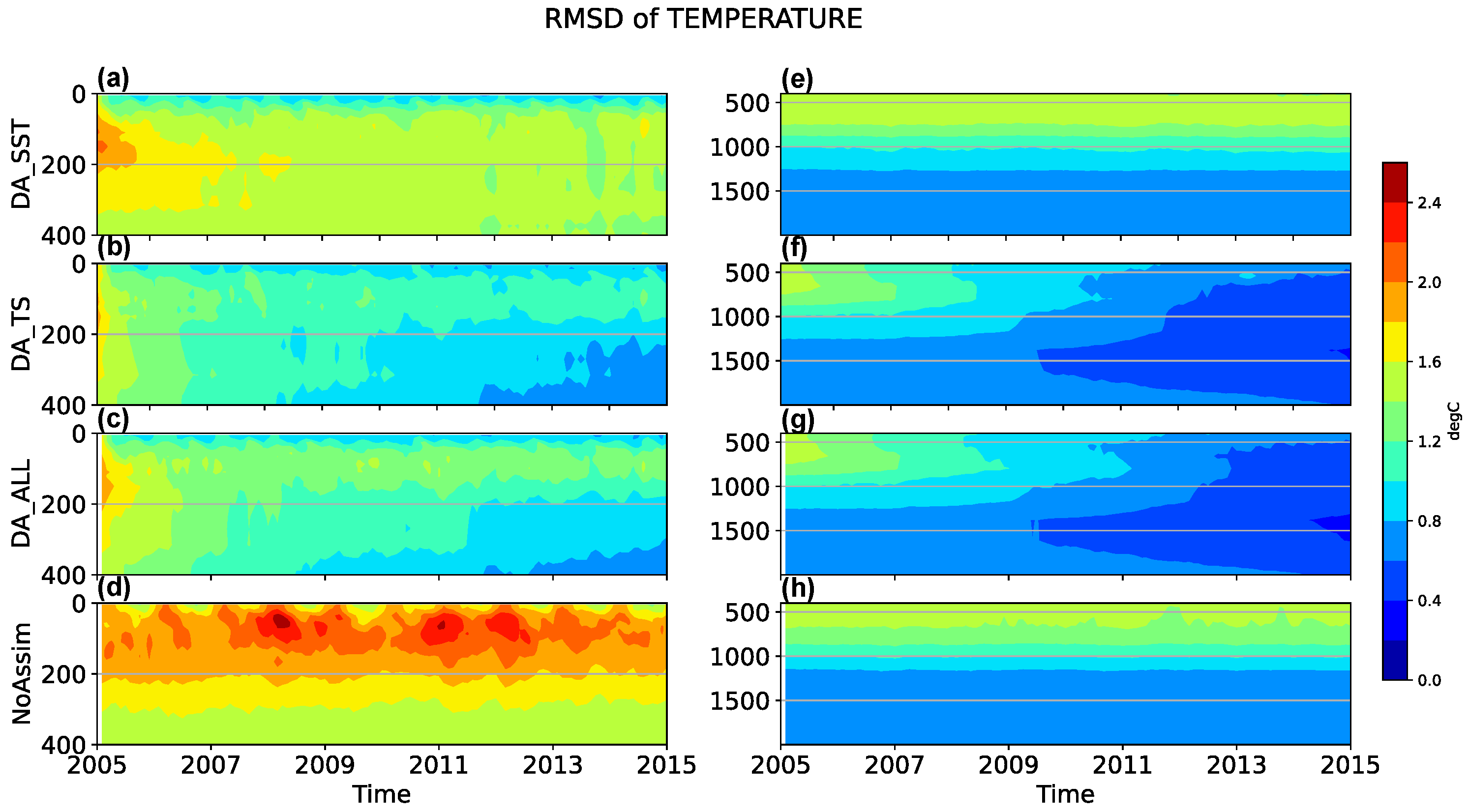
The root mean squared difference (RMSD) relative to the EN4-analysis is employed to assess the performance of data assimilation (DA) methods across various variables and scenarios. Given the substantial errors in the ocean model stemming from biases linked to the sea ice model in higher latitudes, the computation of RMSD is restricted to the range between ${60}^{\circ }$ N and ${60}^{\circ }$ S. Figure 2 illustrates the temperature RMSDs as a function of both depth and time.

The left column displays RMSDs up to 400 m depth, while the right column extends to 2000 m. Comparing DA_SST with NoAssim reveals that SST assimilation primarily influences the upper 300 m, reducing RMSDs in surface and subsurface layers with diminishing returns at greater depths.

In contrast, assimilating TS profiles, as shown in the DA_TS and DA_ALL panels, enhances temperature estimates throughout the water column. Notably, DA_TS achieves lower RMSDs than DA_ALL between 30 and 300 m, suggesting that SST assimilation may counteract the positive effects of TS assimilation. This finding, also observed in EnKF-based DA experiments (e.g., Tang et al. [30] using Local Ensemble Transformed Kalman Filter (LETKF) with AWI-CM), indicates that exclusive TS assimilation yields slightly better temperature estimates.

Although both EnKF and LPF exhibit adverse effects when assimilating SST alongside TS profiles, the underlying mechanisms differ. With EnKF, the Kalman filter updates subsurface temperatures based on correlations with SST, using a localization factor (Equation (A6)) to mitigate spurious correlations among ensemble members. Conversely, LPF determines particle weights from SST (Equation (A7)), which guide the resampling process (Equation (A9)). Here, localization primarily tempers the resampling strength. Thus, assimilating SST after TS may introduce adverse effects through erroneous weights or spurious correlations.

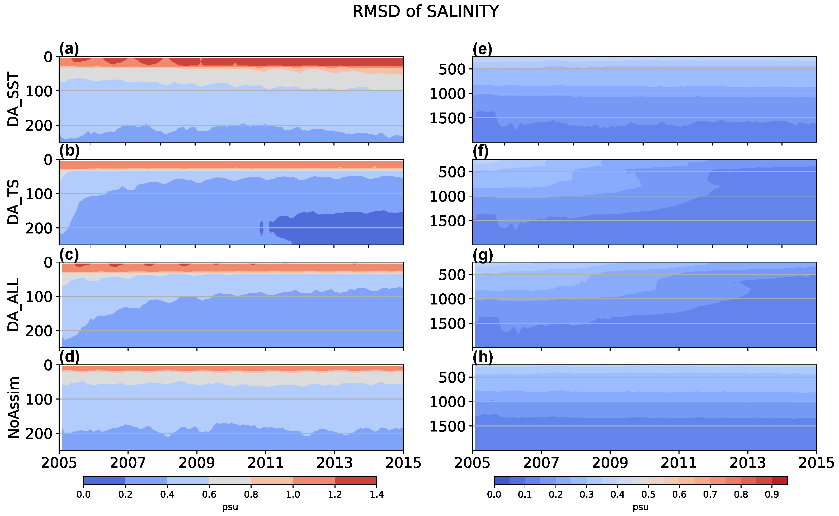
Figure 3 illustrates the salinity RMSDs as functions of depth and time, derived from three DA scenarios and the NoAssim result. Contrary to the results for temperature, assimilating SST exerts a detrimental impact on salinity without yielding any enhancements. It is evident that DA_SST yields analyses with even greater errors than those produced by NoAssim, notably within the upper 300 m of the water column. Additionally, the outcomes from DA_ALL are inferior to those from DA_TS in this region. This strongly suggests that employing weights derived from SST for resampling in salinity is not a sound strategy. Nevertheless, the assimilation of salinity profiles can enhance the simulation of model salinity, particularly at depths less than 1500 m, where salinity observations are adequately available.

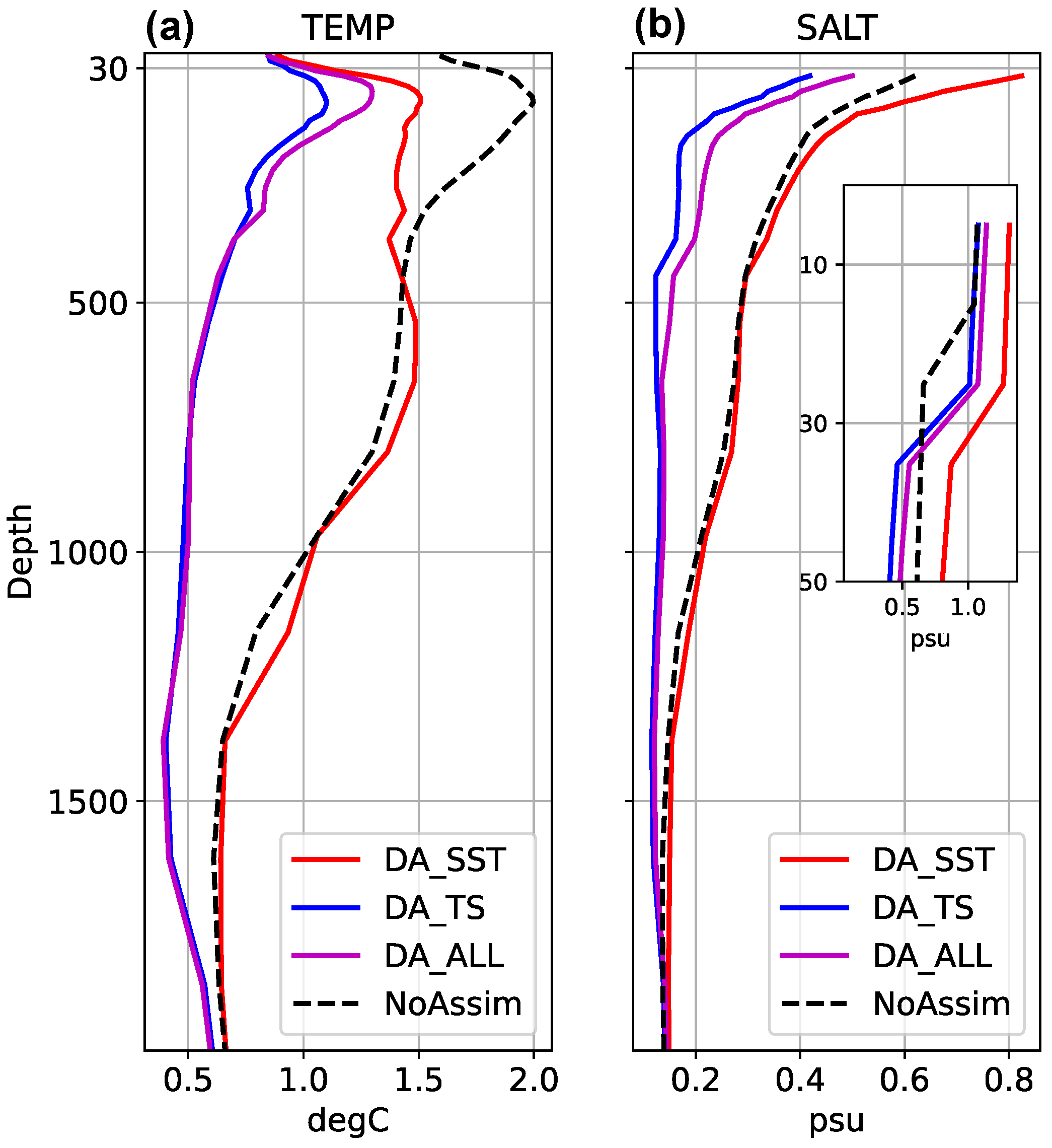
Figure 4 illustrates the temporal average of the RMSD for the year 2014, wherein the RMSD of the assimilation result has attained a saturation level as demonstrated by Figure 2 and Figure 3. The findings further corroborate that while the assimilation of SST enhances temperature accuracy at depths of less than approximately 300 m, it adversely affects salinity compared to scenarios without assimilation (NoAssim). Conversely, the assimilation of TS profiles significantly improves the accuracy of both temperature and salinity measurements at greater depths. Nonetheless, the simultaneous assimilation of SST and TS profiles diminishes the extent of improvement in the precision of temperature and salinity at both surface and subsurface levels.

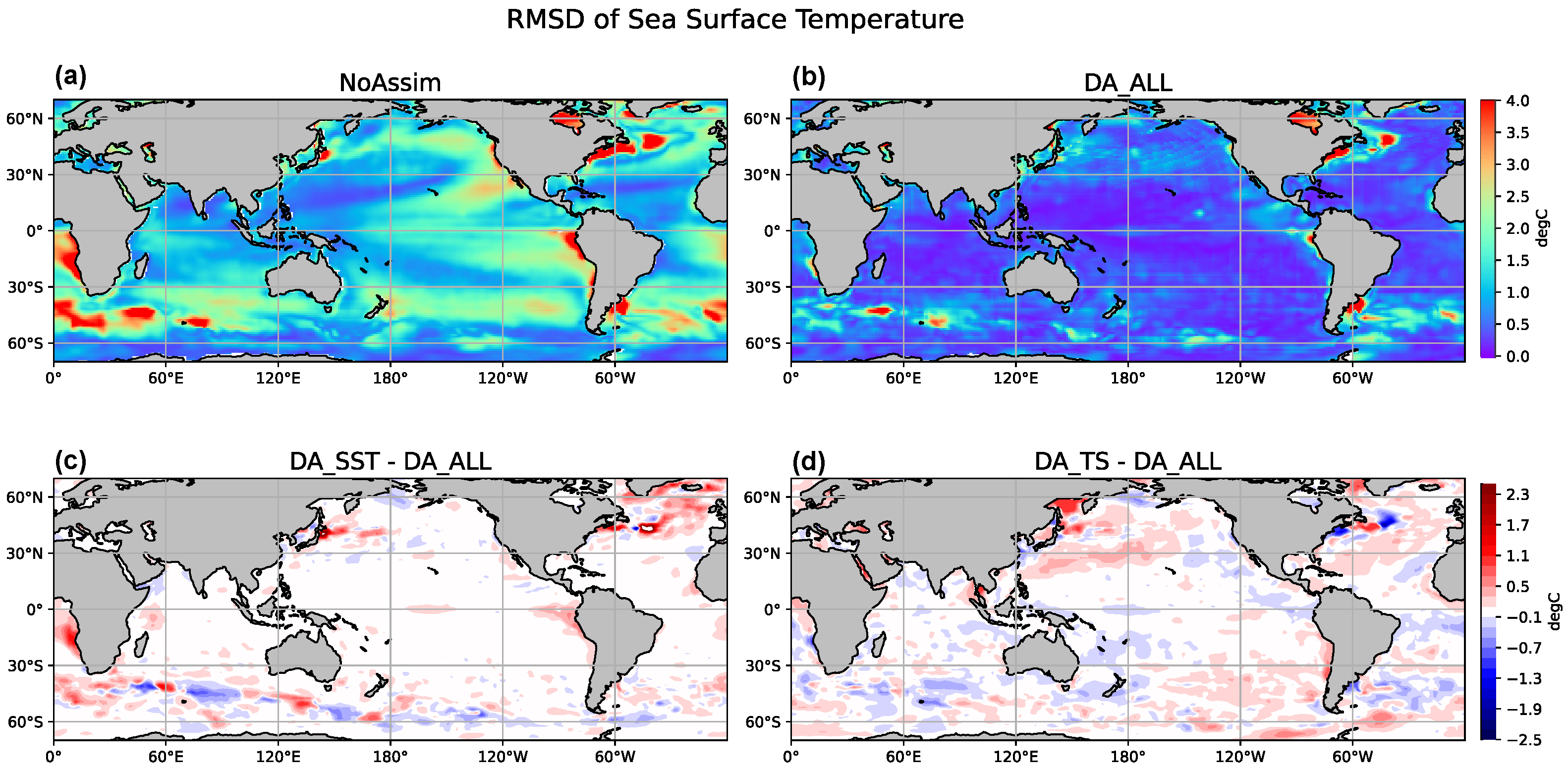
The temporal RMSD of the analysis data, computed over the past year, was utilized to illustrate the spatial distribution of errors. Figure 5b illustrates the spatial distribution of RMSD for SST following the assimilation of all available observations. It is observable that the assimilation of data results in a substantial reduction in SST errors compared to the NoAssim result depicted in Figure 5a. Figure 5c presents the RMSD differences between the outcomes of DA_SST and DA_ALL, highlighting the extent of improvement in the accuracy of the SST variable attributable to the assimilation of TS profiles. In a similar manner, Figure 5d displays the RMSD difference between DA_TS and DA_ALL, illustrating the enhancement in the SST variable’s accuracy owing to the integration of SST observations. Given that gridded satellite SST data offer comprehensive sea surface information, the assimilated SST observations significantly enhance SST accuracy. As demonstrated in Figure 5d, this approach can diminish SST errors across most regions. Conversely, Figure 5c suggests that the assimilation of TS data enhances SST accuracy specifically in the Kuroshio Extension, the North Atlantic Ocean region above ${40}^{\circ }$ N, and the Southern Ocean.

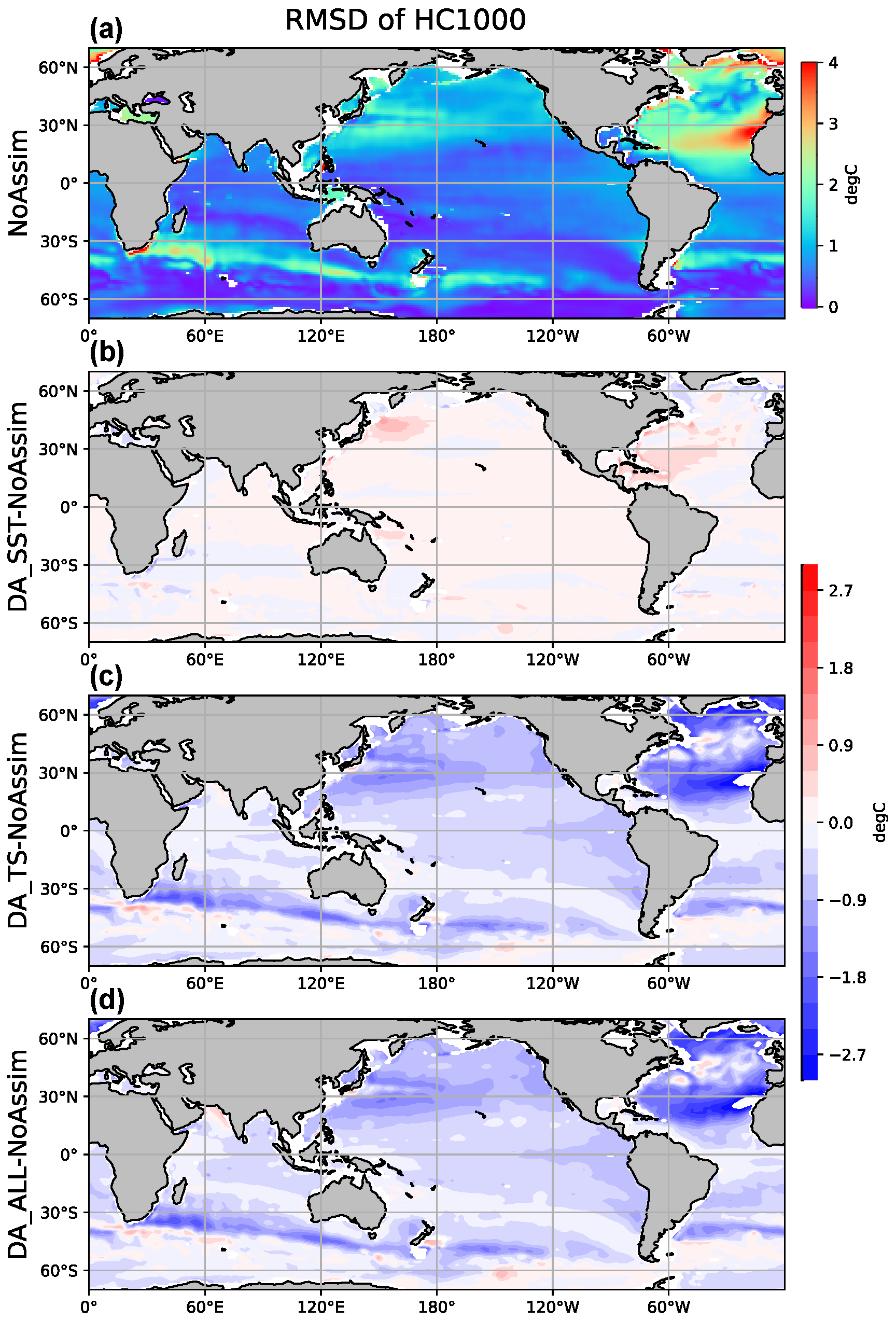
To elucidate the differences between these scenarios at greater depths, we assess the heat content by averaging the temperature field from 500 to 1500 m, which we designate as HC1000. Figure 6 presents the spatial distribution of the temporal RMSD of HC1000 for each experiment throughout 2014. In Figure 6a, considerable errors are identified in the North Atlantic Ocean between ${20}^{\circ }$ N and ${30}^{\circ }$ N in the NoAssim result. As noted by Danabasoglu et al. [20], the deep Atlantic Ocean simulated by CESM tends to be warmer than observed, particularly between ${20}^{\circ }$ N and ${30}^{\circ }$ N at a depth of approximately 1000 m, which is linked to the Mediterranean outflow through the Strait of Gibraltar that is both warmer and saltier than observed. Figure 6b delineates the subtraction of the HC1000 RMSD of the NoAssim result from that of the DA_SST result, affirming the conclusion from Figure 2b and Figure 4a that the assimilation of SST cannot enhance the simulation of deep ocean temperatures, and its influence on HC1000 is adverse. Furthermore, Figure 6c,d exhibit nearly identical RMSD differences derived from DA_TS and DA_ALL outcomes, respectively. This indicates that, on one hand, the assimilation of TS can augment the accuracy of HC1000, while on the other hand, the adverse impact of SST on HC1000 does not extend below 500 m.

4. Comparing with EAKF

To further elucidate the advantages and disadvantages of LPF, we conduct a comparison of the aforementioned DA results with those obtained using the EAKF approach. Chen et al. [18] employed the EAKF method within the DART framework to assimilate SST and TS observations, utilizing the same initial ensembles to assimilate identical observations over the same time period. The DA experiment employing EAKF (referred to hereinafter as DA_EAKF) assimilated SST and TS concurrently, serving as a benchmark for comparison with the results of the DA_ALL experiment utilizing LPF (referred to as DA_LPF). Furthermore, given that DA_TS has demonstrated more accurate analyses compared to DA_ALL, we also incorporate that (referred to hereinafter as DA_LPF(TS)) into the comparison.

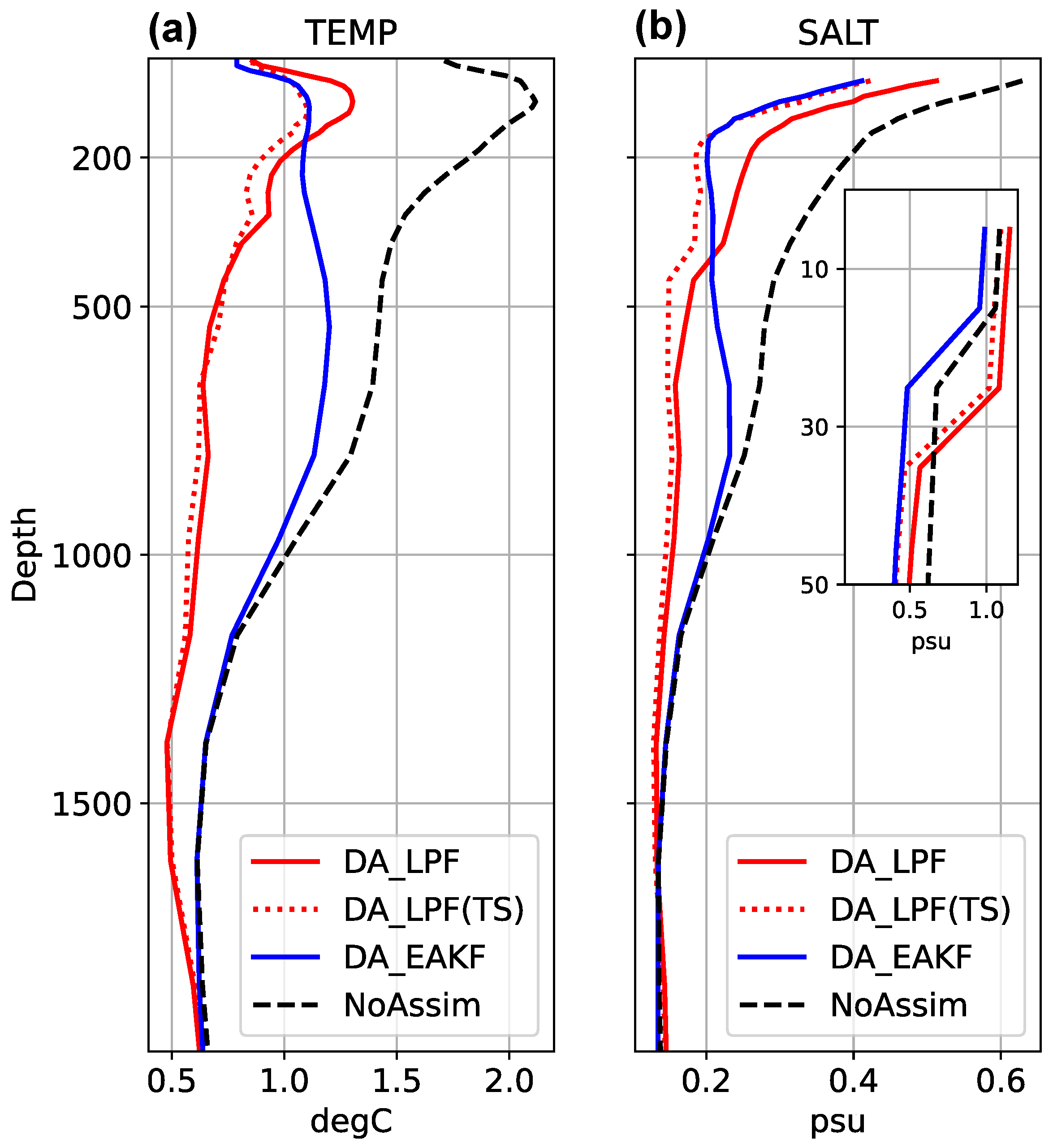
In analogy to Figure 4, Figure 7 illustrates the temporal mean of the RMSD for the year 2014, allowing for the comparison of results derived from DA_LPF, DA_LPF(TS), DA_EAKF, and NoAssim. Figure 7a delineates the RMSD discrepancies concerning temperature. For depths less than 200 m, the EAKF demonstrates superior performance over LPF in enhancing temperature precision. Conversely, DA_LPF(TS) and DA_EAKF show equivalent performance in data assimilation, indicating that SST assimilation via LPF adversely affects its efficacy. Conversely, at depths exceeding 200 m, LPF exhibits a more substantial advancement in temperature analysis. This improvement is plausibly attributed to the capability of LPF to harness the relatively sparse deep observations more effectively.

Figure 7b demonstrates the RMSD discrepancies for salinity. Within the surface layer (depths less than 30 m), the LPF exhibits a detrimental impact on salinity variables, presenting an RMSD that surpasses that of the NoAssim results, in alignment with the discussion in the preceding section. Conversely, the implementation of EAKF enhances the quality of the analysis within the surface layer. Between 30 and 400 m, despite the fact that LPF exerts a positive influence on salinity, its RMSD remains higher compared to EAKF. Nevertheless, when exclusively TS profiles are assimilated, the disparity in performance between LPF and EAKF becomes negligible in the 30–200 m depth interval. This suggests that the assimilation of SST using EAKF positively influences salinity, whereas SST assimilation using LPF exerts a negative influence. Nonetheless, at depths exceeding 400 m, LPF markedly surpasses EAKF.

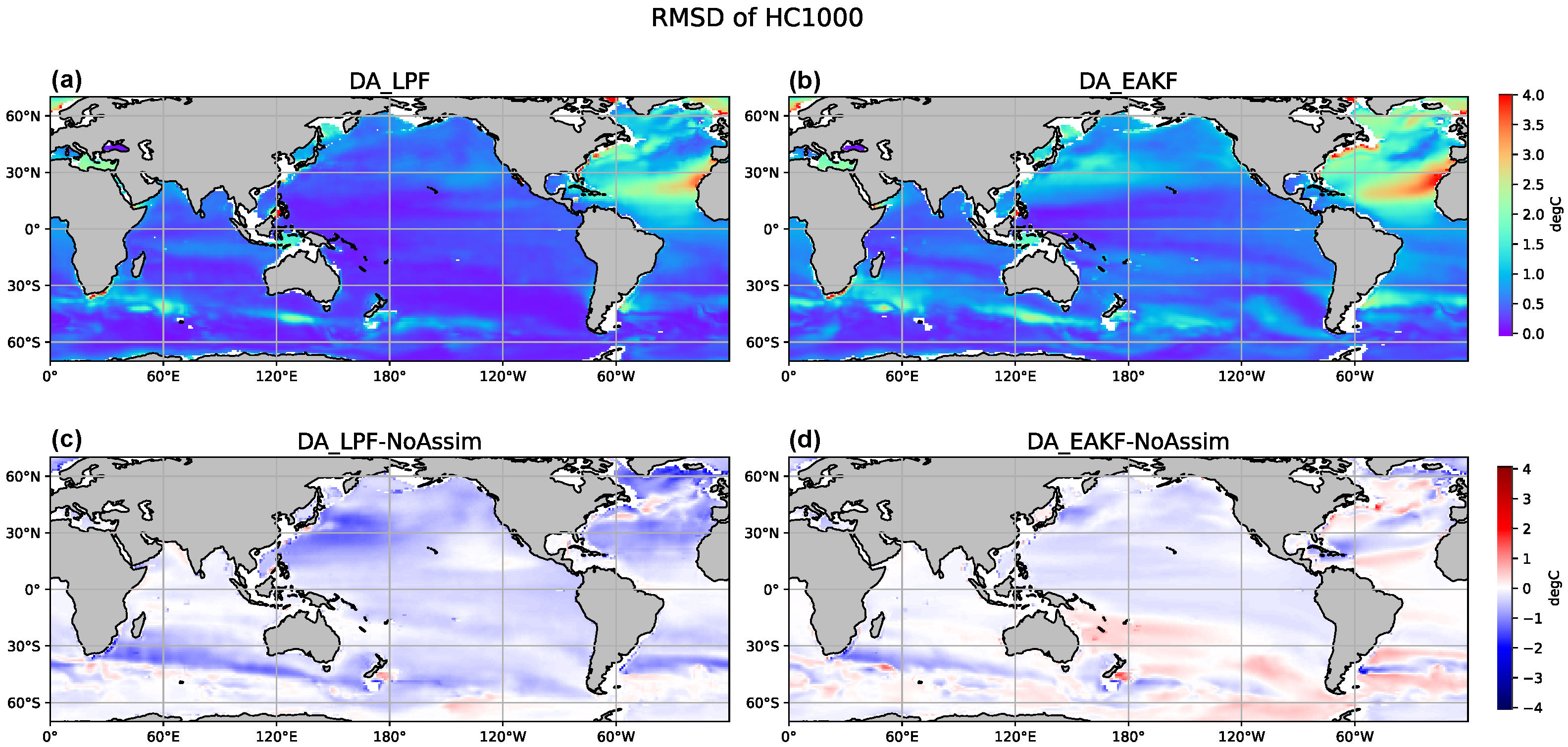
Figure 8a,b depict the RMSD of HC1000 obtained from DA_LPF and DA_EAKF, respectively. Conversely, Figure 8c,d illustrate the difference in RMSD between NoAssim and DA_LPF(DA_EAKF), thereby revealing the extent to which the data assimilation methods mitigate errors. The findings from DA_LPF indicate a significantly reduced RMSD of HC1000 across various regions, with the North Atlantic, particularly between ${20}^{\circ }$ N and ${30}^{\circ }$ N, being notably prominent. As detailed in Figure 6, the NoAssim results display substantial inaccuracies within the deep Atlantic Ocean at an estimated depth of 1000 m, due to the biased Mediterranean outflow through the Strait of Gibraltar. The EAKF method accomplishes only minimal reductions in HC1000 errors within this region as evidenced by Figure 8d. In contrast, the LPF method demonstrates an enhanced capacity to assimilate TS profiles in the deep ocean, substantially decreasing the RMSD of HC1000 in the North Atlantic. Moreover, concerning HC1000, it is apparent that the LPF method outperforms EAKF across the majority of the oceanic domain.

5. Conclusions

In the present study, we have employed the recently developed LPF for the assimilation of CESM, a prevalently utilized CGCM, incorporating actual observational data. The outcomes of the data assimilation are evaluated against the objective analysis data, thereby confirming the potential applicability of the LPF in operational settings. Furthermore, a comparative analysis with the extensively adopted ensemble Kalman filter elucidates the merits and limitations of the LPF, which may facilitate its ongoing development and application.

The comparison results show that LPF could produce a very accurate ocean analysis by assimilating temperature and salinity profiles. However, if LPF is used to assimilate the satellite SST data, it can bring some improvement to the surface and near-surface temperature. But it cannot improve the subsurface and deep ocean temperatures and harms salinity assimilation. Also, the assimilation of SST using LPF in the presence of TS assimilation cannot positively affect the temperature and salinity variables. Since LPF uses weights to perform resampling, it is not as effective as the EnKF for cross-variate updates, which uses linear regression to update different model variables according to the correlation.

The adverse impact of additionally assimilating SST can be traced to the intrinsic limitations of the LPF mechanism. Once TS profiles have supplied depth-dependent particle weights, the subsequent introduction of SST triggers a second, competing weight adjustment. Because LPF relies on localized Monte Carlo resampling rather than the EAKF linear regression, its influence decays sharply with distance from the surface; the new weights therefore distort the already adequate deep-ocean weights without providing compensating information. The result is an over-shrinkage of spread near the surface and spurious increments at depth, degrading both temperature and salinity estimates. This illustrates that, for LPF, the mere availability of extra observations does not guarantee benefit; the judicious selection and sequencing of data streams is essential.

Therefore, when solely temperature and salinity profiles are assimilated, the LPF methodology exhibits a pronounced superiority over EAKF, particularly concerning the representation of temperature and salinity within the subsurface and deep ocean strata. Notably, LPF is adept at mitigating substantial discrepancies in the deep Atlantic Ocean, approximately at a depth of 1000 m, attributable to the biased Mediterranean outflow via the Strait of Gibraltar, which may hold potential benefits for enhancing the simulation of the Atlantic Meridional Overturning Current (AMOC). The underlying causes for the superior performance of LPF in the subsurface and deep ocean primarily encompass two aspects: firstly, the small variability of deep-ocean temperature and salinity yields correspondingly small entries in the background–error covariance matrix, which under an insufficient ensemble size degrades the effectiveness of the EAKF linear-regression update; secondly, the intrinsic nonlinear and non-Gaussian characteristics of LPF may facilitate the assimilation of deep variables that are commonly underobserved.

In conclusion, LPF can be used for the practical assimilation of complicated CGCMs and has great potential for enhancing the assimilation processes in certain non-Gaussian and nonlinear systems. Nonetheless, this study focuses solely on the assimilation results of temperature and salinity, without yet integrating the assimilation of sea surface height (SSH). Furthermore, despite employing a fully coupled earth system model for the experiments, the assimilation is limited to ocean observations within a weakly coupled data assimilation (DA) framework. Although the LPF may ultimately prove even more valuable within a strongly coupled framework, such configurations remain an open challenge: even state-of-the-art EnKF- or 4D-Var-based strongly coupled data assimilation implementations have yet to provide definitive solutions because capturing cross-component covariances demands ensemble sizes far larger than those required for the cross-variable updates examined here. The present study therefore focuses on demonstrating LPF viability under weakly coupled conditions and benchmarking it against prior EAKF experiments conducted within the same framework; extending the LPF to strongly coupled data assimilation will be pursued in future work.