Abstract
Temporal variability in emissions from oil and gas supply chains depends on the spatial scale at which emissions are aggregated. This work demonstrates a framework for simulating temporally and spatially resolved emission inventories that can be broadly applied in oil and gas production regions. Emissions of methane, ethane, volatile organic compounds (VOCs), and nitrogen oxides (NOxs) from oil and gas facilities in the Marcellus production region were estimated at a one-hour time resolution for the calendar year 2023 and were aggregated at the grid cell (4 km by 4 km), county, and basin level. Maximum to average emission rate ratios decreased as the scale of spatial aggregation increased and differed by pollutant. At the grid cell level, ratios of maximum to average emission rates exceeded 100 in some grid cells for VOCs. In contrast, basin level maximum to average ratios for NOx emission rates were less than 1.1. The sources driving temporal variability in hydrocarbon emissions were well completions and liquid unloadings, while the sources driving temporal variability in NOx emissions were preproduction activities such as drilling and hydraulic fracturing. Temporally and spatially resolved inventories can inform pollutant- and region-specific measurement campaigns and mitigation strategies. Reconciliation between inventories and observations must consider event frequency, duration, and persistence, along with the spatial scale and timing of measurements.
1. Introduction
Emissions of greenhouse gases and criteria air pollutants from oil and gas supply chains have complex spatial and temporal patterns [1]. For example, emission rates for methane from individual sources can vary over six orders of magnitude, from grams per hour to tons per hour [2], but the highest emission rate sources generally have short durations, while lower emission rate sources can be both long and short duration [3]. If ensembles of instantaneous measurements are made at oil and gas production sites, methane emissions follow a highly skewed distribution, with the sites with the highest instantaneous emission rates (top 5%) contributing >50% of total emissions [4]. The overall magnitude of emissions and their spatial and temporal patterns can vary by basin. Collectively, and integrated over time, production-normalized methane emissions at the basin level ranged from <1% to 5% among major oil and gas basins in the United States [4,5]. Emissions of volatile organic compounds (VOCs) also have temporal and spatial variability [6], but the sources of that variability are different than the sources of variability in methane and other light alkane emissions [7]. Emissions of nitrogen oxides (NOxs) also exhibit variability [8], but again, the sources are different than the sources that drive variability in methane and VOCs emissions [9].
The magnitude of temporal variability in emissions depends not only on the pollutant but also on the spatial scale at which emissions are aggregated. The smaller the spatial scale of aggregation, the larger the temporal variability. Discrete measurement campaigns at the same well site showed significant variability in methane emissions, with emission rates varying by nearly 50-fold across six measurement campaigns over a 21-month period [10] and by more than 550 times across 17 campaigns conducted over four years [11]. Even greater variability will be observed if emissions are monitored continuously [12,13]. Temporal variability in emissions from individual sites will generally be greater than variability in emissions aggregated over a grid cell containing dozens of sites; grid cell variability will be greater than the variability at the county level, which will be greater than the variability at the basin level. No prior research has systematically examined how temporal variability in emissions vary, as emissions are aggregated across various spatial scales.
There are multiple human health implications associated with spatial and temporal variability in emissions. Examples of potential impacts include, but are not limited to, variability in ozone productivity driven by local variability in emissions of NOx, particularly when coupled with high emissions of biogenic hydrocarbons and localized exposures to elevated levels of criteria or hazardous air pollutants [9]. Spatial and temporal variability in emissions is also important to consider when using short duration measurements, such as aircraft overflights, in estimating longer term emissions. The magnitude, frequency, and duration of episodic emissions will determine how many measurements will be needed to accurately predict long-term emissions [14,15,16].
This work will demonstrate methods for modeling spatial and temporal variability in emissions from oil and gas sources by estimating the routine emissions associated with the production and midstream processing of oil and gas produced by more than 200,000 sites in the Marcellus production region in the United States. Year-long time series of emissions will be estimated at one-hour resolution for methane, ethane, VOCs, and NOx. Emissions will be aggregated at the grid cell (4 km by 4 km), county, and basin level, and at each of these spatial scales, distributions of expected emission rates will be characterized.
The framework and simulation methods developed in this work can be broadly applied in other oil and gas production regions to characterize both spatial and temporal variability in hydrocarbon and NOx emissions. Understanding these pollutant-specific temporal and spatial characteristics is essential for developing pollutant-specific measurement campaigns and mitigation strategies. Current national and regional emission inventories, such as the U.S. Greenhouse Gas Inventory (GHGI) [17], the National Emissions Inventory (NEI) [18], the Greenhouse Gas Reporting Program (GHGRP) [19], and emission inventories developed by state governments for air quality management [20], typically report annual average emissions and do not capture temporal variability in emissions from oil and gas sources. This work provides a pathway to develop spatially and temporally resolved emission inventories based on publicly available information and enables a more accurate representation of emissions. Inventories for the Marcellus oil and gas production region in the northeastern United States are developed to demonstrate the methods.
2. Materials and Methods
2.1. Study Domain
Figure 1 shows the study domain and locations of simulated sources. The study domain was divided into 4 km by 4 km grid cells covering 98% of active production wells reported in the Marcellus Shale [21]. A total of 201,338 wells, drilled on or before 2023 and actively producing in 2023, are included in the simulation, representing production and emission scenarios in the year 2023. The gridded area includes grid cells without any reported production, and these grid cells will be assumed to have no emissions associated with upstream and midstream oil and gas operations.
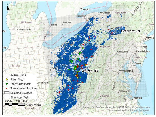
Figure 1.
Well sites, midstream sites, and flares included in the simulation within the study domain overlapped by 4 km-by-4 km grid cells.
Emission sources in the study domain include well-level emissions from preproduction and production activities on active well sites, emissions from midstream operations, and emissions from flaring. Active well sites were identified based on production data [21]. Well site emissions in two counties, Bradford, PA, USA and Wetzel, WV, USA were used as representative regions to compare county-level emissions to emissions resolved at the grid cell level. Bradford County is located in the northeast portion of the basin, a relatively dry gas production region with mostly unconventional horizontally drilled wells. Wetzel County is in the southwest portion of the basin and has a large amount of liquids production compared to Wetzel County, from comparable numbers of conventional and unconventional wells. Distributions of well types included in the study domain and in two selected counties are shown in Table 1. Aggregated production data in the study domain and in the two selected counties are available in Supporting Information (SI).

Table 1.
Well types in the study domain and two selected counties.
Midstream sites include gathering and boosting stations (assumed one per grid cell), gas processing plants, and transmission facilities. Gas processing plants and transmission facilities were drawn from the EPA Greenhouse Gas Reporting Program (GHGRP) [19] and manually verified based on satellite images [22]. Flare locations were based on annual gas flare estimates with Visible Infrared Imaging Radiometer Suite (VIIRS) observations in 2023 [23]. Only midstream flares and flares located in grid cells with active wells were included in the simulation.
2.2. Spatial Aggregation
Emissions were aggregated and are reported at three spatial levels: the grid cell level, the county level, and the basin level. These levels of reporting involved 2 types of aggregation: pre-simulation and post-simulation. Pre-simulation refers to the aggregation of activity data (e.g., production volumes and equipment counts) prior to emission simulation. Post-simulation refers to the aggregation of simulated emissions. Post-simulation aggregation at individual well sites and midstream sites was carried out in Bradford and Wetzel Counties. These simulations will be used to compare grid-cell-level aggregation of emissions to county-level aggregation of emissions. To compare county-level aggregation of emissions to basin-level aggregation of emissions, sources were aggregated pre-simulation at the county level.
For wells in Bradford and Wetzel Counties, well site emissions were simulated based on estimated equipment and operation counts at individual well sites. Emissions from gathering, processing, and transmission sites and flares were simulated as total site-level emissions. These emissions were spatially aggregated by grid cell and by county over the 2023 year-long time series. Bradford County includes a total of 1520 wells, with 1216 wells located within 132 grid cells that are completely within the county boundary. Wetzel County includes 1295 wells, with 840 wells distributed across 36 grid cells that are fully within the county. Only wells within grid cells that are completely within county boundaries were included in spatial aggregation.
For county-level and basin-level reporting based on county-level simulations, well sites were aggregated pre-simulation. Up to three “aggregated wells” were created for each county: one dry gas well representing all dry gas wells, one wet gas well representing all wet gas wells, and one oil well representing all oil wells within the county. Production volumes and equipment counts were summed and assigned to their corresponding aggregated well. Detailed aggregation and simulation methods, by source, are described in the following sections.
2.3. Emission Compositions
Emission compositions at the well level were simulated using the Emission Composition Tool, built into the Methane Emission Estimation Tool (MEET V1.1) [24]. The Emission Composition Tool is a searchable database constructed with field measurement data and thermodynamic models and can be queried to estimate hydrocarbon compositions from various emission sources at oil and gas production sites by matching input parameters, including gas-to-oil ratios, API gravity, separator temperature and pressure, and produced gas compositions [25]. Three emission composition profiles were generated in this work: dry, wet, and oil. Input parameters for “dry” and “wet” profiles were estimated based on the averaged parameters from dry gas and wet gas wells measured in the Marcellus production region [26]. Input parameters for the “oil” profile were from multiple sources. Gas-to-oil ratio was calculated based on production data in the basin in 2023 [21]. API gravity, separator pressure, and produced gas compositions were the averaged values across a subset of wells from the Central Appalachian Basin Natural Gas Database [27]. The subset included wells with an API gravity lower than 45 and non-zero produced gas compositions. While the database did not provide information on separator temperature, separator temperature for the “oil” profile was assumed to be the same as that for the “wet” profile. Input parameters for estimating each composition profile are summarized in Table 2.
Table 2.
Input parameters for estimating emission compositions using the Emission Composition Tool.
Table 3 shows estimated emission compositions returned by the Emission Composition Tool [25], based on input parameters in Table 2. Four sets of emission compositions were estimated for each composition profile, including wellstream, produced gas, water tank flash, and condensate tank flash. While the tool did not simulate VOC emissions from condensate tank flash, the sum of propane and butane emissions was used as a surrogate for VOCs and is reported in Table 3. Emission compositions from the dry composition profile were assigned to emissions from dry gas wells; wet profile compositions were assigned to wet gas wells, and oil profile compositions were assigned to oil wells. There were a few wells characterized as dry gas wells in the production database [21] but with non-zero oil production. Since the dry profile assumed no oil production, wet profile compositions were re-assigned to these wells.
Table 3.
Estimated emission compositions applied in inventory development.
2.4. Emission Sources
Table 4 summarizes all emission sources and pollutants included in the simulation, the emission estimation method and hydrocarbon compositions for emission estimates, and whether the source was aggregated pre-simulation for county- and basin-level reporting. Hydrocarbon compositions were sourced from the EPA 2020 Nonpoint Oil and Gas Emission Estimation Tool (referred to as EPA Oil and Gas Tool in the following text) [28], and/or from the Emission Composition Tool [25]. The 2020 version of the EPA Oil and Gas Tool was used because it was the most recent version with complete documentation at the time the simulations were performed. The composition of throughput gas for midstream facilities and the composition of flared gas at the grid cell level was estimated by combining production and produced gas compositions from individual wells. Throughput gas compositions estimated at the level of counties were used to estimate emissions from combustion sources that included artificial lift engines and heaters, assuming local produced gas was used as fuel. The sources without pre-simulation aggregation were always simulated at the individual well level and aggregated during post-processing.
For some of the simulated sources, activity data used in equipment assignments were sourced from the 2022 Inventory of U.S. Greenhouse Gas Emissions and Sinks (GHGI) [29], shown in Table 5. The 2022 data was the most recent version available at the time the simulations were performed. The GHGI reports two sets of activity factors for the natural gas system and the petroleum system. Activity factors reported for the natural gas system were applied to dry gas wells, and activity factors reported for the petroleum system were applied to the oil wells. For wet gas wells, the activity data was assigned as the average data for dry gas and oil wells. If the equipment or operation category does not exist in the petroleum system, or is not applicable to oil wells, such as gas meters/piping and liquid unloading operations, the activity factors reported for the natural gas system were consistently applied to both dry and wet gas wells. The equipment assignments based on this activity data are described in the Supporting Information (SI).
Detailed simulation methods per emission source are available in the SI. Briefly, emissions per source were simulated by combining activity factors, emission factors, and composition data from various publicly available databases. Hydrocarbon emissions from most non-combustion sources at well sites were simulated using the Methane Emission Estimation Tool (MEET) V1.1 [24]. Hydrocarbon emissions from associated gas venting and hydrocarbon and NOx emissions from combustion sources at well sites were simulated using the EPA Oil and Gas Tool [28]. Hydrocarbon emissions from gathering and boosting sites were estimated based on throughput gas flowrates and compositions. Hydrocarbon emissions from gas procession and transmission sites were estimated based on the EPA Greenhouse Gas Reporting Program [19] and throughput gas compositions. NOx emissions from gathering and boosting, processing, and transmission sites were estimated based on methane emissions, fraction of combustion sources, and the EPA AP-42 emission factors for stationary internal combustion sources [30]. For flares, hydrocarbon emissions were estimated based on satellite detections, and NOx emissions were estimated based on methane emissions and EPA AP-42 emission factors for flaring [30].
The simulation methods for well site non-combustion sources were evaluated against observations by Graves et al. [31]. Simulated ethane inventories coupled with site-level dispersion modeling for thousands of sites were summed and compared with ethane measurements at a regional air quality monitor in the Eagle Ford oil and gas production region. Predictions of routine emissions, coupled with dispersion modeling, accurately captured diurnal profiles of observations up to the 95th percentile of observations. Simulated routine emissions accounted for one third of the highest (>99th percentile) daytime concentrations observed and two thirds of the highest nighttime concentrations observed.
Table 4.
Emission sources and estimation method.
Table 4.
Emission sources and estimation method.
| Emission Sites | Emission Sources | Simulated Pollutants | Main Method for Emission Estimates | Hydrocarbon Compositions | Pre-Aggregation |
|---|---|---|---|---|---|
| Well sites: preproduction | Drilling engines | Methane, VOCs, NOx | EPA Oil and Gas Tool [28] | EPA Oil and Gas Tool | Not aggregated |
| Hydraulic fracturing pumps | Methane, VOCs, NOx | EPA Oil and Gas Tool [28] | EPA Oil and Gas Tool | Not aggregated | |
| Completion flowbacks | Methane, Ethane, VOCs | MEET [24] | Wellstream | Not aggregated | |
| Well sites: production | Artificial lift engines | Methane, ethane, VOCs, NOx | EPA Oil and Gas Tool [28] | County-throughput-produced gas composition and EPA Oil and Gas Tool | Aggregated |
| Associated gas venting | Methane, ethane, VOCs | EPA Oil and Gas Tool [28] | Produced gas | Aggregated | |
| Condensate tank flash | Methane, ethane, VOCs | MEET [24] | Condensate tank flash | Aggregated | |
| Water tank flash | Methane, ethane, VOCs | MEET [24] | Water tank flash | Aggregated | |
| Leaks | Methane, ethane, VOCs | MEET [24] | Varying compositions | Aggregated | |
| Pneumatic controllers | Methane, ethane, VOCs | MEET [24] | Produced gas | Aggregated | |
| Chemical injection pumps | Methane, ethane, VOCs | MEET [24] | Produced gas | Aggregated | |
| Heaters | Methane, ethane, VOCs, NOx | EPA Oil and Gas Tool [28] | County-throughput-produced gas composition and EPA Oil and Gas Tool | Aggregated | |
| Liquid unloadings | Methane, ethane, VOCs | MEET [24] | Produced gas | Not aggregated | |
| Gathering and boosting | Total site emissions | Methane, ethane, VOCs, NOx | Zimmerle et al. [32] | Grid-cell-throughput-produced gas | Not applicable |
| Gas processing sites | Total site emissions | Methane, ethane, VOCs, NOx | GHGRP [19] | Grid-cell-throughput-produced gas | Not applicable |
| Gas transmission sites | Total site emissions | Methane, ethane, VOCs, NOx | GHGRP [19] | Grid-cell-throughput-produced gas | Not applicable |
| Flare | Flare emissions | Methane, ethane, VOCs, NOx | VIIRS [23] | Grid-cell-throughput-produced gas | Not applicable |
Table 5.
Activity data extracted and calculated from EPA GHGI for selected sources.
Table 5.
Activity data extracted and calculated from EPA GHGI for selected sources.
| Simulated Source | Equipment | Unit | Dry Wells | Wet Wells | Oil Wells |
|---|---|---|---|---|---|
| Leaks | Meter/piping | Count per well | 0.93 | NA | |
| Chemical injection pumps | Chemical injection pumps | Count per well | 0.03 | 0.01 | 0 |
| Pneumatic controllers | Pneumatic controllers | Count per well | 0.97 | 0.63 | 0.29 |
| High bleed | Fraction | 0.2% | 0.1% | 0% | |
| Low bleed | Fraction | 17.3% | 23.4% | 43.8% | |
| Intermittent bleed | Fraction | 82.5% | 76.6% | 56.7% | |
| Heaters | Heaters | Count per well | 0.1 | 0.06 | 0.02 |
| Liquid unloading | Unloadings with plunger lifts | Fraction | 4.0% | NA | |
| Unloadings without plunger lifts | Fraction | 6.8% | NA | ||
3. Results
Hourly emissions time series for methane, ethane, VOCs, and NOx are presented—aggregated at the grid cell, county, and basin level—in Figure 2, Figure 3 and Figure 4. In Figure 2, Figure 3 and Figure 4, emissions from well site preproduction activities, including drilling engines, hydraulic fracturing pumps, and completion flowbacks, were aggregated as the source category “completion/drilling/fracturing”; emissions from well site pneumatic controllers and chemical injection pumps were aggregated as the source category “pneumatic devices”; emissions from condensate tank flash and water tank flash at well sites were aggregated as “tank flash”; emissions from artificial lift engines, associated gas venting, heaters, and leaks on well sites were aggregated as “wellsite—other routine emissions”; emissions from gathering and boosting sites, gas processing sites, and transmission sites were aggregated as “gathering/processing/transmission”; emissions from flares and emissions from liquid unloadings on well sites were presented individually. Time series of emissions by individual source are available in the SI. Time series for additional grid cells and an additional county are presented in Supporting Information (SI). The selected grid cell presented in Figure 2 is located in Wetzel County, WV. It contained 70 actively producing wells in 2023, 11 of which were completed in 2023. Six wells were assigned liquid unloadings. Detailed well characteristics of selected grid cells are available in the SI.
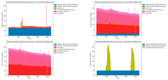
Figure 2.
Hourly emissions time series for methane, ethane, VOC, and NOx emissions in a selected grid cell in Wetzel, WV.
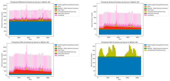
Figure 3.
Hourly emissions time series for methane, ethane, VOC, and NOx emissions in Wetzel County, WV.
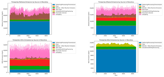
Figure 4.
Hourly emissions time series for methane, ethane, VOC, and NOx emissions in the basin.
At the grid cell and the county level, though episodic emission sources such as liquid unloadings and preproduction activities dominate temporal variations in hydrocarbon emissions, total hydrocarbon emission rates generally decline as total production rates decline, and increase when total production rates increase, due to high initial production rates of the new wells completed. Such temporal declines were mainly driven by emissions from tank flash and are consistent with the projected temporal evolution of methane emissions from oil and gas production sites [33]. Compared to methane emissions, ethane and VOC emissions showed a larger relative decline because tank flash emissions contribute to a higher fraction of ethane and VOCs’ totals. However, at the basin level, such temporal declines were not observed because of the relatively stable production aggregated at the basin level.
In Wetzel County, WV, methane emissions were primarily driven by gathering operations, with significant emission spikes from unloading events and occasional high-emission-rate completion events. Ethane and VOC emissions showed similar temporal patterns to those of methane, with greater contributions of emissions from condensate tank flashing. County-level ethane and VOC emissions from condensate tanks declined as existing wells aged and increased when new wells began production. In contrast, county-level methane emissions showed less sensitivity to this production change. Temporal variations in NOx emissions were driven by episodic, clustered drilling and fracturing events. In comparison, in Bradford County, PA, a dry gas production region with a comparable fraction of wells completed in 2023, temporal variability in total regional NOx emissions driven by preproduction activities was smoothed out due to the consistent high emissions from gathering operations. However, VOC emissions in Bradford were more significantly influenced by preproduction activities, in which drier gas was produced and no condensate tanks were present. Time series emissions in Bradford, PA, are available in the SI.
At the grid cell level, temporal variations in hydrocarbon emissions were primarily driven by liquid unloading and well completion events. In the absence of these events, emissions from pneumatic controllers also contributed to grid-level temporal variability (see SI Figures S4-2 and S4-6. NOx emissions were either relatively constant throughout the year or showed temporal variations driven by preproduction operations and flaring (see SI Figure S4-8).
At the basin level, spatial aggregation reduced the impact of intermittent events, especially for NOx emissions. Hydrocarbon emissions retained more temporal variations due to short, frequent, and high-rate events such as liquid unloadings and well completions. Pneumatic controllers, switching between low-emitting normal modes and high-emitting abnormal modes, also contributed to temporal variability at the basin level, particularly for methane and ethane.
Table 6 presents statistics of methane, ethane, VOC, and NOx emissions for the basin, Wetzel County, and the selected grid cell in Wetzel County, WV, as shown in Figure 2. Table 7 and Table 8 summarize ratios of maximum to annual average hourly predicted emission rates and the distribution of calculated ratios at various spatial levels. Additional summary tables for Bradford, PA, are available in the SI. Maximum to average emission rate ratios decreased as the scale of spatial aggregation increased because spatial aggregation masks emissions intermittency. For example, the ratio of maximum to average emission rate for VOC emissions was 1.6 at the basin level and 5.8 in Wetzel County. At the grid cell level, this ratio exceeded 100 in some grid cells within Wetzel County, WV. Compared to hydrocarbon emissions, NOx emissions presented less temporal variability in most counties, since NOx emissions were dominated by continuous emissions from gathering, processing, and transmission sites at most times. Exceptions are in the counties with little current production but with occasional preproduction activities for new wells. In these counties, NOx emissions were dominated by episodic emissions from preproduction activities and showed greater temporal variations. Maximum to average ratio for NOx emission rates was 1.1 and 1.4 at the basin level, and in Wetzel County, WV, respectively. The sources driving temporal variability for hydrocarbon emissions were liquid unloadings and well completions, while the sources driving temporal variability in NOx emissions were preproduction activities such as drilling and hydraulic fracturing. At finer spatial scales such as the grid cell level, NOx emissions from flares can also lead to elevated emission rates (see SI).
Table 6.
Distributions of methane, ethane, VOC, and NOx emission rates for the basin, Wetzel County, and the selected grid cell.
Table 7.
Ratios of maximum to annual average hourly predicted emission rates at the basin and county levels and distributions of the ratios among 173 counties included in the basin.
Table 8.
Ratios of maximum to annual average hourly predicted emission rates at a selected grid cell level and distributions of the ratios among 36 grid cells located within Wetzel County, WV.
4. Discussion
Although this work focuses on the Marcellus basin, the simulation framework and methods developed in this work can be broadly applied in other oil and gas production regions. Temporal variations in emissions may change depending on production characteristics in the region. For example, in the Permian Basin where the majority of wells are oil producing wells, fewer emissions from liquid unloadings occur [34] and less temporal variations are expected. The ability to simulate temporally resolved emissions at various spatial levels is important in basins with varying production characteristics. For example, the Eagle Ford Shale has subregions with distinct production profiles, ranging from oil-dominated regions to wet gas and dry gas production regions [35]. Basin-level estimates cannot accurately represent the emission characteristics in sub-regions within the basin. Dominant emission sources and temporal variations in emissions vary within the basin. The sources that dominate temporal variations in emissions vary by pollutant, and results from this work are consistent with prior published measurements and inventories. For example, a top-down/bottom-up methane emission reconciliation study reported that episodic emissions from manual liquid unloadings drive temporal variations in the basin-level emission rates by a factor of two [14].
Methods for reconciling these predicted time series with measurements will vary depending on the intermittency in emissions predicted and the type of measurement being made. For example, satellite or aircraft measurements could be made to estimate total area-wide emissions at the scale of a county or basin. In these cases, if emissions are relatively constant over the time-scale of a day, such as for NOx, then the average emission estimate for the day could be compared to the instantaneous measurement made by a satellite or an aircraft performing a mass balance flight. There is, however, day-to-day variability in emissions, and in the case study considered in this work, that day-to-day variability at a county level can be 20% or more.
Reconciliations between predicted emission inventory time series and observations are more complex when emissions have durations of less than a day or have a diurnal pattern. This is the case for unloading emissions in the Marcellus region. Consider a county with 1000 wells (similar to Wetzel County), where 10% of the liquid unloadings lead to venting, and each well vents 10 times per year. This would lead to an expected value of 1000 venting events per year. If the venting was distributed evenly throughout the day, then three unloadings would be expected on any day. In contrast, if the unloadings only occur during an 8 h working period, nine unloadings would be expected in each working day, when measurements from aircraft and satellites are typically made. If the unloadings were distributed uniformly throughout the working day, and each lasted slightly less than an hour, then at any given time during the working day, one unloading should be observed in a county. In contrast, if unloadings were distributed uniformly throughout the day, then only on one day in three would an hour-long unloading be observed during an instantaneous measurement in the hypothetical county. If the duration of the events was 30 min instead of an hour, the expected frequency for observing unloadings would be cut in half.
These simple examples illustrate the care that must be taken in comparing predicted intermittent, short duration events with observations. Accurate comparisons will depend on the frequency, duration, and diurnal patterns of the emission events [15]. For large emission rates such as blowdowns or unloadings, a single event at a single site can have a significant impact on the instantaneous emission rates at the scale of a basin or county [14]. Emission predictions, accounting for emission intermittency and diurnal variations, should be compared to observations at the time that measurements are made.
5. Conclusions
Hourly emissions of methane, ethane, VOCs, and NOx were estimated for the calendar year 2023 across more than 200,000 well sites in the Marcellus oil and gas production region. Emissions were aggregated in terms of 4 km-by 4-km grid cells, counties, and the basin. Temporal variability in emissions increased at finer levels of spatial aggregation and varied by pollutant. Hydrocarbon emissions, dominated by episodic events such as liquid unloadings, have larger temporal variations compared to NOx emissions, which are dominated by combustion sources with relatively consistent emission rates. The sources that drive temporal variations in hydrocarbon emissions were liquid unloadings, whereas the sources that drive temporal variations in NOx emissions were drilling and fracturing activities.
The framework presented in this work is broadly applicable in other oil and gas production regions, and the ability to simulate temporally and spatially resolved inventories enables the development of pollutant- and region-specific measurement campaigns and mitigation strategies. Reconciliation between predicted inventory and measurements requires accounting for the frequency, duration, and time-of-day variability in emissions, as well as the spatial scale and timing of the observations.
Supplementary Materials
The following supporting information can be downloaded at: https://www.mdpi.com/article/10.3390/atmos16091048/s1, S1: production data; S2: selected grid cells; S3: emission sources and simulation methods; S4: base case analyses; S5: sensitivity analyses. [9,19,21,23,24,26,28,29,30,32,36,37,38,39,40,41].
Author Contributions
Conceptualization, D.T.A.; methodology, Q.C.; software, Q.C., N.R., L.N. and S.J.A.; validation, Q.C., J.D.G. and V.B.; formal analysis, Q.C.; investigation, Q.C.; resources, D.T.A.; data curation, Q.C. and S.S.; writing—original draft preparation, Q.C. and D.T.A.; writing—review and editing, Q.C., J.D.G., D.T.A. and L.H.R.; visualization, Q.C.; supervision, D.T.A.; project administration, D.T.A., S.S., Q.C. and L.H.R.; funding acquisition, D.T.A. and L.H.R. All authors have read and agreed to the published version of the manuscript.
Funding
Research described in this work was conducted under contract to the Health Effects Institute (HEI), an organization jointly funded by the United States Environmental Protection Agency (EPA) (contract no. 68HERC19D0010) and certain oil and natural gas companies. Although the research was produced with partial funding by the EPA and industry, they have not been subject to review, and therefore, the research does not necessarily reflect the views of the agency or the oil and natural gas industry, and no official endorsement by the agency or the industry should be inferred.
Institutional Review Board Statement
Not applicable.
Informed Consent Statement
Not applicable.
Data Availability Statement
The original data presented in the study are openly available at: https://www.ceesa.utexas.edu/.
Conflicts of Interest
D.T.A. and L.H.R. have served on the Environmental Protection Agency’s Science Advisory Board; in this role, they were paid Special Governmental Employees. D.T.A.’s research is currently supported by the National Science Foundation, the Department of Energy, the Texas Commission on Environmental Quality, Chevron, ExxonMobil, Pioneer Natural Resources, and the Environmental Defense Fund. He has also worked on projects that have been supported by oil and gas producers and the Environmental Defense Fund. D.T.A. has worked as a consultant for multiple companies, including Cheniere, Eastern Research Group, KeyLogic, and SLR International. L.H.R.’s research is currently supported by the Texas Commission on Environmental Quality, the Health Effects Institute, the Welch Foundation, and ExxonMobil. In the summer of 2025, J.D.G. was a consultant for the United Nations Environment Programme’s International Methane Emissions Observatory, working on the Oil and Gas Methane Partnership 2.0. L.N. was an intern at Baker Hughes.
References
- Allen, D.T.; Cardoso-Saldaña, F.J.; Kimura, Y. Variability in Spatially and Temporally Resolved Emissions and Hydrocarbon Source Fingerprints for Oil and Gas Sources in Shale Gas Production Regions. Environ. Sci. Technol. 2017, 51, 12016–12026. [Google Scholar] [CrossRef]
- National Petroleum Council. Charting the Course. Available online: https://chartingthecourse.npc.org/documents/Charting_the_Course-V2-FINAL.pdf?a=1739340884 (accessed on 9 July 2025).
- Zavala-Araiza, D.; Alvarez, R.A.; Lyon, D.R.; Allen, D.T.; Marchese, A.J.; Zimmerle, D.J.; Hamburg, S.P. Super-emitters in natural gas infrastructure are caused by abnormal process conditions. Nat. Commun. 2017, 8, 14012. [Google Scholar] [CrossRef] [PubMed]
- Omara, M.; Zimmerman, N.; Sullivan, M.R.; Li, X.; Ellis, A.; Cesa, R.; Subramanian, R.; Presto, A.A.; Robinson, A.L. Methane Emissions from Natural Gas Production Sites in the United States: Data Synthesis and National Estimate. Environ. Sci. Technol. 2018, 52, 12915–12925. [Google Scholar] [CrossRef] [PubMed]
- Alvarez, R.A.; Zavala-Araiza, D.; Lyon, D.R.; Allen, D.T.; Barkley, Z.R.; Brandt, A.R.; Davis, K.J.; Herndon, S.C.; Jacob, D.J.; Karion, A.; et al. Assessment of methane emissions from the US oil and gas supply chain. Science 2018, 361, 186–188. [Google Scholar] [CrossRef]
- Macey, G.P.; Breech, R.; Chernaik, M.; Cox, C.; Larson, D.; Thomas, D.; Carpenter, D.O. Air concentrations of volatile compounds near oil and gas production: A community-based exploratory study. Environ. Health 2014, 13, 82. [Google Scholar] [CrossRef]
- Allen, D.T. Emissions from oil and gas operations in the United States and their air quality implications. J. Air Waste Manag. Assoc. 2016, 66, 549–575. [Google Scholar] [CrossRef]
- Dix, B.; Francoeur, C.; Li, M.; Serrano-Calvo, R.; Levelt, P.F.; Veefkind, J.P.; McDonald, B.C.; de Gouw, J. Quantifying NOx Emissions from U.S. Oil and Gas Production Regions Using TROPOMI NO2. ACS Earth Space Chem. 2022, 6, 403–414. [Google Scholar] [CrossRef]
- Modi, M.; Kimura, Y.; Ruiz, L.H.; Allen, D.T. Fine Scale Spatial and Temporal Allocation of NOx Emissions from Unconventional Oil and Gas Development Can Result in Increased Predicted Regional Ozone Formation. ACS EST Air 2024, 2, 130–140. [Google Scholar] [CrossRef]
- Johnson, D.; Heltzel, R.; Oliver, D. Temporal Variations in Methane Emissions from an Unconventional Well Site. ACS Omega 2019, 4, 3708–3715. [Google Scholar] [CrossRef]
- Johnson, D.; Heltzel, R. On the Long-Term Temporal Variations in Methane Emissions from an Unconventional Natural Gas Well Site. ACS Omega 2021, 6, 14200–14207. [Google Scholar] [CrossRef] [PubMed]
- Wang, J.L.; Daniels, W.S.; Hammerling, D.M.; Harrison, M.; Burmaster, K.; George, F.C.; Ravikumar, A.P. Multiscale Methane Measurements at Oil and Gas Facilities Reveal Necessary Frameworks for Improved Emissions Accounting. Environ. Sci. Technol. 2022, 56, 14743–14752. [Google Scholar] [CrossRef]
- Daniels, W.S.; Wang, J.L.; Ravikumar, A.P.; Harrison, M.; Roman-White, S.A.; George, F.C.; Hammerling, D.M. Toward Multiscale Measurement-Informed Methane Inventories: Reconciling Bottom-Up Site-Level Inventories with Top-Down Measurements Using Continuous Monitoring Systems. Environ. Sci. Technol. 2023, 57, 11823–11833. [Google Scholar] [CrossRef]
- Vaughn, T.L.; Bell, C.S.; Pickering, C.K.; Schwietzke, S.; Heath, G.A.; Pétron, G.; Zimmerle, D.J.; Schnell, R.C.; Nummedal, D. Temporal variability largely explains top-down/bottom-up difference in methane emission estimates from a natural gas production region. Proc. Natl. Acad. Sci. USA 2018, 115, 11712–11717. [Google Scholar] [CrossRef] [PubMed]
- Huang, L.; Stokes, S.; Chen, Q.; Allen, D.T. Uncertainties in the Estimated Methane Emissions in Oil and Gas Production Regions Based on Aircraft Mass Balance Flights. Chem. Eng. 2024, 12, 11024–11032. [Google Scholar] [CrossRef]
- Schissel, C.; Allen, D.T. Impact of the High-Emission Event Duration and Sampling Frequency on the Uncertainty in Emission Estimates. Environ. Sci. Technol. Lett. 2022, 9, 1063–1067. [Google Scholar] [CrossRef]
- U.S. Environmental Protection Agency (EPA). Inventory of U.S. Greenhouse Gas Emissions and Sinks. Available online: https://www.epa.gov/ghgemissions/inventory-us-greenhouse-gas-emissions-and-sinks (accessed on 11 September 2022).
- U.S. Environmental Protection Agency. National Emissions Inventory (NEI). Available online: https://www.epa.gov/air-emissions-inventories/national-emissions-inventory-nei (accessed on 12 August 2025).
- U.S. Environmental Protection Agency. EPA Facility Level GHG Emissions Data. Available online: https://ghgdata.epa.gov/ghgp/main.do (accessed on 9 July 2025).
- Texas Commission on Environmental Quality. Point Source Emissions Inventory. Available online: https://www.tceq.texas.gov/airquality/point-source-ei (accessed on 12 August 2025).
- Enverus. Available online: https://prism.enverus.com/prism/home (accessed on 3 November 2024).
- Esri. World Imagery. Available online: https://services.arcgisonline.com/ArcGIS/rest/services/World_Imagery/MapServer (accessed on 10 July 2025).
- Earth Observation Group. Global Gas Flaring Observed from Space. Available online: https://eogdata.mines.edu/products/vnf/global_gas_flare.html (accessed on 8 July 2025).
- Allen, D.T.; Cardoso-Saldaña, F.J.; Kimura, Y.; Chen, Q.; Xiang, Z.; Zimmerle, D.; Bell, C.; Lute, C.; Duggan, J.; Harrison, M. A Methane Emission Estimation Tool (MEET) for predictions of emissions from upstream oil and gas well sites with fine scale temporal and spatial resolution: Model structure and applications. Sci. Total Environ. 2022, 829, 154277. [Google Scholar] [CrossRef]
- Cardoso-Saldaña, F.J.; Pierce, K.; Chen, Q.; Kimura, Y.; Allen, D.T. A Searchable Database for Prediction of Emission Compositions from Upstream Oil and Gas Sources. Environ. Sci. Technol. 2021, 55, 3210–3218. [Google Scholar] [CrossRef] [PubMed]
- Allen, D.T.; Torres, V.M.; Thomas, J.; Sullivan, D.W.; Harrison, M.; Hendler, A.; Herndon, S.C.; Kolb, C.E.; Fraser, M.P.; Hill, A.D.; et al. Measurements of methane emissions at natural gas production sites in the United States. Proc. Natl. Acad. Sci. USA 2013, 110, 17768–17773. [Google Scholar] [CrossRef] [PubMed]
- Colón, Y.A.R.; Ruppert, L.F. Central Appalachian Basin Natural Gas Database: Distribution, Composition, and Origin of Natural Gases; USGA: Reston, VA, USA, 2015. [Google Scholar] [CrossRef]
- U.S. Environmental Protection Agency. 2020 Nonpoint Oil and Gas Emissions Estimation Tool V1.3. Available online: https://gaftp.epa.gov/Air/nei/2020/doc/supporting_data/nonpoint/oilgas/OIL_GAS_TOOL_v1.3/ (accessed on 9 July 2025).
- U.S. Environmental Protection Agency. Inventory of U.S. Greenhouse Gas Emissions and Sinks: 1990–2022. Available online: https://www.epa.gov/ghgemissions/inventory-us-greenhouse-gas-emissions-and-sinks-1990-2022 (accessed on 9 July 2025).
- U.S. Environmental Protection Agency. AP-42: Compilation of Air Emissions Factors from Stationary Sources. Available online: https://www.epa.gov/air-emissions-factors-and-quantification/ap-42-compilation-air-emissions-factors-stationary-sources (accessed on 9 July 2025).
- Graves, J.D.; Kimura, Y.; Modi, M.; Stokes, S.; Meyer, M.; Ruiz, L.H.; Allen, D.T. Source Attribution of Elevated Ethane Concentrations Detected by Regional Monitors in Oil and Gas Production Regions. ACS EST Air 2025. [Google Scholar] [CrossRef]
- Vaughn, T.; Luck, B.; Lauderdale, T.; Keen, K.; Harrison, M.; Marchese, A.J.; Williams, L.L.; Allen, D.T. Methane Emissions from Gathering Compressor Stations in the U.S. Environ. Sci. Technol. 2020, 54, 7552–7561. [Google Scholar] [CrossRef]
- Cardoso-Saldaña, F.J.; Allen, D.T. Projecting the Temporal Evolution of Methane Emissions from Oil and Gas Production Sites. Environ. Sci. Technol. 2020, 54, 14172–14181. [Google Scholar] [CrossRef] [PubMed]
- Zaimes, G.G.; Littlefield, J.A.; Augustine, D.J.; Cooney, G.; Schwietzke, S.; George, F.C.; Lauderdale, T.; Skone, T.J. Characterizing Regional Methane Emissions from Natural Gas Liquid Unloading. Environ. Sci. Technol. 2019, 53, 4619–4629. [Google Scholar] [CrossRef] [PubMed]
- Gherabati, S.A.; Browning, J.; Male, F.; Ikonnikova, S.A.; McDaid, G. The impact of pressure and fluid property variation on well performance of liquid-rich Eagle Ford shale. J. Nat. Gas Sci. Eng. 2016, 33, 1056–1068. [Google Scholar] [CrossRef]
- ENVIRON International Corporation and Inc. Eastern Research Group. 2011 Oil and Gas Emission Inventory Enhancement Project for CenSARA States. Available online: https://www.arb.ca.gov/ei/areasrc/oilandgaseifinalreport.pdf (accessed on 9 July 2025).
- Eastern Research Group, Inc. Specified Oil & Gas Well Activities Emissions Inventory Update Prepared for: Texas Commission on Environmental Quality Air Quality Division. Available online: https://wayback.archive-it.org/414/20210527185258/https://www.tceq.texas.gov/assets/public/implementation/air/am/contracts/reports/ei/5821199776FY1426-20140801-erg-oil_gas_ei_update.pdf (accessed on 9 July 2025).
- Allen, D.T.; Pacsi, A.P.; Sullivan, D.W.; Zavala-Araiza, D.; Harrison, M.; Keen, K.; Fraser, M.P.; Hill, A.D.; Sawyer, R.F.; Seinfeld, J.H. Methane Emissions from Process Equipment at Natural Gas Production Sites in the United States: Pneumatic Controllers. Environ. Sci. Technol. 2015, 49, 633–640. [Google Scholar] [CrossRef]
- Energy Information Administration. Natural Gas Monthly Report. Available online: https://www.eia.gov/naturalgas/monthly/ (accessed on 8 July 2025).
- Allen, D.T.; Sullivan, D.W.; Zavala-Araiza, D.; Pacsi, A.P.; Harrison, M.; Keen, K.; Fraser, M.P.; Hill, A.D.; Lamb, B.K.; Sawyer, R.F.; et al. Methane Emissions from Process Equipment at Natural Gas Production Sites in the United States: Liquid Unloadings. Environ. Sci. Technol. 2015, 49, 641–648. [Google Scholar] [CrossRef]
- Vaughn, T.L.; Luck, B.; Williams, L.; Marchese, A.J.; Zimmerle, D. Methane Exhaust Measurements at Gathering Compressor Stations in the United States. Environ. Sci. Technol. 2021, 55, 1190–1196. [Google Scholar] [CrossRef]
Disclaimer/Publisher’s Note: The statements, opinions and data contained in all publications are solely those of the individual author(s) and contributor(s) and not of MDPI and/or the editor(s). MDPI and/or the editor(s) disclaim responsibility for any injury to people or property resulting from any ideas, methods, instructions or products referred to in the content. |
© 2025 by the authors. Licensee MDPI, Basel, Switzerland. This article is an open access article distributed under the terms and conditions of the Creative Commons Attribution (CC BY) license (https://creativecommons.org/licenses/by/4.0/).