Article

Estimation of Sensible and Latent Heat Fluxes from Different Ecosystems Using the Daily-Scale Flux Variance Method

1
Key Laboratory of Ecosystem Carbon Source and Sink, China Meteorological Administration (ECSS-CMA), Nanjing University of Information Science & Technology, Nanjing 210044, China
2
Guangxi Ecological and Environmental Monitoring Center, Nanning 530028, China
3
Office of Development Planning and Discipline Construction, Chengdu University of Technology, Chengdu 610059, China
4
Shandong Province Laboratory of Meteorological Disaster Prevention and Mitigation, Jinan 250031, China
5
Shandong Meteorological Engineering and Technology Center, Jinan 250031, China
6
School of the Environment, Yale University, New Haven, CT 06511, USA
*
Author to whom correspondence should be addressed.
These authors contributed equally to this work.
Atmosphere 2025, 16(9), 1030; https://doi.org/10.3390/atmos16091030 (registering DOI)
Submission received: 1 July 2025 / Revised: 20 August 2025 / Accepted: 25 August 2025 / Published: 30 August 2025
(This article belongs to the Section Biometeorology and Bioclimatology)

Abstract

A daily-scale flux variance (FV) method, which employs low-frequency air temperature measurements, was assessed against eddy covariance (EC) measurements of sensible and latent heat fluxes at four sites representing grassland and cropland ecosystems. The sensible heat flux was estimated using two daily-scale FV approaches: M1 (separating daytime and nighttime data) and M2 (integrating daily data), both derived from conventional formulations. The latent heat flux was extracted as a residual of the energy balance closure with the FV-estimated sensible heat flux and additional measurements of net radiation and soil heat flux. The results showed that the FV method performed poorly in estimating sensible heat flux across all four sites, primarily due to the negative flux values from cropland sites. In contrast, latent heat flux estimation showed reasonable agreement with EC measurements. Notably, upscaling the FV method from a half-daily (M1) to a daily (M2) scale did not improve the accuracy of sensible and latent heat flux estimations for most sites. The best performance for latent heat flux was achieved with M1 at a cropland site (YF), yielding a slope of 0.98, determination coefficient of 0.88, and root mean square error of 13.13 W m−2. Overall, the daily-scale FV method—requiring only low-frequency air temperature data from microclimate systems—offers a promising approach for evapotranspiration monitoring, particularly at basic meteorological stations lacking high-frequency instrumentations.

1. Introduction

Sensible and latent heat fluxes are critical parameters for understanding land–atmosphere interactions and energy/mass transfer processes. Globally, terrestrial surfaces typically allocate approximately 12~35% of intercepted solar radiation to sensible heating, while 50~58% is transformed into latent heat through evapotranspiration [1,2]. Given the substantial energy distribution, the development of robust methods for long-term and large-scale monitoring of these fluxes remains a critical research focus.
Several techniques have been developed to measure sensible and latent heat fluxes across various ecosystems, including the eddy covariance (EC) technique, energy balance approach, Bowen ratio method, and flux variance (FV) method [3,4,5,6,7]. Among these, the EC method is the only direct observational approach for quantifying sensible and latent heat fluxes and is widely regarded as the gold standard due to its high precision and reliability [8,9,10]. However, EC systems are expensive, difficult to operate, and require complex post-processing of data, which limits their applicability for regional-scale, multi-point networked observations [11]. Additionally, the issue of energy imbalance frequently arises in EC observations [12]. An alternative to the EC method is the FV method, which has the advantages of simple observation equipment and more straightforward data processing, making it more suitable for large-scale, high-density flux network studies [3,13,14].
The FV method, initially proposed by Tillman et al. [15], is relatively simple as it only requires scalar variance measurements to estimate sensible heat flux through similarity parameters. Later studies extended its application to quantify latent heat and CO2 fluxes [3,16,17]. The FV similarity relationship has been widely employed to examine scalar similarity across different ecosystems, including grasslands, croplands, and forests [3,5,18,19]. Wang et al. [17] found that the differences in these similarity parameters were larger for different forest ecosystems and smaller for different grasslands and croplands. However, given that the similarity parameters employed in the FV method lack universal applicability, further refinements are required to improve its adaptability across different ecosystems.
Moreover, extensive research has corroborated the accuracy of FV estimates when compared to EC measurements, especially under unstable atmospheric conditions, as the FV similarity relations were more reliable in such cases [20,21,22]. Consequently, to broaden the application of the FV method for long-term estimation of sensible and latent heat fluxes, it is essential to account for both atmospheric stability and neutral conditions. In fact, the estimation of similarity parameters and the classification of atmospheric stability continue to rely on high-frequency measurements from the EC system in numerous studies [3,5,17].
In this study, we present sensible heat flux estimates from the FV method over relatively uniform land surfaces representing grassland and cropland ecosystems and subsequently calculate latent heat flux through the energy balance equation. Our method differs from conventional FV methods by employing low-frequency microclimate measurements on a daily scale, thereby eliminating the necessity for atmospheric stability classification and functioning independently of EC systems. We aim (1) to evaluate the performance of sensible and latent heat fluxes estimated by the improved daily-scale FV method in grassland and cropland ecosystems, and (2) to establish universal parameters applicable to homogeneous land surfaces.

2. Materials and Methods

2.1. Site Description

The present study was carried out at four research sites representing both grassland and cropland ecosystems (Figure 1). An overview of site characteristics and instrumentation is provided in Table 1. A brief review of each site is presented below.
The Duolun (DL) site is located in the southwest of Duolun County, Inner Mongolia (42.047° N, 116.284° E, 1350 m above sea level). The climate is temperate, with a mean annual temperature of 2.4 °C and a mean annual precipitation of 375 mm. The vegetation type mainly consists of typical steppe, dominated by Stipa krylovii, Artemisia frigida, Leymus chinensis, Agropyron cristatum and Cleistogenes squarrosa. The observations used in this study were taken between May and October 2015. The canopy height was about 0.4 m. Instruments for EC and meteorological measurements were installed at a height of 4 m, except for the air temperature, which had a measurement height of 1 m. More details about this site are available from the ChinaFLUX network (www.chinaflux.org, accessed on 17 June 2025) and elsewhere [23].
The Xilinhot (XLHT) site, administrated by the Institute of Botany, Chinese Academy of Sciences, is located in the Xilin River Basin, Inner Mongolia (43.554° N, 116.671° E, 1250 m above sea level). The mean annual temperature and precipitation are 2.6 °C and 349 mm, respectively. The vegetation type mainly consists of Leymus chinensis and Stipa grandis. The observations used in this study were taken between April and October 2015. The canopy height was approximately 0.2 m. Instruments for EC and meteorological measurements were installed at a height of 4 m, except for the air temperature, which had a measurement height of 1 m. More details about this site can be found on the ChinaFLUX network (www.chinaflux.org, accessed on 17 June 2025) and elsewhere [24].
The Luancheng (LC) site (37.883° N, 114.683° E, 50 m above sea level) is located in Luancheng County of Hebei Province and represents the typical high production area in the northern part of the North China Plain. The climate is warm temperate, with an average annual temperature and precipitation of 12.3 °C and 531 mm, respectively. The dominant cropping system in the region is double cropping rotation (two crops harvested in a single year) of winter wheat and summer maize without fallow. The observations used in this study were taken between April and mid-September 2008. The winter wheat was harvested in mid-June 2008, followed by the summer maize rotation. Crop height varied with the growing crops, and the maximum heights for winter wheat and summer maize were 0.75 m and 2.77 m, respectively. Instruments for EC and meteorological measurements were installed at the same height of 2.5 m, except for the surface radiation, which had a measurement height of 1.5 m. More details about this site can be found on the ChinaFLUX network (www.chinaflux.org).
The Yongfeng (YF) site is located in Nanjing, Jiangsu Province (32.209° N, 118.677° E, 25 m above sea level). The climate is subtropical monsoon, with an average annual temperature of 15.4 °C and precipitation of 1110 mm. The dominant cropping system in the region is double-cropping rotation of wheat and rice with a 2-month fallow period. The observations used in this study were taken during the crop-growing season of 2015. The wheat was planted in mid-March and harvested in early May, with a maximum crop height of 0.93 m. Rice was planted in late July and harvested in mid-October, with a maximum crop height of 1.1 m. Instruments for EC and meteorological measurements were installed at heights of 6 m and 2 m, respectively.

2.2. Daily-Scale Flux Variance Method

The FV method is based on the Monin–Obukhov similarity theory, which estimates sensible heat flux (HFV) with high-frequency (~10 Hz) temperature measurements. The sensible heat flux can be expressed by Equations (1)–(3) [15,25].
H F V = ρ a c p [ δ T c 1 3 ( k g z T ) ( 1 c 2 ξ ) ξ ] 1 2   ξ < 0
H F V = ρ a c p δ T u * c 1   ξ 0
H F V = ρ a c p δ T u * c 3   ξ > 0
where ρa is the air density (kg m−3), cp is the specific heat at constant pressure (J kg−1 K−1), δ T is the standard deviation of high-frequency temperature (K), k is the von Kármán constant (0.4), g is the acceleration due to gravity (9.8 m s−2), z is the observation height (m), T is the air temperature (K), u * is the friction velocity (m s−1), c1, c2, and c3 are similarity constants, and ξ is the atmospheric stability parameter that highly depends on EC measurements. In this study, we propose a new FV method based on the conventional forms (Equations (2) and (3)) to estimate sensible heat flux on a daily scale, which includes two calculation schemes.
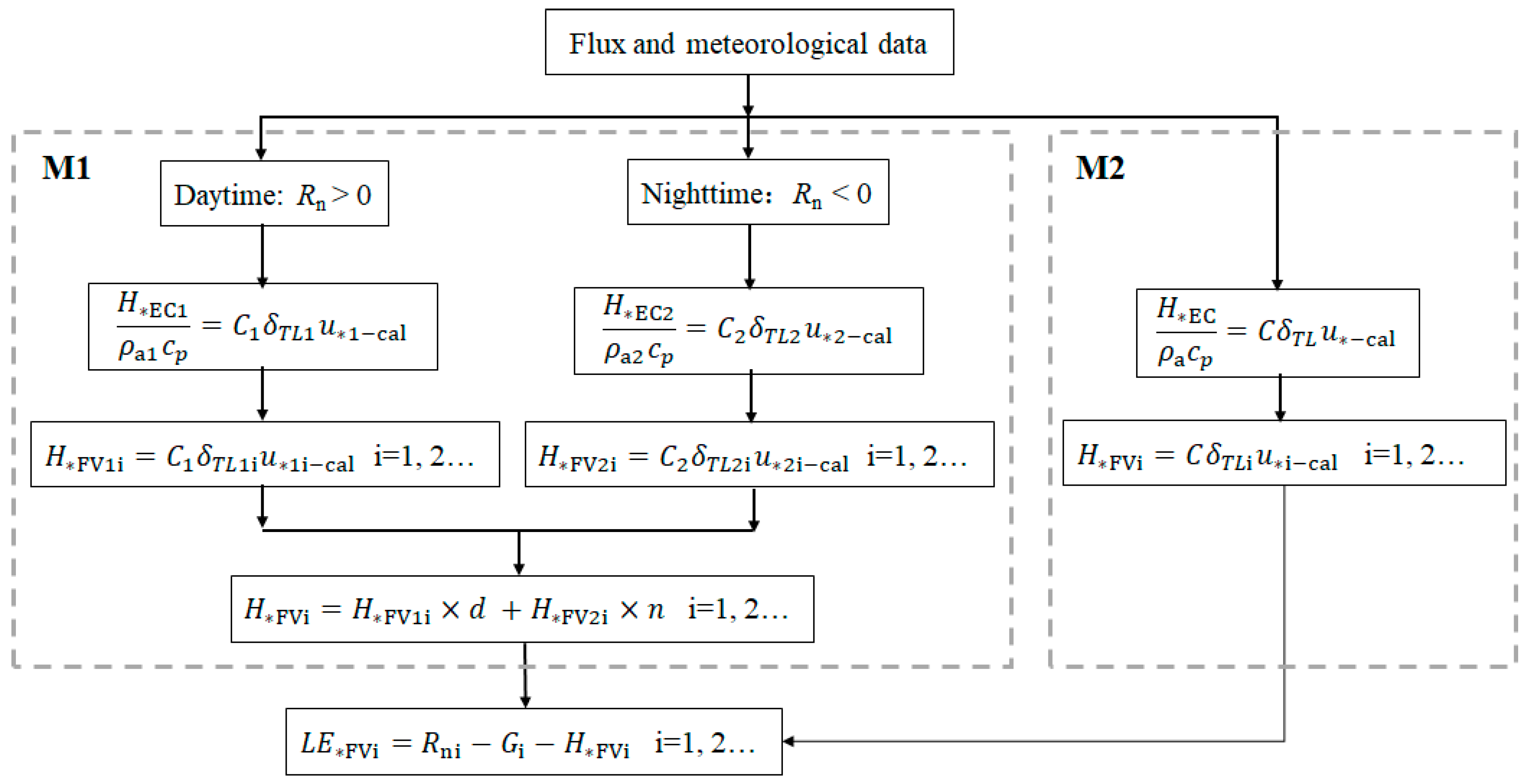
Method 1 (M1): First, all half-hourly data were divided into daytime (net radiation (Rn) > 0) and nighttime groups (Rn < 0), and the mean values were calculated. Second, constants C1 and C2 were determined from the linear relationship between the half-daily mean standard deviation of low-frequency temperature, friction velocity, and the sensible heat flux observed by the EC system (and corrected for energy balance closure; see Section 2.4) for daytime and nighttime, respectively.
H E C ρ a 1 c p = C 1 δ T L 1 u 1 c a l         R n > 0
H E C ρ a 2 c p = C 2 δ T L 2 u 2 c a l         R n < 0
where δ T L 1 and δ T L 2 are the half-daily mean standard deviation of low-frequency (~1 Hz) temperature (K) for daytime and nighttime, while u∗1−cal and u∗2−cal are the half-daily mean friction velocity (m s−1) for daytime and nighttime, recalculated using the wind speed profile formula under neutral stratification, which is given as follows [26].
u ¯ u c a l = 1 k ln z d z 0
where u ¯ is the half-hourly wind speed (m s−1) observed by the microclimate system (except for the two grassland sites, where wind speed was observed by the three-dimensional ultrasonic anemometer), d is the zero-plane displacement (m), taken as 2/3 of the canopy height according to empirical relationships, and z0 is the roughness length (m), taken as 0.1 times the canopy height according to empirical relationships [27]. Third, constants C1 and C2 were substituted into the calculations to estimate the half-daily mean sensible heat flux at daytime and nighttime, respectively. Finally, the daily mean sensible heat flux for each site was estimated based on the duration weights of daytime and nighttime.
H F V d = C 1 ρ a 1 c p δ T L 1 u 1 c a l         R n > 0
H F V n = C 2 ρ a 2 c p δ T L 2 u 2 c a l         R n < 0
H F V = H F V d × d + H F V n × n
where H F V d and H F V n are the half-daily mean sensible heat flux estimated for daytime and nighttime (W m−2), H F V is the daily mean estimated sensible heat flux, d is the proportion of daytime duration, and n is the proportion of nighttime duration.
Method 2 (M2): Similar to M1, but the constant was determined using the daily mean standard deviation of low-frequency temperature, friction velocity and the corrected sensible heat flux (see Figure 2).
Latent heat flux was indirectly estimated with the calculated daily mean sensible heat flux based on the energy balance equation.
L E F V = R n G H F V
where L E F V is the daily mean estimated latent heat flux, while G is the soil heat flux.

2.3. EC Flux Data Processing

For the two cropland sites (LC and YF), half-hourly data were calculated using online-processing software. Briefly, a double coordinate rotation was used to remove tilt errors [28]. The Webb–Pearman–Leuning (WPL) correction was applied to remove the density effects of temperature and water vapor variations in the measured eddy flux [29]. Abnormal flux data were filtered according to the following conditions: (1) when precipitation occurred, and (2) when the sensible heat flux was lower than −100 W m−2 or higher than 300 W m−2 and the latent heat flux was lower than −200 W m−2 or higher than 600 W m−2. The daily mean flux was determined if there were 80% or more valid half-hourly flux data on that day. The overall daily data coverages for the LC and YF sites were 79% and 74%, respectively.
Data from the two grassland sites (DL and XLHT) were available from the ChinaFLUX network, and quality control and data gap-filling had already been performed on the public flux data; thus, we directly used the data for further analysis [30,31].

2.4. Energy Balance Closure Correction

There is an energy imbalance problem in EC measurements due to the exchange processes across larger scales of the heterogeneous landscape, measurement and data processing errors, or storage terms [32,33]. Energy balance closure correction was applied to the EC fluxes, which could reduce errors in establishing universal parameters and estimating the latent heat flux calculated using the estimated sensible heat flux and the energy balance equation. Generally, the sensible and latent heat fluxes measured by EC systems are underestimated, and some studies have found that the Bowen ratio from EC measurements was more accurate than that from Bowen ratio observation systems [34,35,36]. Thus, the Bowen-ratio closure method, as described by Twine et al. [36], was employed to redistribute the residual energy term back to sensible and latent heat fluxes. The specific formulas are presented below:
β = H L E
L E = R n G 1 + β
H = R n G L E
where β is the Bowen ratio, while LE and H are the latent and sensible heat flux after energy balance closure correction, respectively. Since energy balance closure correction performs better on a longer time scale [37], the correction was conducted on half-daily (divided into daytime and nighttime) and daily scales, respectively.

3. Results

3.1. Energy Balance Closure of Each Site

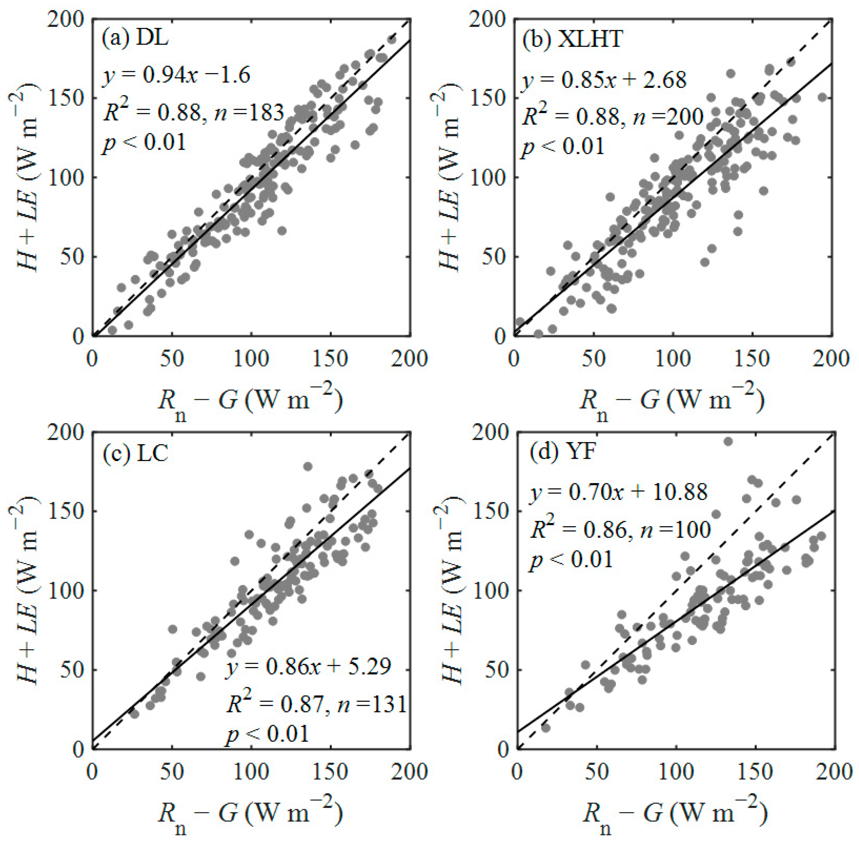
The energy balance closure analysis was conducted to evaluate the performance of EC measurements for each ecosystem. Regression analysis was performed between daily datasets of the available energy flux (RnG) and the turbulent fluxes of consumed energy (LEEC + HEC) (Figure 3). The four EC systems achieved an energy budget closure of 70% to 94% for daily averaged values. The highest energy balance closure was observed at the DL site.

3.2. Comparison of the Calculated Friction Velocity with EC Method

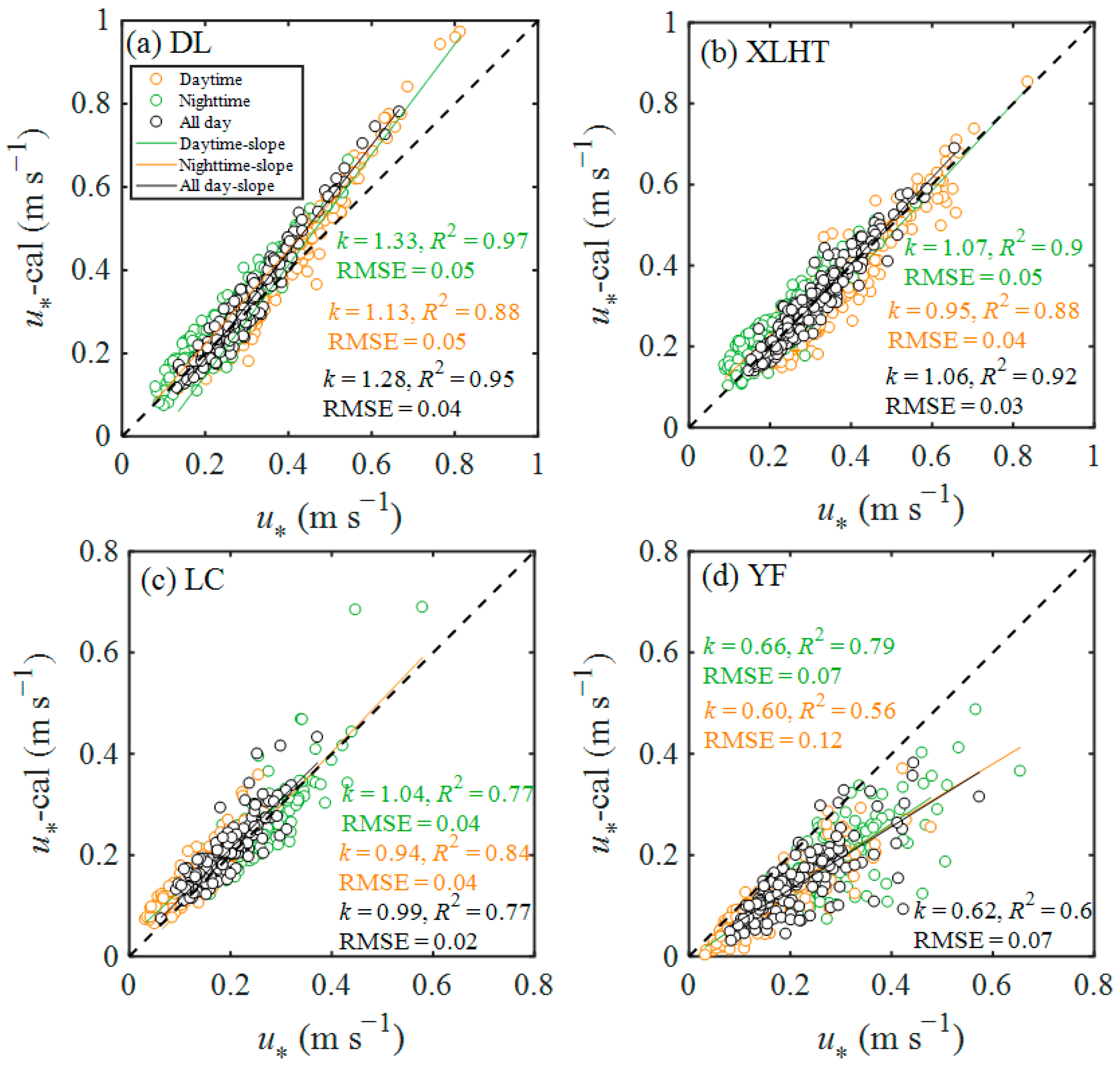
Figure 4 shows a comparison of the calculated friction velocity with EC method across three time periods. During the daytime, the friction velocity calculated for the DL, XLHT, and LC sites was higher than that obtained using the EC method. Among these, the LC site showed the smallest deviation of 4%, while the DL site had the highest deviation of 33%. Conversely, the friction velocity calculated for the YF site was lower than that obtained using the EC method, with the YF site exhibiting the greatest discrepancy, reaching a 34% reduction. At night, only the DL site displayed a higher calculated friction velocity compared to the EC measurement, showing the largest deviation of 13%. The other three sites had a lower calculated friction velocity, with the YF site showing the most significant deviation, reaching a 40% reduction. Over the entire day, the friction velocity calculated for the DL site was higher than that obtained using the EC system, showing the highest deviation of 28%. The remaining three sites had lower calculated friction velocities, with the YF site showing the most significant deviation, reaching a 38% reduction.
Overall, the XLHT and LC sites performed best in calculating friction velocity, with differences from the EC system being less than 10%. In contrast, as the measurement height of the EC system was three times higher than that of the microclimate system in the YF site, the calculation results were, as expected, greatly underestimated. The calculated friction velocity at these sites was more dispersed relative to those from EC systems, being 38% to 40% lower at the YF site. Additionally, the YF site had an R2 value below 0.8, indicating a relatively weak fit of the model to the measurement.

3.3. Comparison of Sensible Heat Flux Between EC Measurement and FV Prediction

A new FV relationship needs to be determined before applying the daily-scale FV method to estimate the sensible heat flux. With corrected EC measurements, low-frequency air temperature, and the calculated friction velocity, we determined the FV relationships of sensible heat flux using data from all sites. Figure 5 shows the sensible heat flux (H∗EC/(ρa × cp)) as a function of the standard deviation of temperature and friction velocity (σTL × u∗-cal) for (a) daytime, (b) nighttime, and (c) all day. The constants for daytime, nighttime, and all day were 0.0884, −0.0274, and 0.0283, respectively.
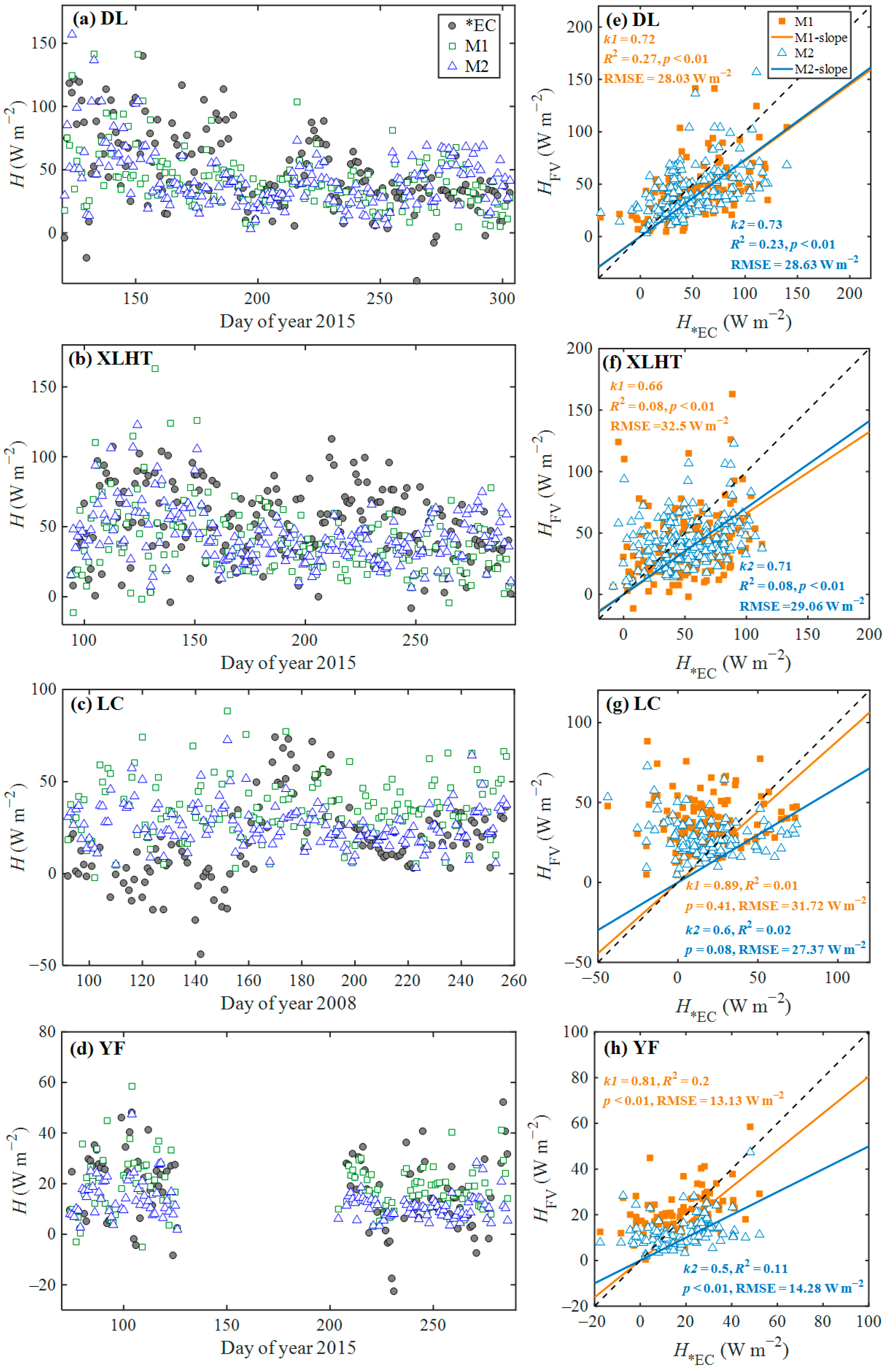
With the procedure described in Figure 2 and the estimated constants presented in Section 3.3, two methods were used to estimate sensible heat flux for the four sites on a daily scale: one calculated using constants obtained from daytime and nighttime data (M1) and the other calculated using the constant obtained from daily data (M2). As the sensible heat flux from the EC system was corrected, a regression model through the origin (HEC = A × HFV) was used to evaluate the sensible heat flux estimated by the FV method. As shown in Figure 6, the temporal variations in the sensible heat flux were captured by the FV method in some periods (e.g., DOY 200 to 303 at the DL site). However, poor agreement was observed between the daily estimated sensible heat flux of the FV and EC methods across all sites, with slopes of 0.50~0.81, determination coefficients (R2) of 0.01~0.27, and root mean square error (RMSE) of 13.13~32.50 W m−2, indicating underestimation of sensible heat flux calculated by both M1 and M2. The largest underestimation occurred at the YF site. Note that for the LC site, the sensible heat flux calculated using both M1 and M2 did not pass the significance test when compared with the EC system. Additionally, negative sensible heat flux was observed by EC systems over cropland sites, whereas the sensible heat flux estimated by the FV method was positive. These phenomena resulted in worse performance compared to EC measurements, especially for the LC site, as about 18% of the daily flux was negative.
Comparing these two calculation methods, for the two grassland sites, the sensible heat flux calculated by M2 showed better performance in estimation than that by M1 compared to EC results, while the comparison of the two methods from the two cropland sites was the opposite.

3.4. Comparison of Latent Heat Flux Between EC Measurement and FV Prediction

As shown in Figure 7, overall, the temporal variations in the latent heat flux were captured by the FV method. Relatively good agreement was observed between the daily estimated latent heat flux from the FV and EC methods across all sites, with slopes of 0.78~1.18, R2 of 0.44~0.88, and RMSE of 13.13~32.50 W m−2. Among the four sites, the latent heat flux estimated by M1 and M2 at the DL and XLHT sites was overestimated, while the LC site showed underestimation. The estimated latent heat flux at the YF site was the best, with slopes of 0.98~1.04 and R2 of 0.88. Latent heat flux estimated by the FV method over cropland sites showed better performance than that at grassland sites.
Comparing these two calculation methods, the latent heat flux calculated by M1 and M2 was very close at the two grassland sites. The latent heat flux calculated by M2 was better than that calculated by M1 at the LC site, while the result at the YF site was the opposite.

4. Discussion

4.1. FV-Estimated Sensible Heat Flux

In this study, the FV-estimated sensible heat flux was lower than that measured by the EC system in both grassland and cropland ecosystems. This finding is consistent with results from previous studies, where the FV-calculated sensible heat flux exhibited a high degree of agreement with EC measurements under unstable atmospheric conditions, with regression slopes of 0.79~1.03 and RMSE of 25~44.84 W m−2 [3,22,38,39,40]. However, our estimated results were more significantly underestimated, mainly due to the following two reasons. One reason is the estimation of friction velocity. The underestimated friction velocity in cropland ecosystems was consistent with the underestimated FV-estimated sensible heat flux, indicating that relative errors may be transferred to the calculation of sensible heat flux. This finding is similar to the result of French et al. [19], who concluded that the underestimated friction velocity calculated from wind speed data brought about 16%~28% underestimations for the FV-estimated sensible heat flux. In addition, special phenomena such as negative sensible heat flux, which primarily occur during the crop-growing season due to irrigation [3], are particularly evident at cropland sites (LC and YF).

4.2. FV-Estimated Latent Heat Flux

The FV method can directly calculate latent heat flux, but several studies have found that the results for latent heat flux are not as effective as those for sensible heat flux, which is attributed to the heterogeneity of sources and sinks for sensible and latent heat fluxes at the surface [13,41]. Therefore, some studies combine calculated sensible heat flux to estimate latent heat flux, achieving better results than directly using the FV method [3,40]. We also indirectly estimated latent heat flux based on the energy balance equation and the sensible heat flux calculated using the new FV method. The findings of this study indicate that the latent heat flux calculated using the daily-scale FV method performed well, which is similar to other studies showing good agreement between calculated latent heat flux under unstable conditions and EC measurements with slopes of 0.76~1.31 and RMSE of 23.12~44.77 W m−2 [3,16,17,22,38,39,40]. However, there is an overestimation of latent heat flux at grassland sites, whereas the results at cropland sites are very close to those obtained by the EC system, suggesting better performance over cropland sites than over grassland sites. This result is consistent with the findings of Hsieh et al. [3].

4.3. Outlook

It is surprising that the estimated latent heat flux performed better than the sensible heat flux over both grassland and cropland ecosystems in the present study, which differs from other literature results [13,42]. However, a study by Hsieh et al. [3] has also demonstrated a similar result over an irrigated paddy rice field, as the surface sources/sinks for water vapor were more homogeneous than those for sensible heat. Although the latent heat flux was estimated using the energy balance equation, the energy distribution of surface turbulent fluxes may influence the estimations in this study, that is, the compensation effects in the residual energy balance. For grassland ecosystems, the latent heat flux was approximately half of the sensible heat flux. Therefore, the accuracy of the estimated latent heat flux depends on that of the sensible heat flux. As the calculated sensible heat flux for the DL and XLHT sites was underestimated, the latent heat flux was overestimated. The compensation effects were more obvious in cropland ecosystems, as the latent heat flux was significantly higher than the sensible heat flux. Particularly at the YF site, even though the calculated sensible heat flux was underestimated, the latent heat flux showed good agreement with EC measurements. Thus, the daily-scale FV method may be more suitable for ecosystems where more net energy is allocated to evapotranspiration rather than surface heating. Subsequently, attempts can be made to improve the accuracy of sensible heat flux estimation by refining the algorithm for calculating friction velocity and developing strategies to handle negative sensible heat flux.
Two advantages can be found in the new FV method to estimate sensible and latent heat fluxes in this study. First, compared to the traditional FV methods or some studies obtaining the FV relations with high-frequency air temperature measurements by fine-wire thermocouples, the estimations from the daily-scale FV method are fully independent from EC systems with low-frequency microclimate measurements, which greatly reduces the cost of expenses and can be applied to more sites [3,17,40]. In fact, focusing on daily estimations of sensible and latent heat fluxes in the current paper is a compromise due to the use of low-frequency data. This differs from many studies that use the traditional FV method to obtain predictions on a half-hourly scale under unstable conditions [38,40]. The half-daily-scale method yields better estimations of sensible and latent heat fluxes than the daily-scale method, suggesting that estimations using the daily-scale FV method still depend on atmospheric stability classification. Additionally, simple universal constants were obtained with the relatively uniform surfaces (grassland and cropland ecosystems), which was also different from some studies that obtain the similarity constants with different surfaces [3,5]. Moving forward, testing the method across a wide range of site data will be the next step.

5. Conclusions

The present study tested the daily-scale FV method that depends on low-frequency air temperature measurements to predict sensible and latent heat fluxes over grassland and cropland ecosystems. Our results suggest the following:
  • For the four sites, the sensible heat flux estimations showed poor correlation with EC measurements, primarily due to the occurrence of negative flux values. However, the latent heat flux estimations demonstrated reasonable agreement with EC measurements, indicating that the FV method provided more accurate latent heat flux estimation than sensible heat flux estimation.
  • Even though the estimated sensible heat flux was underestimated across both grassland and cropland ecosystems, the estimated latent heat flux over cropland sites was better than that over grassland sites, indicating that the daily-scale FV method may be more appropriate for ecosystems where more surface energy is used for evapotranspiration.
  • Compared to the two daily-scale FV methods, employing fitting constants derived from the half-daily scale yielded better results for both sensible and latent heat flux calculations than those obtained from the daily-scale method.
  • The constants of the daily-scale FV relations for daytime (0.0884) and nighttime (−0.0274) are recommended for homogeneous surfaces.

Author Contributions

Conceptualization, X.L.; methodology, X.L., Y.P. and Y.X.; formal analysis, J.X., Y.P. and L.H.; resources, M.Z. and W.X.; data curation, M.Z. and W.X.; writing—original draft preparation, Y.X. and J.X.; writing—review and editing, Y.X., J.X. and M.Z.; visualization, Y.X. and J.X.; supervision, M.Z.; funding acquisition, Y.X. All authors have read and agreed to the published version of the manuscript.

Funding

This research was supported by the Natural Science Foundation of Guangxi for Young Scholars (2024GXNSFBA010230) and the Open Research Fund of Key Laboratory of Ecosystem Carbon Source and Sink, China Meteorological Administration (ECSS-CMA202307).

Institutional Review Board Statement

Not applicable.

Informed Consent Statement

Not applicable.

Data Availability Statement

Some of sites (DL and XLHT) data are downloaded from the ChinaFLUX network, others are contained within the article, further inquiries can be directed to the corresponding author.

Conflicts of Interest

The authors declare no conflicts of interest.

References

  1. Trenberth, K.E.; Fasullo, J.T.; Kiehl, J. Earth’s global energy budget. Bull. Am. Meteorol. Soc. 2009, 90, 311–324. [Google Scholar] [CrossRef]
  2. Wild, M.; Folini, D.; Schär, C.; Loeb, N.; Dutton, E.G.; König-Langlo, G. The global energy balance from a surface perspective. Clim. Dyn. 2013, 40, 3107–3134. [Google Scholar] [CrossRef]
  3. Hsieh, C.I.; Lai, M.C.; Hsia, Y.J.; Chang, T.J. Estimation of sensible heat, water vapor, and CO2 fluxes using the flux-variance method. Int. J. Biometeorol. 2008, 52, 521–533. [Google Scholar] [CrossRef]
  4. Foken, T.; Aubinet, M.; Leuning, R. The eddy covariance method. In Eddy Covariance: A Practical Guide to Measurement and Data Analysis; Springer: Dordrecht, The Netherlands, 2011; pp. 1–19. [Google Scholar]
  5. Fischer, M.; Katul, G.; Noormets, A.; Pozníková, G.; Domec, J.C.; Orság, M.; Žalud, Z.; Trnka, M.; King, J.S. Merging flux-variance with surface renewal methods in the roughness sublayer and the atmospheric surface layer. Agric. For. Meteorol. 2023, 342, 109692. [Google Scholar] [CrossRef]
  6. Billesbach, D.P.; Arkebauer, T.J.; Sullivan, R.C. Intercomparison of sensible and latent heat flux measurements from combined eddy covariance, energy balance, and Bowen ratio methods above a grassland prairie. Sci. Rep. 2024, 14, 21866. [Google Scholar] [CrossRef] [PubMed]
  7. Shih, C.H.; Anderson, R.G.; Skaggs, T.H.; Juang, J.Y.; Chen, Y.Y.; Jang, Y.S.; Gu, R.Y.; Huang, C.Y.; Lo, M.H. Challenges and limitations of applying the flux variance similarity (FVS) method to partition evapotranspiration in a montane cloud forest. Agric. For. Meteorol. 2025, 362, 110391. [Google Scholar] [CrossRef]
  8. Anderson, D.E.; Verma, S.B.; Rosenberg, N.J. Eddy correlation measurements of CO2, latent heat, and sensible heat fluxes over a crop surface. Bound. Layer Meteorol. 1984, 29, 263–272. [Google Scholar] [CrossRef]
  9. Lee, X.; Massman, W.; Law, B. (Eds.) Handbook of Micrometeorology: A Guide for Surface Flux Measurement and Analysis; Springer Science & Business Media: Berlin/Heidelberg, Germany, 2004; Volume 29. [Google Scholar]
  10. Baldocchi, D. How eddy covariance flux measurements have contributed to our understanding of Global Change Biology. Glob. Change Biol. 2020, 26, 242–260. [Google Scholar] [CrossRef]
  11. Baldocchi, D. Measuring fluxes of trace gases and energy between ecosystems and the atmosphere-the state and future of the eddy covariance method. Glob. Change Biol. 2014, 20, 3600–3609. [Google Scholar] [CrossRef]
  12. Wilson, K.; Goldstein, A.; Falge, E.; Aubinet, M.; Baldocchi, D.; Berbigier, P.; Bernhofer, C.; Ceulemans, R.; Dolman, H.; Field, C.; et al. Energy balance closure at FLUXNET sites. Agric. For. Meteorol. 2002, 113, 223–243. [Google Scholar] [CrossRef]
  13. Katul, G.; Goltz, S.M.; Hsieh, C.I.; Cheng, Y.; Mowry, F.; Sigmon, J. Estimation of surface heat and momentum fluxes using the flux-variance method above uniform and non-uniform terrain. Bound. Layer Meteorol. 1995, 74, 237–260. [Google Scholar] [CrossRef]
  14. De Bruin, H.A.R.; Hartogensis, O.K. Variance method to determine turbulent fluxes of momentum and sensible heat in the stable atmospheric surface layer. Bound. Layer Meteorol. 2005, 116, 385–392. [Google Scholar] [CrossRef]
  15. Tillman, J.E. The indirect determination of stability, heat and momentum fluxes in the atmospheric boundary layer from simple scalar variables during dry unstable conditions. J. Appl. Meteorol. Climatol. 1972, 11, 783–792. [Google Scholar] [CrossRef]
  16. Guo, X.; Zhang, H.; Cai, X.; Kang, L.; Zhu, T.; Leclerc, M.Y. Flux-variance method for latent heat and carbon dioxide fluxes in unstable conditions. Bound. Layer Meteorol. 2009, 131, 363–384. [Google Scholar] [CrossRef]
  17. Wang, S.; Zhang, Y.; Lü, S.; Liu, H.; Shang, L. Estimation of turbulent fluxes using the flux-variance method over an alpine meadow surface in the eastern Tibetan Plateau. Adv. Atmos. Sci. 2013, 30, 411–424. [Google Scholar] [CrossRef]
  18. Choi, T.; Hong, J.; Kim, J.; Lee, H.; Asanuma, J.; Ishikawa, H.; Tsukamoto, O.; Zhiqiu, G.; Ma, Y.; Ueno, K.; et al. Turbulent exchange of heat, water vapor, and momentum over a Tibetan prairie by eddy covariance and flux variance measurements. J. Geophys. Res. Atmos. 2004, 109, D21106. [Google Scholar] [CrossRef]
  19. French, A.N.; Alfieri, J.G.; Kustas, W.P.; Prueger, J.H.; Hipps, L.E.; Chávez, J.L.; Evett, S.R.; Howell, T.A.; Gowda, P.H.; Hunsaker, D.J.; et al. Estimation of surface energy fluxes using surface renewal and flux variance techniques over an advective irrigated agricultural site. Adv. Water Resour. 2012, 50, 91–105. [Google Scholar] [CrossRef]
  20. Wesson, K.H.; Katul, G.; Lai, C.T. Sensible heat flux estimation by flux variance and half-order time derivative methods. Water Resour. Res. 2001, 37, 2333–2343. [Google Scholar] [CrossRef]
  21. Castellvi, F.; Martínez-Cob, A. Estimating sensible heat flux using surface renewal analysis and the flux variance method: A case study over olive trees at Sástago (NE of Spain). Water Resour. Res. 2005, 41, W09422. [Google Scholar] [CrossRef]
  22. Buttar, N.A.; Yongguang, H.; Chuan, Z.; Tanny, J.; Ullah, I.; Aleem, M. Height effect of air temperature measurement on sensible heat flux estimation using flux variance method. Pak. J. Agric. Sci. 2019, 56, 793–800. [Google Scholar]
  23. You, C.; Wang, Y.; Chen, S. A dataset of carbon and water fluxes of the typical grasslands in Duolun County, Inner Mongolia during 2006–2015. Chin. Sci. Data 2023, 8, 1–11. [Google Scholar] [CrossRef]
  24. Wang, Y.; You, C.; Chen, S. A dataset of carbon and water fluxes of mowing grasslands in Xilinhot, Inner Mongolia during 2006–2015. Chin. Sci. Data 2023, 8, 1–10. [Google Scholar] [CrossRef]
  25. De Bruin, H.A.R.; Kohsiek, W.; Van Den Hurk, B.J.J.M. A verification of some methods to determine the fluxes of momentum, sensible heat, and water vapour using standard deviation and structure parameter of scalar meteorological quantities. Bound. Layer Meteorol. 1993, 63, 231–257. [Google Scholar] [CrossRef]
  26. Lee, X. Fundamentals of Boundary-Layer Meteorology; Springer: Cham, Switzerland, 2018; Volume 256. [Google Scholar]
  27. Maki, T. Interrelationships between zero-plane displacement, aerodynamic roughness length and plant canopy height. J. Agric. Meteorol. 1975, 31, 7–15. [Google Scholar] [CrossRef]
  28. Aubinet, M.; Vesala, T.; Papale, D. Eddy Covariance: A Practical Guide to Measurement and Data Analysis; Springer Science & Business Media: Berlin/Heidelberg, Germany, 2012. [Google Scholar]
  29. Webb, E.K.; Pearman, G.I.; Leuning, R. Correction of flux measurements for density effects due to heat and water vapour transfer. Q. J. R. Meteorol. Soc. 1980, 106, 85–100. [Google Scholar] [CrossRef]
  30. You, C.; Wang, Y.; Chen, S. A dataset of carbon and water fluxes of the typical grasslands in Duolun County, Inner Mongolia during 2006–2015. Sci. Data Bank 2023, 8, 1–11. [Google Scholar] [CrossRef]
  31. Wang, Y.; You, C.; Chen, S. A dataset of carbon and water fluxes of mowing grasslands in Xilinhot, Inner Mongolia during 2006–2015. Sci. Data Bank 2023, 8, 1–10. [Google Scholar] [CrossRef]
  32. Foken, T. The energy balance closure problem: An overview. Ecol. Appl. 2008, 18, 1351–1367. [Google Scholar] [CrossRef] [PubMed]
  33. Leuning, R.; van Gorsel, E.; Massman, W.J.; Isaac, P.R. Reflections on the surface energy imbalance problem. Agric. For. Meteorol. 2012, 156, 65–74. [Google Scholar] [CrossRef]
  34. Barr, A.G.; King, K.M.; Gillespie, T.J.; Den Hartog, G.; Neumann, H.H. A comparison of Bowen ratio and eddy correlation sensible and latent heat flux measurements above deciduous forest. Bound. Layer Meteorol. 1994, 71, 21–41. [Google Scholar] [CrossRef]
  35. Blanken, P.D.; Black, T.A.; Yang, P.C.; Neumann, H.H.; Nesic, Z.; Staebler, R.; Hartog, G.; Novak, M.D.; Lee, X. Energy balance and canopy conductance of a boreal aspen forest: Partitioning overstory and understory components. J. Geophys. Res. Atmos. 1997, 102, 28915–28927. [Google Scholar] [CrossRef]
  36. Twine, T.E.; Kustas, W.P.; Norman, J.M.; Cook, D.R.; Houser, P.; Meyers, T.P.; Prueger, J.H.; Starks, P.J.; Wesely, M.L. Correcting eddy-covariance flux underestimates over a grassland. Agric. For. Meteorol. 2000, 103, 279–300. [Google Scholar] [CrossRef]
  37. Wohlfahrt, G.; Haslwanter, A.; Hörtnagl, L.; Jasoni, R.L.; Fenstermaker, L.F.; Arnone III, J.A.; Hammerle, A. On the consequences of the energy imbalance for calculating surface conductance to water vapour. Agric. For. Meteorol. 2009, 149, 1556–1559. [Google Scholar] [CrossRef]
  38. Gao, Z.; Bian, L.; Chen, Z.; Sparrow, M.; Zhang, J. Turbulent variance characteristics of temperature and humidity over a non-uniform land surface for an agricultural ecosystem in China. Adv. Atmos. Sci. 2006, 23, 365–374. [Google Scholar] [CrossRef]
  39. Li, Y.; Lu, P. Estimation of surface fluxes using flux-variance method over alpine meadow on east edges of Tibetan Plateau. J. Meteorol. Environ. 2014, 30, 134–140. [Google Scholar]
  40. Buttar, N.A.; Hu, Y.; Tanny, J.; Raza, A.; Niaz, Y.; Khan, M.I.; Saddique, N.; Sarwar, A.; Azeem, A.; Ahmed, F.; et al. Estimation of sensible and latent heat fluxes using flux variance method under unstable conditions: A case study of tea plants. Atmosphere 2022, 13, 1545. [Google Scholar] [CrossRef]
  41. Padro, J. An investigation of flux-variance methods and universal functions applied to three land-use types in unstable conditions. Bound. Layer Meteorol. 1993, 66, 413–425. [Google Scholar] [CrossRef]
  42. Moriwaki, M.; Kanda, M. Local and global similarity in turbulent transfer of heat, water vapor, and CO2 in the dynamic convective sublayer over a suburban area. Bound. Layer Meteorol. 2006, 120, 163–179. [Google Scholar] [CrossRef]
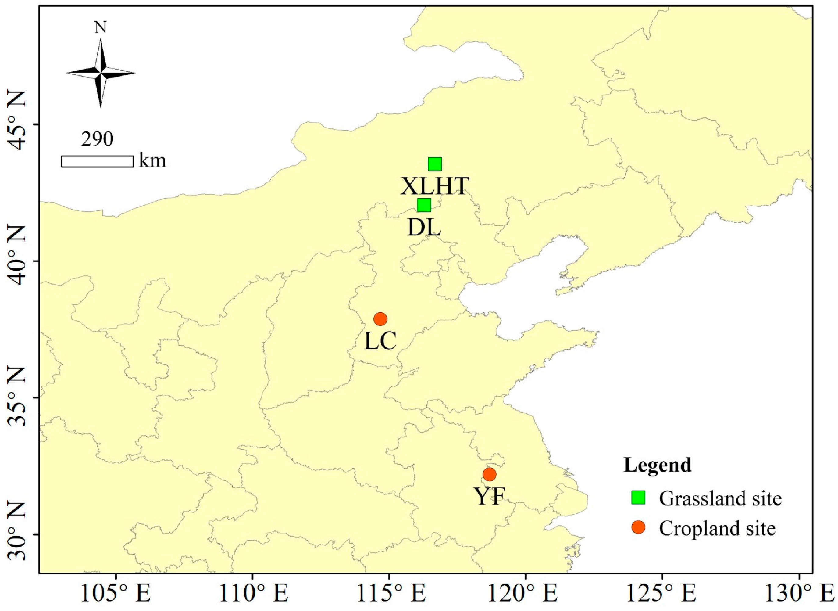
Figure 1. Geographic location map.
Atmosphere 16 01030 g001
Figure 2. Flowchart for estimating sensible and latent heat fluxes using the daily-scale FV method.
Atmosphere 16 01030 g002
Figure 3. Relationship between daily average turbulent energy flux (H + LE) and available energy (RnG) for each site: (a) DL; (b) XLHT; (c) LC; (d) YF. The linear equation, along with the associated coefficients of determination (R2), number of data (n) and the statistically significant value are provided.
Atmosphere 16 01030 g003
Figure 4. Comparison of friction velocity u observed by EC systems with calculated friction velocity u∗-cal for each site: (a) DL; (b) XLHT; (c) LC; (d) YF. The slopes of linear regression (k) with the intercept forced to zero, R2 and the root mean square error (RMSE), are provided.
Atmosphere 16 01030 g004
Figure 5. Sensible heat flux measured by EC systems (H∗EC/(ρa × cp)) as a function of standard deviation of temperature and friction velocity (σTL × u∗-cal) for (a) daytime, (b) nighttime, and (c) all day.
Atmosphere 16 01030 g005
Figure 6. Comparisons of daily sensible heat flux measured by the EC system (H∗EC) and calculated by two daily-scale FV methods (HFV). (ad) Time series for DL, XLHT, LC, and YF sites, (eh) 1:1 plot for DL, XLHT, LC, and YF sites. The k with the intercept forced to zero, R2, the statistically significant value, and RMSE are provided.
Atmosphere 16 01030 g006
Figure 7. Comparisons of daily latent heat flux measured by the EC system (LE∗EC) and calculated by two daily-scale FV methods (LEFV). (ad) Time series for DL, XLHT, LC, and YF sites, (eh) 1:1 plot for DL, XLHT, LC, and YF sites. The k with the intercept forced to zero, R2, the statistically significant value, and RMSE are provided.
Atmosphere 16 01030 g007
Table 1. Summary of site characteristics and instrumentation at four sites.
SiteDuolun (DL)Xilinhot
(XLHT)
Luancheng (LC)Yongfeng (YF)
Climatetemperatetemperatewarm temperatesubtropical monsoon
Annual mean temperature (°C)2.42.612.315.4
Annual precipitation (mm)3753495311110
Date of experiment1 May–30 October 2015 4 April–20 October 20151 April–13 September 200815 March–6 May 2015,
23 July–13 October 2015
Observation days183200166136
ecosystemgrasslandgrasslandwheat + maizewheat + rice
Canopy height (m)0.40.20.17~2.770.45~1.10
EC system
Measurement height (m)443.56
Sonic anemometerCSAT3, Campbell Scientific, Inc., Logan, UT, USACSAT3CSAT3CSAT3
CO2/H2O analyzerLi-7500, LI-COR Biosciences, Lincoln, NE, USALi-7500Li-7500Li-7500
Microclimate system
Measurement height (m)443.52
Air temperatureHMP45C (1 m), Vaisala Inc., Helsinki, FinlandHMP45C (1 m)HMP45CHMP155
Wind speed//A100R05103
Surface radiationCNR1CNR1CNR1CNR4
Soil heat flux
Measurement depth (cm)2255
Disclaimer/Publisher’s Note: The statements, opinions and data contained in all publications are solely those of the individual author(s) and contributor(s) and not of MDPI and/or the editor(s). MDPI and/or the editor(s) disclaim responsibility for any injury to people or property resulting from any ideas, methods, instructions or products referred to in the content.