Article

Mapping Ecosystem Carbon Storage in the Nanling Mountains of Guangdong Province Using Machine Learning Based on Multi-Source Remote Sensing

1
College of Resources and Environment, South China Agricultural University, Guangzhou 510640, China
2
College of Biology and Agriculture, Shaoguan University, Shaoguan 512005, China
3
North Guangdong Engineering Technology Research Center for the Efficient Utilization of Water and Soil Resources, Shaoguan 512005, China
4
Tangshan Vocational and Technical College, Tangshan 063000, China
*
Authors to whom correspondence should be addressed.
Atmosphere 2025, 16(8), 954; https://doi.org/10.3390/atmos16080954 (registering DOI)
Submission received: 25 June 2025 / Revised: 6 August 2025 / Accepted: 7 August 2025 / Published: 10 August 2025

Abstract

Accurate assessment of terrestrial ecosystem carbon storage is essential for understanding the global carbon cycle and informing climate change mitigation strategies. However, traditional estimation models face significant challenges in complex mountainous regions due to difficulties in data acquisition and high ecosystem heterogeneity. This study focuses on the Nanling Mountains in Guangdong Province, China, utilizing the Google Earth Engine (GEE) platform to integrate multi-source remote sensing data (Sentinel-1/2, ALOS, GEDI, MODIS), topographic/climatic variables, and field-collected samples. We employed machine learning models to achieve high-precision prediction and high-resolution mapping of ecosystem carbon storage while also analyzing spatial differentiation patterns. The results indicate that the Random Forest algorithm outperformed Gradient Boosting Decision Tree and Classification and Regression Tree (CART) algorithms by suppressing overfitting through dual randomization. The integration of multi-source data significantly enhanced model performance, achieving a coefficient of determination (R2) of 0.87 for aboveground biomass (AGB) and 0.65 for soil organic carbon (SOC). Integrating precipitation, temperature, and topographic variables improved SOC prediction accuracy by 96.77% compared to using optical data alone. The total carbon storage reached 404 million tons, with forest ecosystems contributing 96.7% of the total and soil carbon pools accounting for 60%. High carbon density zones (>160 Mg C/ha) were mainly concentrated in mid-elevation gentle slopes (300–700 m). The proposed integrated “optical-radar-topography-climate” framework offers a scalable and transferable solution for monitoring carbon storage in complex terrains and provides robust scientific support for carbon sequestration planning in subtropical mountain ecosystems.

1. Introduction

Terrestrial ecosystems represent the planet’s largest active carbon pool, storing approximately 2500 Pg C—three times the atmospheric carbon inventory [1]. Forest ecosystems contribute 80% of global vegetation carbon storage and 40% of soil carbon storage [2]. However, under dual pressures from land use change (e.g., deforestation, agricultural expansion) and climate change (e.g., droughts, wildfires), the carbon sink function in some regions faces significant challenges. For instance, portions of the Amazon rainforest have transitioned from carbon sinks to sources [3], underscoring the urgency of dynamic regional carbon monitoring. Subtropical forests exhibit exceptional carbon sequestration capacity (8–12 Mg C ha−1 yr−1), substantially exceeding that of temperate and boreal forests [4]. As a critical subtropical ecological zone in China, the Nanling Mountains play a vital role in regional carbon stabilization, water/soil conservation, and climate regulation [5]. Nevertheless, carbon storage assessment in this region confronts multiple challenges: topographic complexity limits comprehensive ground surveys and increases costs [6]; ecosystem heterogeneity from intermixed forests, shrublands, grasslands, and croplands complicates modeling [7]; optical remote sensing suffers from cloud interference [8]; and radar data exhibit saturation issues in vegetation structural inversion [9]. Consequently, developing robust carbon density prediction models for heterogeneous ecosystems and structurally complex vegetation is essential for high-precision carbon mapping in the Nanling Mountains.
According to IPCC guidelines [10], terrestrial carbon storage comprises aboveground, belowground, soil, and dead carbon pools. Given the minimal and unmeasurable nature of dead carbon, this study focuses on aboveground, belowground, and soil carbon storage. Aboveground carbon and belowground carbon are derived from vegetation biomass (forests, grasslands, croplands) and carbon conversion rates, making biomass estimation foundational to vegetation carbon assessment. Since the 1970s Landsat launches, optical remote sensing has advanced regional vegetation carbon studies through biomass estimation via vegetation indices. Baccini et al. quantified deforestation-driven carbon emissions using MODIS and Landsat imagery [11], while Forkel et al. revealed global spatiotemporal patterns of vegetation dynamics and carbon turnover with multi-source remote sensing [12]. However, optical data face limitations in cloudy regions due to low acquisition rates and atmospheric effects [13], necessitating supplementation by radar or LiDAR. Radar remote sensing addresses these gaps. Spaceborne LiDAR (e.g., GEDI, ICESat-2) enables direct vegetation vertical structure measurement, achieving ~80% accuracy in aboveground biomass (AGB) inversion [14]. The GEDI mission, with 1 billion global laser footprints, provides the first high-resolution (25 m) global AGB product (L4A), correlating strongly with ground data (R2 = 0.67–0.92) [15,16]. Yang et al. further demonstrated GEDI’s utility for bamboo forest AGB estimation in Yunnan (R2 = 0.87) [17]. Nevertheless, GEDI’s accuracy declines in high-density tropical/subtropical montane forests. L-band SAR (e.g., ALOS) mitigates surface roughness effects in topographically complex regions, enhancing biomass stability—particularly for tropical/subtropical forests >100 Mg ha−1 [18,19,20]. The emergence of Google Earth Engine (GEE) has enabled global-scale synergistic analysis of optical, radar, LiDAR, climatic, and topographic data. Yan et al. developed an AGB model for Taiyue Mountain, China, integrating Landsat, SAR, and field samples [21]. Machine learning algorithms have significantly improved carbon storage predictions in complex terrain through nonlinear modeling [22,23]. Singha et al. demonstrated GEE-based AGB prediction using Sentinel and GEDI data, with Random Forest outperforming other methods (R2 = 0.71) [24]. By integrating multi-source remote sensing and machine learning, GEE revolutionizes high-resolution carbon storage assessment, leveraging petabyte-scale data storage and parallel computing for efficient global analysis [25,26]. Thus, GEE-based fusion of optical and radar data offers a robust pathway for large-scale, high-precision biomass prediction.
Soil carbon constitutes two-thirds of global terrestrial carbon pools but exhibits high spatial heterogeneity driven by climate, vegetation, topography, and human activities [27]. Traditional soil organic carbon (SOC) mapping relies on spatial interpolation of soil samples, yielding errors up to 30% in mountains due to sparse sampling [28]. Digital soil mapping has recently enhanced SOC prediction by integrating remote sensing, terrain indices, and machine learning. The global SoilGrids dataset (250 m resolution) employs quantile regression forests, achieving a root mean square error (RMSE) of 36.48 g kg−1 [29]. Multi-source fusion has since become mainstream: Vaudour et al. attained R2 = 0.56 for SOC using Sentinel-2 [30]; Schillaci et al. reached R2 = 0.63–0.69 with Landsat, topography, and soil texture [31]; Zhou et al. improved SOC accuracy by 29.1% using Landsat/Sentinel fusion [32]; Ho et al. achieved R2 = 0.71 for tropical forests via deep learning with Sentinel-2, ALOS, topography, and climate data [33]. Machine learning further enables high-resolution SOC mapping [34], yet accuracy remains challenging in intensively managed farmland ecosystems.
The Nanling Mountains serve as a key water conservation area for the Pearl River Basin. Their complex topography and high biodiversity render them critical for studying the responses of subtropical mountain carbon cycles to climate change. Moreover, their carbon sink function is indispensable for achieving Guangdong’s “dual carbon” goals. This study presents a comprehensive assessment of ecosystem carbon storage within the Nanling Mountains of Guangdong Province, China. Leveraging the GEE cloud computing platform, we integrated multi-source remote sensing data with machine learning algorithms to generate the 30 m high-resolution carbon storage map for this ecologically significant subtropical mountainous region. We developed a novel cloud-based analytical framework based on the synergistic fusion of “Optical-Radar-Terrain-Climate” data sources. This integrated approach provides critical case-specific parameters for refining carbon cycle models in subtropical mountainous ecosystems.

2. Data and Methods

2.1. Study Area

The Nanling Mountains in Guangdong Province are located at 24–25.5° N and 112–115.5° E, covering an area of approximately 58,000 km2, including Shaoguan, Qingyuan, and other cities, which are the core component of the Nanling Mountains. The region is dominated by mid to low mountains, with an altitude range of 500–1902 m, and steep slopes (>25°) account for 35%, forming a complex geomorphic pattern [35]. The climate is subtropical monsoon, with an average annual temperature of 18–22 °C, annual precipitation of 1500–2000 mm, and the rainy season (April–September) concentrates 70% of annual precipitation. These favorable hydrothermal conditions provide an ideal environment for vegetation growth. These distinctive features establish the Nanling Mountains as a natural laboratory for studying carbon cycling in subtropical mountainous ecosystems and offer a representative test site for multi-source remote sensing-based carbon storage assessment.

2.2. Data and Sources

This study utilized a comprehensive suite of datasets to capture the biophysical and climatic drivers of ecosystem carbon storage (Table 1). Satellite remote sensing data were accessed from the GEE platform, including Sentinel-1, Sentinel-2, MODIS, ALOS PALSAR-2, and GEDI. Sentinel-2 images were filtered using GEE’s cloud masking algorithm to select scenes with cloud cover <1%. Remaining cloud-contaminated areas were interpolated using adjacent cloud-free images, ensuring >90% valid pixel coverage across the study area. Topographic data comprised Digital Elevation Model (DEM) data and slope. Soil properties were obtained from sources such as the Harmonized World Soil Database (HWSD). Land Use/Land Cover (LULC) was derived from high-resolution classification maps. Gridded time-series meteorological data provided temperature and precipitation records. Ancillary data, including soil sampling data and vegetation sampling data, were used for model calibration and validation where available.
Field sampling data encompassed forest, grassland, and farmland ecosystems (Figure 1). Soil sampling was conducted between August and November 2022 across 693 sites, with samples collected at a standard depth of 30 cm. This dataset was supplemented with farmland quality assessment data for specific agricultural regions. Vegetation sampling utilized 2022 National Forest Inventory data, strategically integrated with GEDI-derived canopy metrics. Following rigorous quality control and outlier removal, the final vegetation dataset comprised 2029 validated plots. A total of 2722 sampling points were established after rigorous quality control and outlier removal, including 693 soil sites and 2029 vegetation plots, comprehensively covering forests, grasslands, and farmlands to represent the heterogeneous landscape of the Nanling Mountains in Guangdong Province. For soil and vegetation samples, stratified random sampling was applied separately: 70% of soil samples (515) and vegetation samples (1420) were allocated to training sets, with 30% (178 soil, 609 vegetation) to validation sets. Stratified by ecosystem type, this partitioning ensured consistent ecosystem distribution between training and validation sets. Notably, it was independent of sampling dates or seasons, avoiding biases from temporal variations.

2.3. Methods

2.3.1. Environmental Variables

Ecosystem carbon density exhibits dual dependency on natural environmental drivers and anthropogenic influences. To capture these dynamics, we extracted multi-source remote sensing variables informed by established determinants of vegetation biomass, vigor, structural attributes, soil moisture, and environmental conditions [38]. Key predictors included Sentinel-2-derived optical indices; MODIS productivity metrics; radar-derived Normalized Difference Index from Sentinel-1 and ALOS PALSAR; and topo-climatic variables (DEM data, slope, precipitation, temperature) (Table 2).
Recognizing the distinct drivers of AGB and SOC, we constructed a differentiated environmental variable library (Table 3) tailored to their unique influencing mechanisms. This library ensures optimized variable selection for modeling AGB and SOC, thereby enhancing the precision of ecosystem-scale carbon storage assessments.

2.3.2. Model Construction

We employed Random Forest, Gradient Boosting Decision Tree, and Classification and Regression Tree (CART) algorithms on the GEE platform to predict AGB and SOC. These tree-based algorithms operate on a “feature splitting-data partitioning” logic, making them well suited for regression tasks.
CART serves as the foundational algorithm, providing the binary tree structure framework for Random Forest and Gradient Boosting Decision Trees. It selects optimal split points by minimizing the sum of squared errors within nodes. Both Random Forest and Gradient Boosting Decision Trees are ensemble methods that enhance predictive performance by combining multiple CARTs but differ fundamentally in their integration strategies.
Random Forest, a widely applied ensemble method in ecology [42,43], generates multiple training subsets via bootstrap sampling with replacement from the environmental feature dataset using soil and vegetation field samples. During node splitting, each decision tree considers only a random subset of features, increasing model diversity. Nodes are split based on information gain, and the final prediction is obtained by averaging the outputs of all trees, improving stability.
Gradient Boosting Decision Trees follow a boosting framework [44]. Their core principle involves iteratively training decision trees to sequentially correct errors from previous models, combining multiple weak learners (decision trees) into a strong predictor [45]. GBDT automatically selects key variables via split gain and incorporates feature subsampling to reduce redundancy. Facing spatial heterogeneity, initial trees identify region-specific patterns through splitting rules, while subsequent trees focus on optimizing local residuals.
Models were implemented on the GEE platform using JavaScript ES5, leveraging the smile library suite—specifically smileCart for constructing CART [46], smileGradientTreeBoost for Gradient Boosting Decision Trees, and smileRandomForest for Random Forest algorithms.

2.3.3. Carbon Storage Calculation

According to the root/shoot ratio of different vegetation types and the ratio of AGB to belowground biomass (BGB) [47], and predicting the carbon conversion coefficient based on environmental variable information such as vegetation structure, vegetation carbon storage (CV) was calculated. The formula of BGB is as follows:
B G B = A G B × R
where R represents the ratio of BGB to AGB, which adopts the recommended values from IPCC [48].
C V = A G B + B G B × F
where F represents the carbon conversion coefficients.
Soil carbon storage (Cs) of different ecosystems was calculated based on the depth of 30 cm soil carbon density and soil bulk density data from the HWSD2.0. The formula is as follows:
C s = S O C × S o i l   B u l k   D e n s i t y × D e p t h
The carbon storage (Ct) in the Nanling Mountains is the sum of vegetation carbon storage and soil carbon storage. The formula is as follows:
C t = C v + C s

2.3.4. Workflow

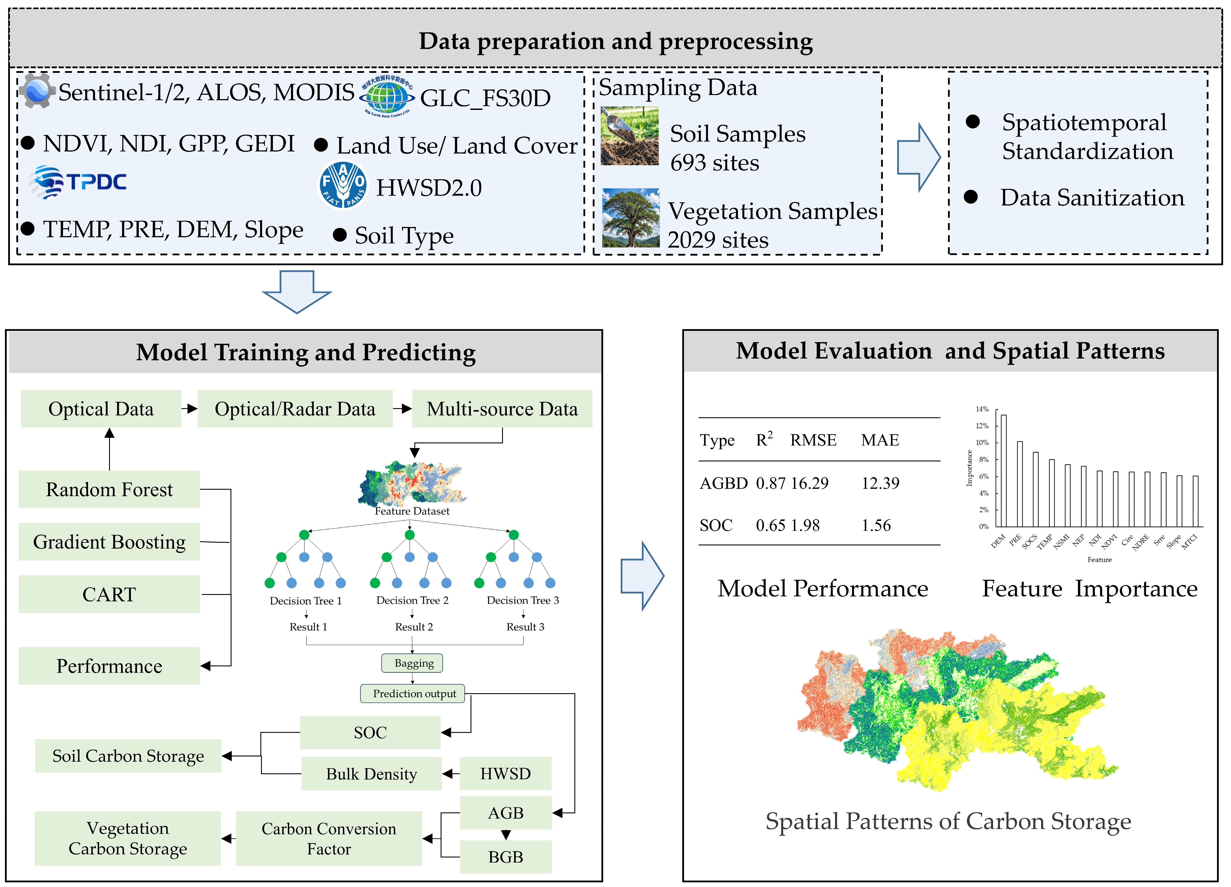
Based on the GEE platform, we integrated multi-source remote sensing, and topographic and climatic features with machine learning algorithms to achieve high-precision assessment and high-resolution mapping of carbon storage (Figure 2).
(1) Data acquisition: Obtain Sentinel-1/2 imagery from October to December 2022, GEDI L4A aboveground biomass density data, ALOS PALSAR-2 annual mosaic imagery, and MODIS vegetation gross/net primary productivity products. Supplement with gridded precipitation and temperature data, topographic factors, and Land Use/Land Cover data to comprehensively capture the heterogeneity of ecosystems in the Nanling Mountains of Guangdong Province.
(2) Feature engineering: Calculate remote sensing indices, unify the spatial reference system (WGS 1984) and spatial resolution (30 m), and fuse multi-source environmental variables to form feature datasets for AGB and SOC.
(3) Model training and prediction: Use field sample points to train machine learning models to predict AGB and SOC. Evaluate model performance through the R2, RMSE, and mean absolute error (MAE). Test different environmental variable combinations to optimize accuracy and compare the performance of different machine learning models to select the optimal model.
(4) Carbon storage calculation: Convert predicted biomass to vegetation carbon density using carbon conversion coefficients of different vegetation types. Calculate soil carbon density using predicted soil organic carbon content combined with bulk density data from the HWSD2.0. Overlay vegetation and soil carbon pools to generate the total carbon storage distribution map of the Nanling Mountains in Guangdong Province.
(5) Spatial analysis: Analyze the spatial differentiation of carbon density along altitude gradients and land cover types, and quantify the influence intensity of terrain/climate/vegetation interaction effects.

3. Results

3.1. Accuracy Assessment with Multi-Source Data

We predicted AGB and SOC using Random Forest, integrating field survey data with three progressively complex sets of environmental variables: Optical remote sensing indices only, Optical + radar remote sensing indices, Optical indices + radar indices + topo-climatic features. For model validation, 30% of the field survey plots were held out as an independent validation dataset. Prediction accuracy was rigorously evaluated using three metrics, namely, R2, MAE, and RMSE. The performance results across all variable combinations are presented in Table 4.
The results show that the fusion of multi-source data such as optical + radar + terrain/climate factors significantly improves model performance, with the highest prediction accuracy. When only optical data were used for AGB prediction, the model’s R2 was 0.79, and the RMSE and MAE were 21.03 Mg/ha and 15.66 Mg/ha, respectively. After adding radar data, the R2 increased to 0.85, and the RMSE and MAE decreased by 18.4% and 17.6%, respectively. Further fusion of terrain and climate factors optimized model accuracy. Radar data compensated for the limitations of optical data by capturing vegetation vertical structure and canopy penetration information.
When only optical data were used for SOC prediction, the R2 was 0.31, indicating limited direct sensitivity of optical bands to soil carbon. After adding radar data, the R2 increased to 0.40, and the RMSE and MAE decreased by 8.0% and 9.4%, respectively. Further fusion of precipitation, temperature, and terrain data significantly increased the R2 to 0.65, and the RMSE and MAE decreased by 17.5% and 14.3%, respectively. Terrain variables and precipitation/temperature variables jointly explained part of the spatial distribution pattern of soil carbon.

3.2. Machine Learning Model Results

3.2.1. Random Forest Algorithm

By continuously optimizing the key parameters of the Random Forest model, the number of decision trees was finally determined to be 500, the maximum number of nodes per tree was 128, the minimum number of samples per leaf node was 5, and the feature subsample size was 8.
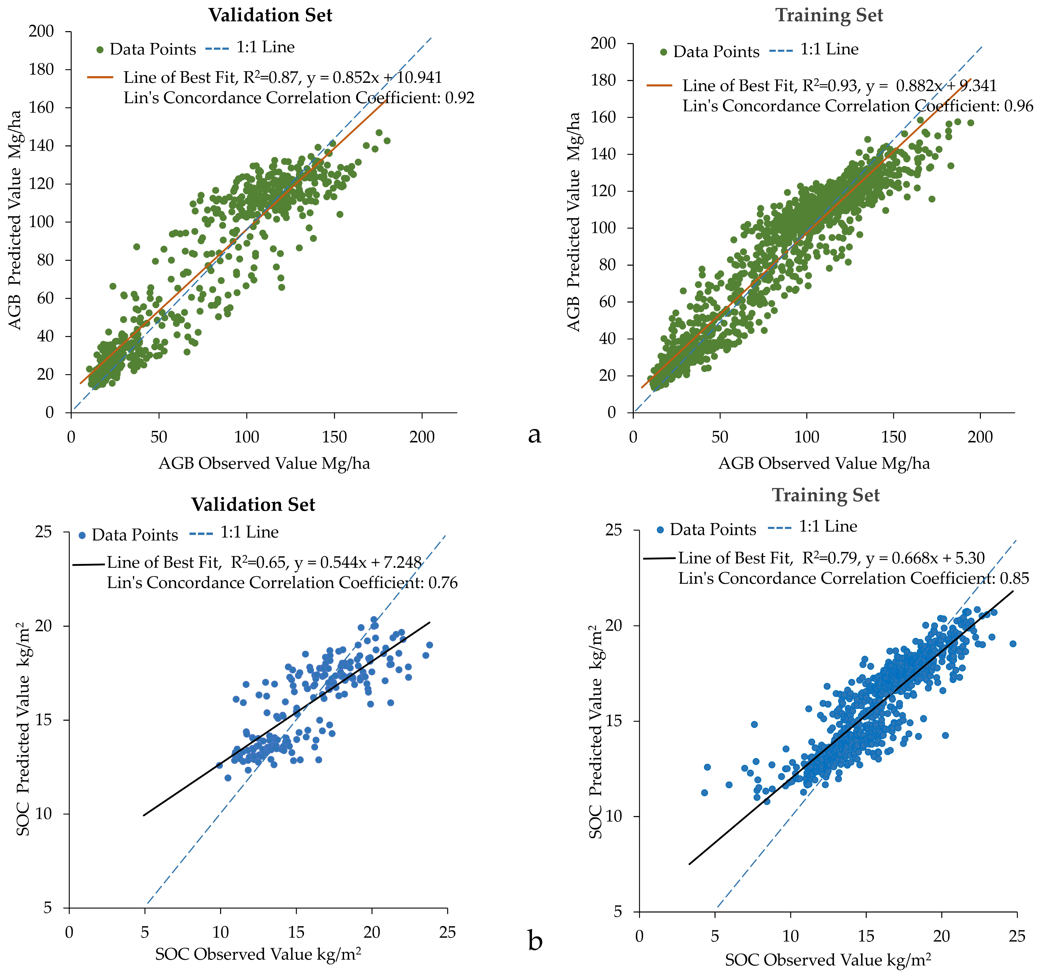
Figure 3a shows the relationship between predicted and observed values in the AGB training dataset and validation dataset. The linear regression equation for the AGB training dataset is predicted value = 0.882 × AGB observed value + 9.341, with an R2 of 0.93, RMSE of 12.41, and MAE of 9.25. The AGB validation data linear regression equation is predicted value = 0.852 × AGB observed value + 10.941, with an R2 of 0.87, RMSE of 16.29, and MAE of 12.39. This indicates that the model performs extremely well in predicting the training and validation datasets for AGB. Figure 3b shows the relationship between predicted and observed values in the SOC training dataset. The clustering of points stems from the natural concentration of SOC observed values within specific ranges (e.g., >5 kg/m2) across the sampled ecosystems in the Nanling Mountains. The linear regression equation is predicted value = 0.668 × SOC observed value + 5.30, with an R2 of 0.79, RMSE of 1.49, and MAE of 1.09. The SOC validation data linear regression equation is predicted value = 0.510 × SOC observed value + 7.8444, with an R2 of 0.65, RMSE of 1.92, and MAE of 1.50. This indicates that the model has high explanatory power for the SOC training and validation datasets.

3.2.2. Gradient Boosting Decision Tree Algorithm

By continuously optimizing the key parameters of the Gradient Boosting Decision Tree model, the number of decision trees was finally determined to be 500, the maximum number of nodes per tree was 60, the learning rate was 0.05, and the sampling rate was 0.8.
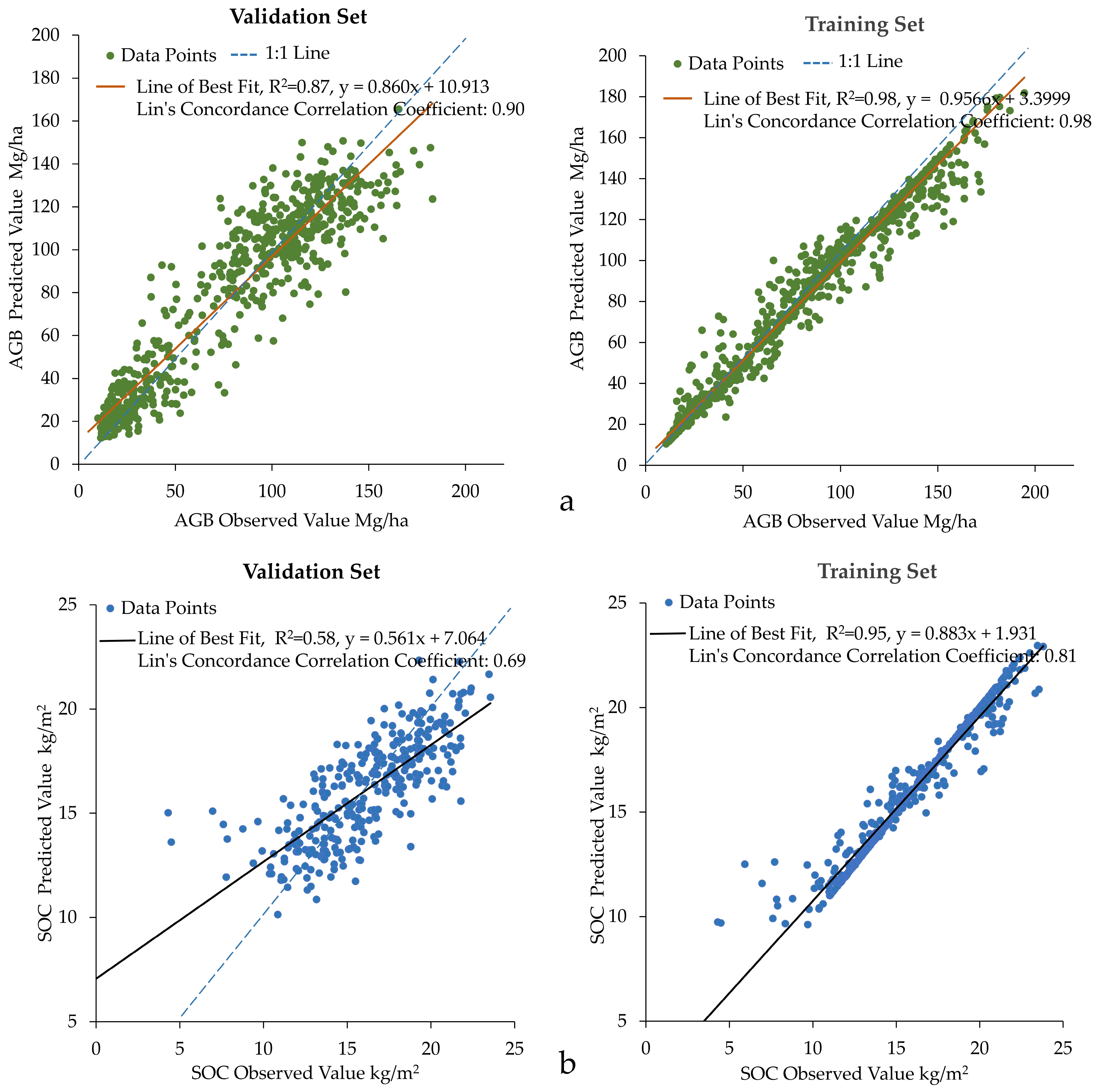
Figure 4a shows the relationship between predicted and observed values in the AGB training dataset and validation dataset. The AGB training dataset linear regression equation is predicted value = 0.957 × AGB observed value + 3.40, with an R2 of 0.98, RMSE of 6.55, and MAE of 2.97. The AGB validation data linear regression equation is predicted value = 0.860 × AGB observed value + 10.913, with an R2 of 0.87, RMSE of 16.35, and MAE of 12.21. This indicates that the model performs excellently in predicting AGB for both training and validation datasets, comparable to the Random Forest, but overfits the training dataset. Figure 4b shows the relationship between predicted and observed values in the SOC training dataset. The linear regression equation is predicted value = 0.883 × SOC observed value + 1.931, with an R2 of 0.95, RMSE of 0.70, and MAE of 0.25. The SOC validation data linear regression equation is predicted value = 0.561 × SOC observed value + 7.064, with an R2 of 0.58, RMSE of 2.15, and MAE of 1.63. This indicates that the model has high explanatory power for the SOC training dataset but overfits the training dataset and lacks stability in the validation dataset.

3.2.3. CART Algorithm

By continuously optimizing the key parameters of the CART model, the maximum number of nodes in the decision tree was finally determined to be 100, and the minimum number of samples per leaf node was 5.
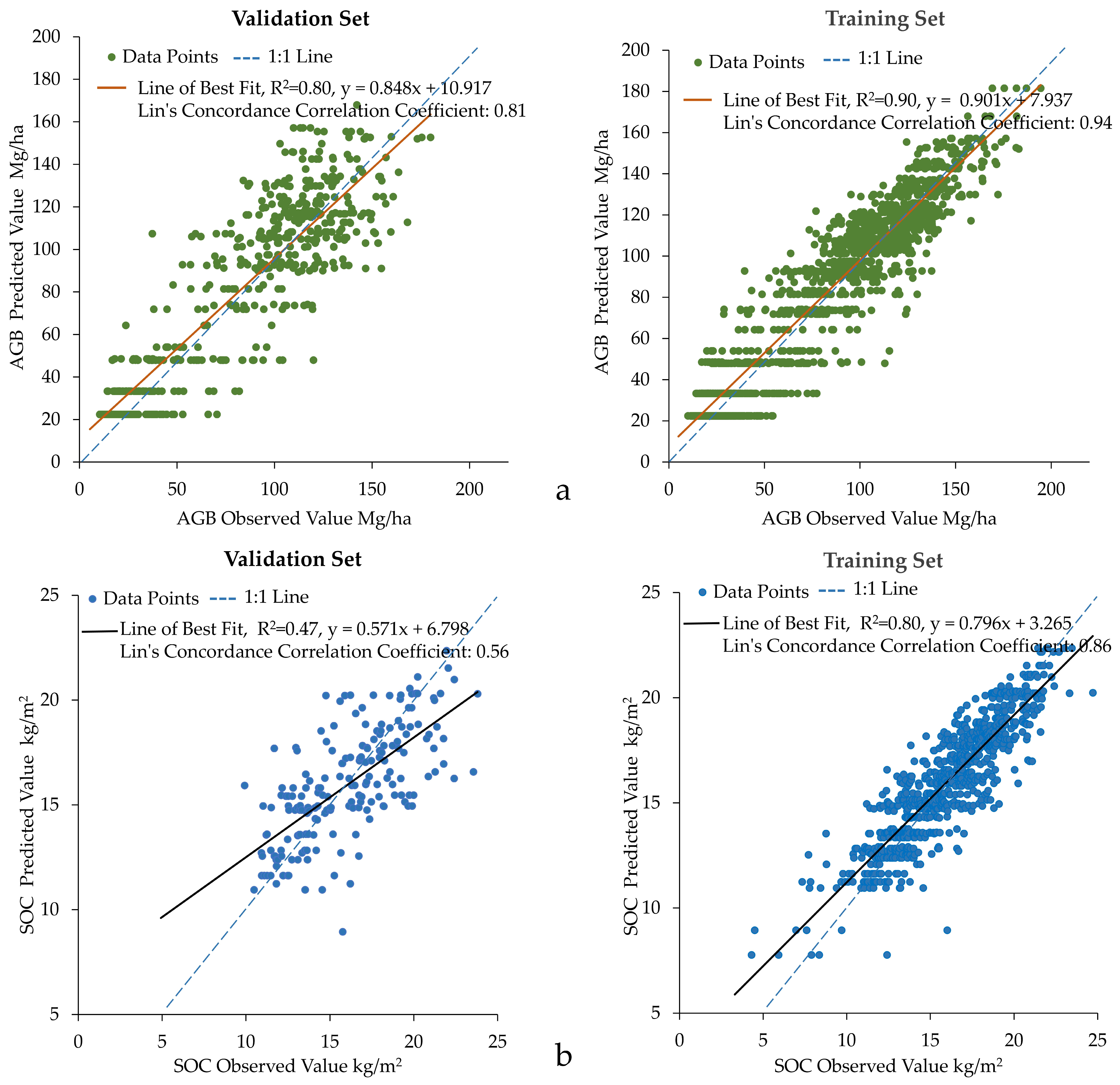
Figure 5a shows the relationship between predicted and observed values in the AGB training dataset and validation dataset. The AGB training dataset linear regression equation is predicted value = 0.901 × AGB observed value + 7.937, with an R2 of 0.90, RMSE of 14.20, and MAE of 10.86. The AGB validation data linear regression equation is predicted value = 0.860 × AGB observed value + 10.913, with an R2 of 0.80, RMSE of 20.49, and MAE of 15.52. This indicates that the model performs well in predicting AGB for both training and validation datasets, comparable to the Random Forest model. Figure 5b shows the relationship between predicted and observed values in the SOC training dataset. The linear regression equation is predicted value = 0.796 × SOC observed value + 3.265, with an R2 of 0.80, RMSE of 1.40, and MAE of 1.05. The SOC validation data linear regression equation is predicted value = 0.571 × SOC observed value + 6.798, with an R2 of 0.47, RMSE of 2.36, and MAE of 1.78. This indicates that the model has weak explanatory power for SOC predictions.
The horizontal grouping phenomenon in the scatter plot of the CART model, where multiple observed values correspond to the same predicted value, is an inherent product of the CART architecture, rooted in the algorithm’s piecewise constant prediction mechanism [44]. CART generates a binary tree structure through recursive partitioning and sets the predicted value of each leaf node as the arithmetic mean of the target variable of training samples within the node. This design leads to a stepwise discretization feature in model output. Even with parameter optimization to achieve finer-grained data partitioning, a single decision tree cannot generate continuously varying predicted values for samples with similar feature combinations.
Based on the R2, RMSE, and MAE of the training and validation datasets, comparing Random Forest, Gradient Boosting Decision Tree, and CART models, the model with a high R2 and low RMSE/MAE was selected. Finally, the AGB and SOC prediction values of the Random Forest model were determined as the data for subsequent analysis.

3.3. Importance of Environmental Variables

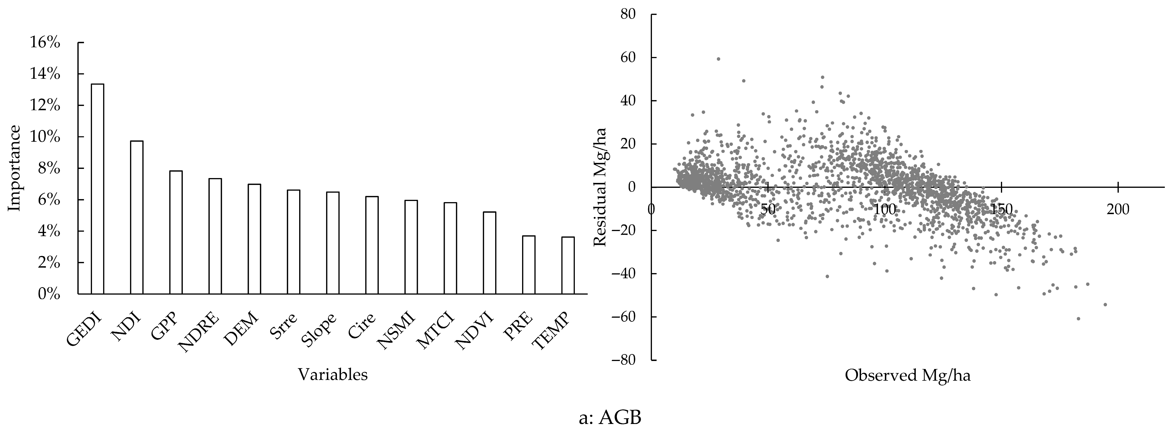
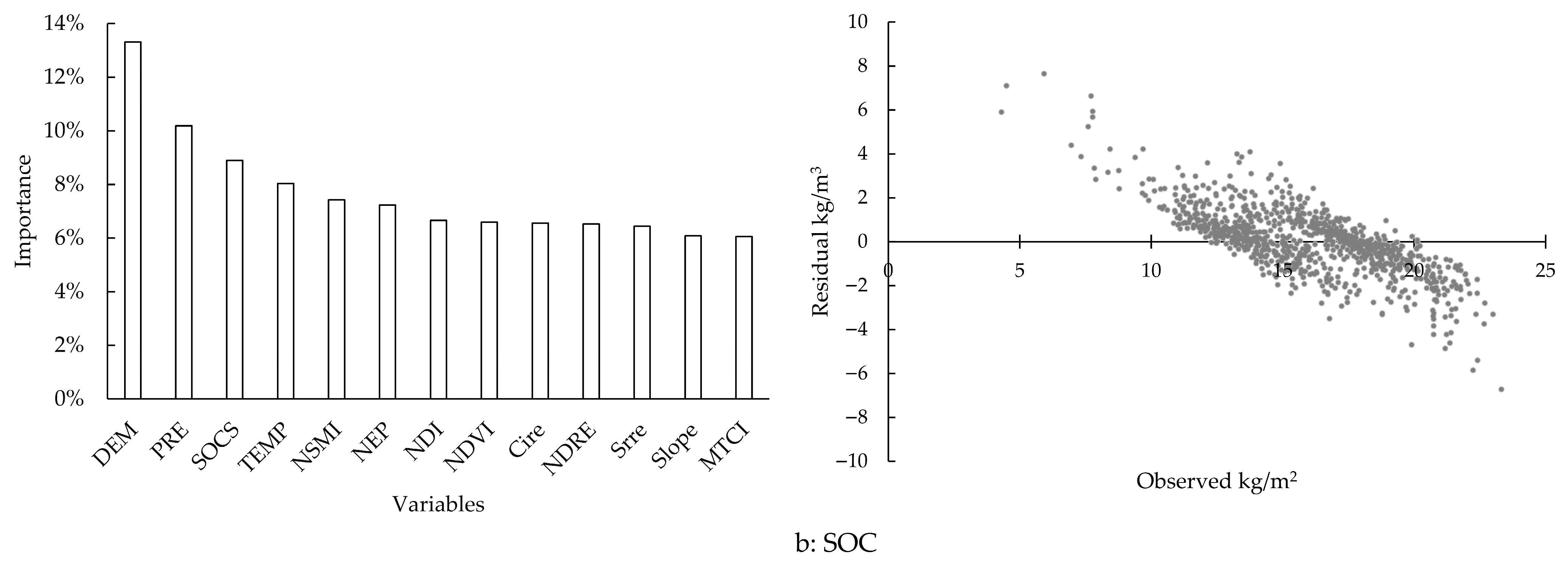
Based on the Random Forest model, the importance of environmental variables and residual characteristics of predicted values were analyzed (Figure 6). GEDI data contributed most significantly to AGB prediction (13%), highlighting the core role of LiDAR in parsing vegetation vertical structure. This was followed by radar-derived Normalized Difference Index (10%), Gross Primary Productivity (8%), and Red Edge Index (7%). Topographic variables (elevation, slope) and climate data (precipitation, temperature) indirectly affected the prediction results by regulating the vegetation growth environment. The AGB residual range was wide (−56 to +50 Mg/ha), but 68% of residuals were concentrated in the −20 to +20 Mg/ha interval, indicating high prediction stability for areas with AGB < 150 Mg/ha. Among environmental variables for SOC prediction, elevation (13%) and climate (precipitation 10%, temperature 8%) dominated SOC differences, followed by Soil Moisture Index (7%) and vegetation indices (NDVI, NDRE, Cire, NDI, NEP: 7%), with slope and MTCI contributing less (6%). The dominant role of elevation and precipitation variables reveals the environmental sensitivity of the soil carbon pool. The SOC residual range was −5.75 to +7.25 kg/m2, with 85% of residuals concentrated in −2 to +2 kg/m2. The clustering of points stems from the natural concentration of observed SOC values within specific ranges (e.g., >5 kg/m2) across the sampled ecosystems, driven by their inherent biophysical properties. In high-value SOC areas with soil organic carbon density > 15 kg/m2, the average residual was −0.59 kg/m2, while in areas < 15 kg/m3, the average residual was 0.92 kg/m2, reflecting smaller prediction errors for high-value SOC.

3.4. Distribution Characteristics of Carbon Storage

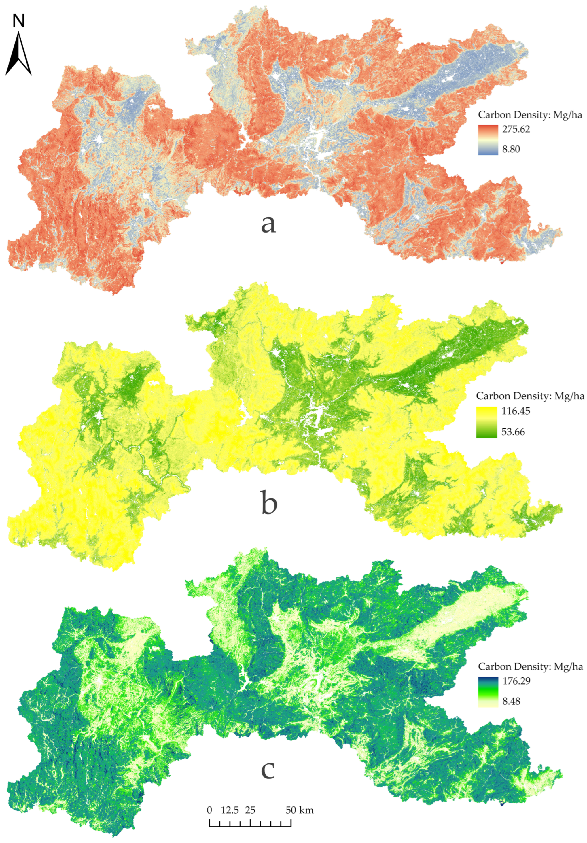
In 2022, the ecosystem carbon storage in the Nanling Mountains of Guangdong Province was 404 million tons, including 162 million tons of vegetation carbon storage (40%) and 242 million tons of soil carbon storage (60%). Forest ecosystems, accounting for 94.1% of the area, are the main ecosystems in the Nanling Mountains of Guangdong Province. The carbon storage of forest ecosystems was 391 million tons, accounting for 96.7%, making it the dominant carbon pool in the region. The ecosystem carbon density in the Nanling Mountains of Guangdong ranges from 8.80 Mg/ha to 275.62 Mg/ha, with soil carbon density ranging from 53.66 Mg/ha to 116.45 Mg/ha and vegetation carbon density ranging from 8.48 Mg/ha to 176.29 Mg/ha. High carbon density in the Nanling Mountains of Guangdong overlaps with high altitude, with 49.2% of carbon density >160 Mg/ha, of which 91.4% is in areas above 300 m altitude and 58.3% above 500 m altitude (Figure 7). Furthermore, 80% of carbon storage in the Nanling Mountains of Guangdong is located below 700 m altitude, while areas above 1000 m account for only 5.3%. In mountain valleys below 250 m altitude, carbon density is <100 Mg/ha, accounting for only 15.2% of carbon storage.

4. Discussion

(1)
Methodological Innovation and Applicability
Su, H et al. [49] and Wu, Y et al. [50] predicted the AGB in northern Guangdong Province, with R2 values of 0.81 and 0.69, respectively. In contrast, this study achieved an AGB prediction R2 of 0.87, representing improvements of approximately 7% and 26% over their results. For SOC, Tang, X et al. [51] reported R2 values of 0.35–0.46 for SOC prediction in subtropical Moso bamboo forests in China, while Yao, X et al. [52] obtained R2 values of 0.24–0.55 for SOC prediction in subtropical Masson pine forests in China. This study, however, achieved an SOC prediction R2 of 0.65, which fully highlights the significant advantages of the “optical-radar-topography-climate” multi-source collaborative framework constructed herein for carbon storage assessment in complex terrains. Optical remote sensing captures vegetation coverage dynamics through high-resolution vegetation indices but has data gaps in cloudy and rainy areas; radar data compensate for this shortcoming by penetrating vegetation canopies and resisting cloud interference. Especially in steep slope dense forest areas, it reduces the impact of surface roughness on signals and improves biomass inversion stability. GEDI LiDAR data significantly optimize biomass prediction in high-density vegetation areas by directly measuring vegetation vertical structure, but its spatial coverage discontinuity and orbital gaps may introduce systematic errors in extrapolated predictions for some areas. Combining optical, radar, topography, and climate data can comprehensively characterize the driving mechanisms of SOC distribution. For example, the Soil Moisture Index improves the detection capability of underground organic matter distribution, while topographic variables capture SOC redistribution driven by erosion. Different from traditional regression models, Random Forest reduces overfitting risk through bootstrap aggregation and random feature selection, especially suitable for high-heterogeneity landscapes like the Nanling Mountains. The overfitting of Gradient Boosting Decision Tree in the training set but insufficient validation set stability led to its abandonment, confirming the argument of Random Forest robustness in multi-source data regression tasks. The discrete prediction problem of CART highlights the inherent defect of single decision trees in continuous variable inversion. In addition, compared with traditional single-source remote sensing models, the multi-source collaborative framework breaks through the limitations of single technology through data complementarity. The parallel computing capability of the GEE platform supports fast processing of PB-level data, making large-scale, high-resolution carbon storage dynamic monitoring possible, providing an expandable template for high-resolution carbon storage mapping in mountain ecosystems.
(2)
The Role of Multi-source Data
The preeminent contribution of GEDI LiDAR highlights its irreplaceable role in quantifying vertical canopy architecture—a critical structural parameter often obscured by optical sensors in dense forest canopies. The synergistic integration of radar and optical remote sensing proved particularly indispensable in humid, topographically complex regions, where L-band radar data mitigated optical limitations by penetrating persistent cloud cover and dense vegetation layers to capture sub-canopy structural signatures. Additionally, elevation and precipitation emerged as joint regulators of SOC patterns, operating through dual mechanisms: erosion-mediated carbon redistribution in mountainous terrain and moisture-dependent modulation of microbial decomposition rates. These findings underscore the need for multi-source data fusion—coupled with variable-specific optimization—to address the spatiotemporal heterogeneity of montane ecosystems. Such an approach advances high-resolution carbon storage mapping, thereby enabling climate-resilient land management strategies tailored to complex topographic landscapes.
(3)
Management Implications
The spatial differentiation law of carbon storage revealed in this study provides a key decision-making basis for the construction of Nanling National Park and ecosystem protection and carbon sink function improvement. The 300–700 m altitude area, with a carbon density of up to 160 Mg/ha, accounts for 49.2% of the regional total carbon storage and is the core carbon sink area, which can be prioritized as a core protection area for inclusion in Nanling National Park. For this area, carbon accumulation rates can be improved through artificial forest tending and natural forest closure. In low-altitude valleys (<250 m), farmland carbon density is <100 Mg/ha, and surface SOC can be increased by 15–30% through conservation tillage and organic fertilizer application. To improve the spatiotemporal continuity of carbon storage estimation, fixed monitoring plots can be set up in typical sample areas and dynamically calibrated combined with remote sensing inversion results. As a critical ecological barrier in Guangdong Province, the Nanling Mountains play a pivotal role in offsetting carbon emissions from urban agglomerations through their robust carbon sink function. Beyond this regional significance, our proposed “optical-radar-topography-climate” integrated framework provides robust support for global carbon monitoring in subtropical mountain ecosystems, thereby facilitating the quantification of Nationally Determined Contributions under the Paris Agreement. Equipped with 30 m high-resolution data, this framework enables precise tracking of carbon sink increments—directly supporting China’s commitments to reach carbon peak by 2030 and achieve carbon neutrality by 2060. To fully leverage these ecological and scientific insights, it is imperative to clarify carbon sink increment targets and advance the implementation of ecological compensation mechanisms through carbon trading markets, thus translating carbon sink value into tangible incentives for sustainable management.
(4)
Limitations and Future Directions
Although this study has made progress in multi-source data fusion and model construction, the following limitations remain. The prediction of soil carbon storage is limited by the lack of pH, clay content, and agricultural management data, which is the reason for the difficulty in improving soil carbon prediction accuracy. For example, high-altitude acidic soils promote SOC accumulation by inhibiting decomposition, but this mechanism is not quantified in the model. The short-term impact of extreme climate events is not included, which may lead to accelerated soil carbon decomposition, but the model does not simulate the nonlinear effect of drought events. The multi-source collaborative framework and high-precision carbon storage distribution map constructed in this study provide key regional parameters for global carbon cycle models. Soil carbon accounts for 60% of regional total carbon storage, highlighting the contribution of mountain ecosystem soil carbon pools to the global carbon balance. This study not only provides technical support for carbon management in the Nanling Mountains but also offers a case reference for carbon storage assessment in complex terrain areas worldwide.

5. Conclusions

Based on the GEE platform, this study integrates multi-source remote sensing data (Sentinel-1/2, ALOS, GEDI, MODIS) and environmental variables, using machine learning algorithms to achieve a comprehensive assessment of carbon storage in the Nanling Mountains of Guangdong Province, supporting boundary optimization of the Nanling National Park and ecosystem carbon sink management practices. The core conclusions are as follows:
(1) By comparing the performance of Random Forest, Gradient Boosting Decision Tree, and CART algorithms, Random Forest was established as the optimal prediction algorithm. Its dual randomness effectively suppresses overfitting in complex terrain, in particular showing more stability in SOC prediction. The multi-feature fusion model of “optical-radar-LiDAR-topography-climate” performs best, with vegetation biomass and soil carbon prediction accuracies higher than single data source and optical/radar fusion data, especially for SOC. GEDI data become a key variable for biomass prediction by capturing vegetation vertical structure; precipitation and topographic variables optimize soil carbon estimation by regulating decomposition rates.
(2) The total carbon storage in the Nanling Mountains is 404 million tons, of which soil carbon accounts for 60% (242 million tons) and vegetation carbon accounts for 40% (162 million tons). High carbon density areas (>160 Mg C/ha) are concentrated in the mid-altitude gentle slope zone (300–700 m), accounting for 49.2% of the regional total carbon storage; low-altitude valleys (<250 m) are affected by agriculture and urbanization, with carbon density <100 Mg C/ha.
(3) Carbon storage distribution is dominated by the feedback mechanism of terrain/climate/vegetation. Precipitation and temperature affect carbon accumulation by regulating vegetation productivity and soil organic carbon decomposition rate; land use types (forest, farmland) directly determine carbon allocation patterns, with evergreen broad-leaved forest carbon density being significantly higher than shrubland and farmland.

Author Contributions

W.W.: writing—original draft, software, visualization, and methodology. X.C.: resources, funding acquisition. X.M.: project administration, and writing—review and editing. Y.Z.: data curation. L.T.: software, visualization. J.C.: validation. All authors have read and agreed to the published version of the manuscript.

Funding

This work was supported by the National Key R&D Program of China [grant number 2023YFD1900100], the Guangdong Basic and Applied Basic Research Foundation [grant number 2023A1515011736], and the Shaoguan Science and Technology Plan Project [grant number 220531134531827].

Data Availability Statement

The code for this study is publicly available on the Google Earth Engine platform: https://code.earthengine.google.com/742d6be82f4738be557309693a687eb9 (accessed on 24 June 2025, requires a GEE account to access and execute). All carbon storage results are openly accessible on Google Drive (https://drive.google.com/drive/folders/13pzHulxU4I6uDYvlGq0Ynd-3B9S8lPSZ?usp=drive_link (accessed on 24 June 2025)).

Acknowledgments

The authors greatly appreciate the constructive comments of the reviewers and editors.

Conflicts of Interest

The authors declare no conflicts of interest.

References

  1. Pan, Y.; Birdsey, R.A.; Fang, J.; Houghton, R.; Kauppi, P.E.; Kurz, W.A.; Phillips, O.L.; Shvidenko, A.; Lewis, S.L.; Canadell, J.G.; et al. A large and persistent carbon sink in the world’s forests. Science 2011, 333, 988–993. [Google Scholar] [CrossRef] [PubMed]
  2. Bonan, G.B. Forests and climate change: Forcings, feedbacks, and the climate benefits of forests. Science 2008, 320, 1444–1449. [Google Scholar] [CrossRef] [PubMed]
  3. Gatti, L.V.; Basso, L.S.; Miller, J.B.; Gloor, M.; Gatti Domingues, L.; Cassol, H.L.; Tejada, G.; Aragão, L.E.; Nobre, C.; Peters, W.; et al. Amazonia as a carbon source linked to deforestation and climate change. Nature 2021, 595, 388–393. [Google Scholar] [CrossRef] [PubMed]
  4. Tang, X.; Zhao, X.; Bai, Y.; Tang, Z.; Wang, W.; Zhao, Y.; Wan, H.; Xie, Z.; Shi, X.; Wu, B.; et al. Carbon pools in China’s terrestrial ecosystems: New estimates based on an intensive field survey. Proc. Natl. Acad. Sci. USA 2018, 115, 4021–4026. [Google Scholar] [CrossRef]
  5. Huang, L.; Yuan, L.; Xia, Y.; Yang, Z.; Luo, Z.; Yan, Z.; Li, M.; Yuan, J. Landscape ecological risk analysis of subtropical vulnerable mountainous areas from a spatiotemporal perspective: Insights from the Nanling Mountains of China. Ecol. Indic. 2023, 154, 110883. [Google Scholar] [CrossRef]
  6. Issa, S.; Dahy, B.; Ksiksi, T.; Saleous, N. A Review of Terrestrial Carbon Assessment Methods Using Geo-Spatial Technologies with Emphasis on Arid Lands. Remote Sens. 2020, 12, 2008. [Google Scholar] [CrossRef]
  7. Houghton, R.A.; Nassikas, A.A. Global and regional fluxes of carbon from land use and land cover change 1850–2015. Glob. Biogeochem. Cycles 2017, 31, 456–472. [Google Scholar] [CrossRef]
  8. Zhu, Z.; Wang, S.; Woodcock, C.E. Improvement and expansion of the Fmask algorithm: Cloud, cloud shadow, and snow detection for Landsats 4–7, 8, and Sentinel 2 images. Remote Sens. Environ. 2015, 159, 269–277. [Google Scholar] [CrossRef]
  9. Musthafa, M.; Singh, G. Improving forest above-ground biomass retrieval using multi-sensor L-and C-band SAR data and multi-temporal spaceborne LiDAR data. Front. For. Glob. Change 2022, 5, 822704. [Google Scholar] [CrossRef]
  10. Paustian, K.; Ravindranath, N.H.; Amstel, A.V. 2006 IPCC Guidelines for National Greenhouse Gas Inventories; International Panel on Climate Change: Geneva, Switzerland, 2006. [Google Scholar]
  11. Baccini, A.G.S.J.; Goetz, S.J.; Walker, W.S.; Laporte, N.T.; Sun, M.; Sulla-Menashe, D.; Hackler, J.; Beck, P.S.A.; Dubayah, R.; Friedl, M.A.; et al. Estimated carbon dioxide emissions from tropical deforestation improved by carbon-density maps. Nat. Clim. Change 2012, 2, 182–185. [Google Scholar] [CrossRef]
  12. Forkel, M.; Drüke, M.; Thurner, M.; Dorigo, W.; Schaphoff, S.; Thonicke, K.; von Bloh, W.; Carvalhais, N. Constraining modelled global vegetation dynamics and carbon turnover using multiple satellite observations. Sci. Rep. 2019, 9, 18757. [Google Scholar] [CrossRef] [PubMed]
  13. Zhu, Z.; Wulder, M.A.; Roy, D.P.; Woodcock, C.E.; Hansen, M.C.; Radeloff, V.C.; Healey, S.P.; Schaaf, C.; Hostert, P.; Strobl, P.; et al. Benefits of the free and open Landsat data policy. Remote Sens. Environ. 2019, 224, 382–385. [Google Scholar] [CrossRef]
  14. Dubayah, R.; Blair, J.B.; Goetz, S.; Fatoyinbo, L.; Hansen, M.; Healey, S.; Hofton, M.; Hurtt, G.; Kellner, J.; Luthcke, S.; et al. The Global Ecosystem Dynamics Investigation: High-resolution laser ranging of the Earth’s forests and topography. Sci. Remote Sens. 2020, 1, 100002. [Google Scholar] [CrossRef]
  15. Neuenschwander, A.; Pitts, K. The ATL08 land and vegetation product for the ICESat-2 Mission. Remote Sens. Environ. 2019, 221, 247–259. [Google Scholar] [CrossRef]
  16. Saatchi, S.; Longo, M.; Xu, L.; Yang, Y.; Abe, H.; André, M.; Aukema, J.E.; Carvalhais, N.; Cadillo-Quiroz, H.; Cerbu, G.A.; et al. Detecting vulnerability of humid tropical forests to multiple stressors. One Earth 2021, 4, 988–1003. [Google Scholar] [CrossRef]
  17. Duncanson, L.; Kellner, J.R.; Armston, J.; Dubayah, R.; Minor, D.M.; Hancock, S.; Healey, S.P.; Patterson, P.L.; Saarela, S.; Marselis, S.; et al. Aboveground biomass density models for NASA’s Global Ecosystem Dynamics Investigation (GEDI) lidar mission. Remote Sens. Environ. 2022, 270, 112845. [Google Scholar] [CrossRef]
  18. Yang, H.; Qin, Z.; Shu, Q.; Xu, L.; Yu, J.; Luo, S.; Wu, Z.; Xia, C.; Yang, Z. Estimation of Above-Ground Biomass for Dendrocalamus Giganteus Utilizing Spaceborne LiDAR GEDI Data. IEEE J. Sel. Top. Appl. Earth Obs. Remote Sens. 2025, 18, 5271–5286. [Google Scholar] [CrossRef]
  19. Yu, Y.; Saatchi, S. Sensitivity of L-band SAR backscatter to aboveground biomass of global forests. Remote Sens. 2016, 8, 522. [Google Scholar] [CrossRef]
  20. Berninger, A.; Lohberger, S.; Stängel, M.; Siegert, F. SAR-Based Estimation of Above-Ground Biomass and Its Changes in Tropical Forests of Kalimantan Using L- and C-Band. Remote Sens. 2018, 10, 831. [Google Scholar] [CrossRef]
  21. Yan, X.; Li, J.; Smith, A.R.; Yang, D.; Ma, T.; Su, Y.; Shao, J. Evaluation of machine learning methods and multi-source remote sensing data combinations to construct forest above-ground biomass models. Int. J. Digit. Earth 2023, 16, 4471–4491. [Google Scholar] [CrossRef]
  22. Ali, H.; Mohammadi, J.; Shataee Jouibary, S. Deep and machine learning prediction of forest above-ground biomass using multi-source remote sensing data in coniferous planted forests in Iran. Eur. J. For. Res. 2024, 143, 1731–1745. [Google Scholar] [CrossRef]
  23. Wang, X.; Liu, C.; Lv, G.; Xu, J.; Cui, G. Integrating Multi-Source Remote Sensing to Assess Forest Aboveground Biomass in the Khingan Mountains of North-Eastern China Using Machine-Learning Algorithms. Remote Sens. 2022, 14, 1039. [Google Scholar] [CrossRef]
  24. Singha, C.; Chandra Swain, K.; Sahoo, S.; Fadhil Al-Quraishi, A.M.; Omeiza Alao, J.; Almohamad, H.; Fatahalla Mohamed Ahmed, M.; Ghassan Abdo, H. Predicting forest above-ground biomass using SAR imagery and GEDI data through machine learning in GEE cloud. For. Sci. Technol. 2025, 21, 187–206. [Google Scholar] [CrossRef]
  25. Tamiminia, H.; Salehi, B.; Mahdianpari, M.; Quackenbush, L.; Adeli, S.; Brisco, B. Google Earth Engine for geo-big data applications: A meta-analysis and systematic review. ISPRS J. Photogramm. Remote Sens. 2020, 164, 152–170. [Google Scholar] [CrossRef]
  26. Zurqani, H.A. A multi-source approach combining GEDI LiDAR, satellite data, and machine learning algorithms for estimating forest aboveground biomass on Google Earth engine platform. Ecol. Inform. 2025, 86, 103052. [Google Scholar] [CrossRef]
  27. Hengl, T.; Mendes de Jesus, J.; Heuvelink, G.B.; Ruiperez Gonzalez, M.; Kilibarda, M.; Blagotić, A.; Shangguan, W.; Wright, M.N.; Geng, X.; Bauer-Marschallinger, B.; et al. SoilGrids250m: Global gridded soil information based on machine learning. PLoS ONE 2017, 12, 0169748. [Google Scholar] [CrossRef]
  28. Viscarra Rossel, R.A.; Lee, J.; Behrens, T.; Luo, Z.; Baldock, J.; Richards, A. Continental-scale soil carbon composition and vulnerability modulated by regional environmental controls. Nat. Geosci. 2019, 12, 547–552. [Google Scholar] [CrossRef]
  29. Poggio, L.; De Sousa, L.M.; Batjes, N.H.; Heuvelink, G.B.; Kempen, B.; Ribeiro, E.; Rossiter, D. SoilGrids 2.0: Producing soil information for the globe with quantified spatial uncertainty. Soil 2021, 7, 217–240. [Google Scholar] [CrossRef]
  30. Vaudour, E.; Gomez, C.; Fouad, Y.; Lagacherie, P. Sentinel-2 image capacities to predict common topsoil properties of temperate and Mediterranean agroecosystems. Remote Sens. Environ. 2019, 223, 21–33. [Google Scholar] [CrossRef]
  31. Schillaci, C.; Acutis, M.; Lombardo, L.; Lipani, A.; Fantappie, M.; Märker, M.; Saia, S. Spatio-temporal topsoil organic carbon mapping of a semi-arid Mediterranean region: The role of land use, soil texture, topographic indices and the influence of remote sensing data to modelling. Sci. Total Environ. 2017, 601, 821–832. [Google Scholar] [CrossRef]
  32. Zhou, T.; Geng, Y.; Ji, C.; Xu, X.; Wang, H.; Pan, J.; Bumberger, J.; Haase, D.; Lausch, A. Prediction of soil organic carbon and the C: N ratio on a national scale using machine learning and satellite data: A comparison between Sentinel-2, Sentinel-3 and Landsat-8 images. Sci. Total Environ. 2021, 755, 142661. [Google Scholar] [CrossRef]
  33. Ho, V.H.; Morita, H.; Ho, T.H.; Bachofer, F.; Nguyen, T.T. Comparison of geostatistics, machine learning algorithms, and their hybrid approaches for modeling soil organic carbon density in tropical forests. J. Soils Sediments 2025, 25, 1554–1577. [Google Scholar] [CrossRef]
  34. Wu, T.; Luo, J.; Dong, W.; Sun, Y.; Xia, L.; Zhang, X. Geo-object-based soil organic matter mapping using machine learning algorithms with multi-source geo-spatial data. IEEE J. Sel. Top. Appl. Earth Obs. Remote Sens. 2019, 12, 1091–1106. [Google Scholar] [CrossRef]
  35. Lei, S.; Zhou, P.; Lin, J.; Tan, Z.; Huang, J.; Yan, P.; Chen, H. Spatiotemporal Variation in Carbon and Water Use Efficiency and Their Influencing Variables Based on Remote Sensing Data in the Nanling Mountains Region. Remote Sens. 2025, 17, 648. [Google Scholar] [CrossRef]
  36. Peng, S. 1-km Monthly Precipitation Dataset for China (1901–2023); National Tibetan Plateau/Third Pole Environment Data Center: Beijing, China, 2020; Available online: https://data.tpdc.ac.cn/en/data/faae7605-a0f2-4d18-b28f-5cee413766a2 (accessed on 24 June 2025).
  37. Zhang, X.; Zhao, T.; Xu, H.; Liu, W.; Wang, J.; Chen, X.; Liu, L. GLC_FCS30D: The first global 30 m land-cover dynamics monitoring product with a fine classification system for the period from 1985 to 2022 generated using dense-time-series Landsat imagery and the continuous change-detection method. Earth Syst. Sci. Data. 2024, 16, 1353–1381. [Google Scholar] [CrossRef]
  38. Zhu, M.; Feng, Q.; Qin, Y.; Cao, J.; Zhang, M.; Liu, W.; Deo, R.C.; Zhang, C.; Li, R.; Li, B. The role of topography in shaping the spatial patterns of soil organic carbon. Catena 2019, 176, 296–305. [Google Scholar] [CrossRef]
  39. Hegazi, E.H.; Samak, A.A.; Yang, L.; Huang, R.; Huang, J. Prediction of Soil Moisture Content from Sentinel-2 Images Using Convolutional Neural Network (CNN). Agronomy 2023, 13, 656. [Google Scholar] [CrossRef]
  40. Sims, D.A.; Gamon, J.A. Relationships between leaf pigment content and spectral reflectance across a wide range of species, leaf structures and developmental stages. Remote Sens. Environ. 2002, 81, 337–354. [Google Scholar] [CrossRef]
  41. Pei, Z.Y.; Ouyang, H.; Zhou, C.P.; Xu, X.L. Carbon Balance in an Alpine Steppe in the Qinghai-Tibet Plateau. J. Integr. Plant Biol. 2009, 51, 521–526. [Google Scholar] [CrossRef]
  42. Breiman, L. Random Forests. Mach. Learn. 2001, 45, 5–32. [Google Scholar] [CrossRef]
  43. Cutler, D.R.; Edwards, T.C., Jr.; Beard, K.H.; Cutler, A.; Hess, K.T.; Gibson, J.; Lawler, J.J. Random forests for classification in ecology. Ecology 2007, 88, 2783–2792. [Google Scholar] [CrossRef]
  44. Friedman, J.H. Greedy function approximation: A gradient boosting machine. Ann. Stat. 2001, 29, 1189–1232. Available online: http://www.jstor.org/stable/2699986 (accessed on 24 June 2025). [CrossRef]
  45. Natekin, A.; Knoll, A. Gradient boosting machines, a tutorial. Front. Neurorobotics 2013, 7, 21. [Google Scholar] [CrossRef]
  46. Loh, W.Y. Classification and regression trees. Wiley Interdiscip. Rev. Data Min. Knowl. Discov. 2011, 1, 14–23. [Google Scholar] [CrossRef]
  47. Fan, Q.; Jiang, Y.; Wang, Y.; Fan, G. Forest Carbon Storage Dynamics and Influencing Factors in Southeastern Tibet: GEE and Machine Learning Analysis. Forests 2025, 16, 825. [Google Scholar] [CrossRef]
  48. Intergovernmental Panel on Climate Change. 2019 Refinement to the 2006 IPCC Guidelines for National Greenhouse Gas Inventories. IPCC. 2019. Available online: http://www.ipcc.ch/report/2019-refinement-to-the-2006-ipcc-guidelines-for-national-greenhouse-gas-inventories/ (accessed on 24 June 2025).
  49. Su, H.; Shen, W.; Wang, J.; Ali, A.; Li, M. Machine learning and geostatistical approaches for estimating aboveground biomass in Chinese subtropical forests. For. Ecosyst. 2020, 7, 64. [Google Scholar] [CrossRef]
  50. Wu, Y.; Chen, Y.; Tian, C.; Yun, T.; Li, M. Estimation of Subtropical Forest Aboveground Biomass Using Active and Passive Sentinel Data with Canopy Height. Remote Sens. 2025, 17, 2509. [Google Scholar] [CrossRef]
  51. Tang, X.; Xia, M.; Pérez-Cruzado, C.; Guan, F.; Fan, S. Spatial distribution of soil organic carbon stock in Moso bamboo forests in subtropical China. Sci. Rep. 2017, 7, 42640. [Google Scholar] [CrossRef] [PubMed]
  52. Yao, X.; Yu, K.; Deng, Y.; Zeng, Q.; Lai, Z.; Liu, J. Spatial distribution of soil organic carbon stocks in Masson pine (Pinus massoniana) forests in subtropical China. Catena 2019, 178, 189–198. [Google Scholar] [CrossRef]
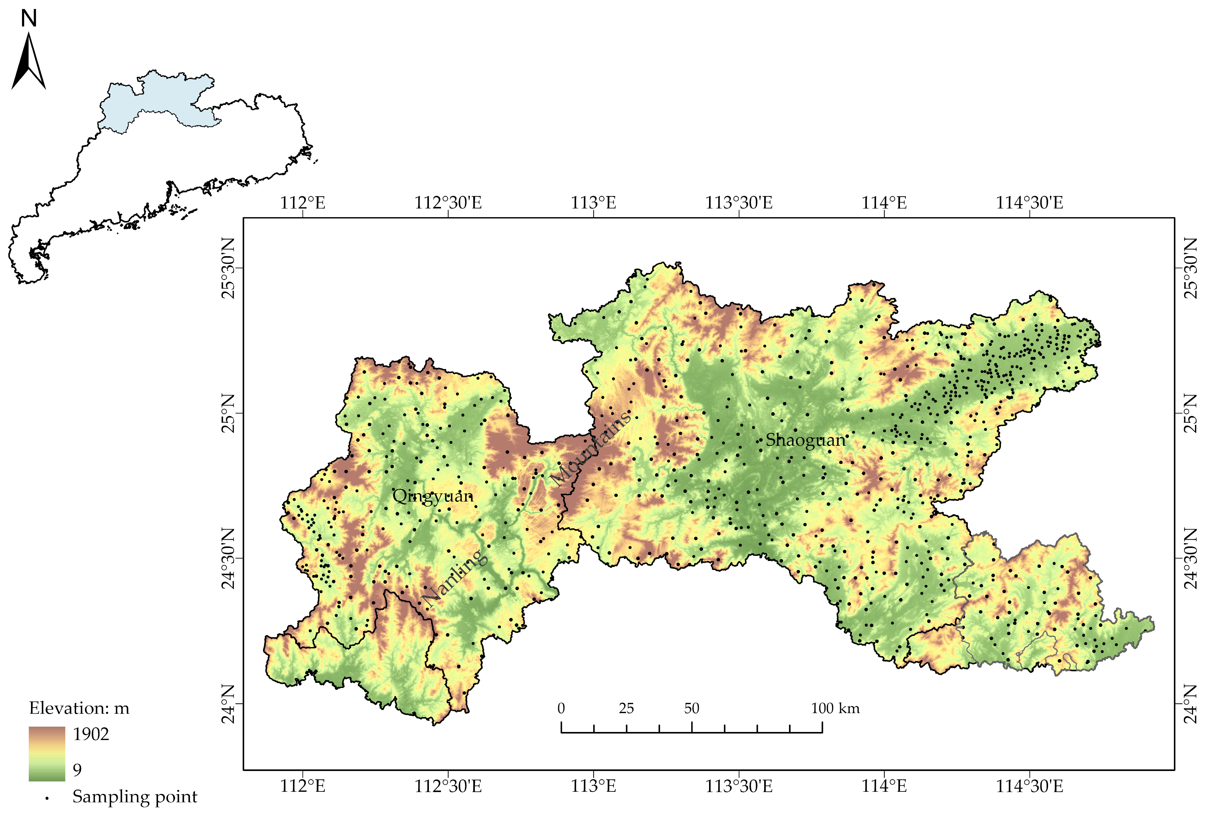
Figure 1. Terrain and sampling point distribution in the Nanling Mountains, Guangdong Province (sampling density correlates with ecosystem complexity (highest in forests), improving local prediction accuracy; DEM from 30 m SRTM data).
Atmosphere 16 00954 g001
Figure 2. Roadmap for research.
Atmosphere 16 00954 g002
Figure 3. Random Forest training set and validation set of AGB (a) and SOC (b).
Atmosphere 16 00954 g003
Figure 4. Gradient Boosting Decision Tree training set and validation set of AGB (a) and SOC (b).
Atmosphere 16 00954 g004
Figure 5. CART training set and validation set of AGB (a) and SOC (b).
Atmosphere 16 00954 g005
Figure 6. Environmental variables and residual distribution.
Atmosphere 16 00954 g006aAtmosphere 16 00954 g006b
Figure 7. Spatial distribution of carbon density components (a) total carbon density, (b) soil organic carbon density, (c) vegetation carbon density; high-density areas (>160 Mg C/ha) concentrate in 300–700 m elevation, overlapping with forests.
Atmosphere 16 00954 g007
Table 1. Data and sources.
DataResolutionSource
Sentinel-210 m/20 mHarmonized Sentinel-2 MSI, Union/ESA/Copernicus
Sentinel-110 mSentinel-1 SAR GRD, Union/ESA/Copernicus
ALOS25 mGlobal PALSAR-2/PALSAR Yearly Mosaic, version 2, JAXA EORC
MODIS500 mNASA LP DAAC at the USGS EROS Center
DEM30 mUSGS/SRTMGL1_003
GEDI25 mGridded Aboveground Biomass Density, USGS LP DAAC
Soil type1 kmHWSD2.0, https://openknowledge.fao.org/handle/20.500.14283/cc3823en (accessed on 24 June 2025)
Temperature1 kmPeng, S. (2020), https://data.tpdc.ac.cn/en/data/faae7605-a0f2-4d18-b28f-5cee413766a2 (accessed on 24 June 2025) [36]
Precipitation1 km
Land use30 mGLC-FCS30D, Zhang et al., 2024 [37]
Field sampling data Soil sampling and vegetation sampling
Table 2. Environmental variables and calculation methods.
TypeVariablesFormula
Optical Remote SensingNormalized Difference Vegetation Index (NDVI)(NIR − Red)/(NIR + Red) [26]
NIR: Near Infrared Band 1; Red: Red Band
Normalized Difference Red Edge Index (NDRE)(RedEdge2 − RedEdge1)/RedEdge2 + RedEdge1) [26]
RedEdge1/2: Red Edge Band 1/2
Normalized Soil Moisture Index (NSMI)(SWIR − NIR)/(SWIR + NIR) [39]
SWIR: Shortwave Infrared Band
Chlorophyll Index Red Edge (CIRE)NIR/RedEdge1 − 1 [40]
Simple Ratio Red Edge (SRRE)RedEdge3/RedEdge1 [40]
MERIS Terrestrial Chlorophyll Index (MTCI)(RedEdge2 − RedEdge1)/(RedEdge1 − Red) [26]
Gross Primary Productivity (GPP)
Net Primary Productivity (NPP)
Net Ecosystem Productivity (NEP)NPP-R0 [41], R0: Heterotrophic Respiration
R 0 = 0.22 × e 0.0913 × T + ln 0.3145 × P + 1 × 30 × 46.5 %
T: Temperature, P: Precipitation
Radar Remote SensingNormalized Difference Index (NDI)Log(10 × VV × VH) [19,26]
VV: Vertical-Vertical, VH: Vertical-Horizontal
Global Ecosystem Dynamics Investigation (GEDI)
TopographyDEM, Slop
ClimatePrecipitation (PRE), Temperature (TEMP)
OthersLand Use/Land Cover (LULC)
Table 3. Environmental variables for AGB and SOC prediction.
TypeVariables
AGBNDVI, NDRE, NSMI, SRRE, CIRE, MTCI, NDI, GEDI, DEM, Slope, GPP, TEMP, PRE
SOCNDVI, NDRE, NSMI, SRRE, CIRE, MTCI, NDI, DEM, Slope, NEP, TEMP, PRE
Table 4. Performance of AGB and SOC prediction with multi-source data.
ModelTypeR2RMSE (Mg/ha, kg/m2)MAE (Mg/ha, kg/m 2)
Optical remote sensingAGB0.7921.0315.66
SOC0.312.612.01
Optical/radar fusionAGB0.8517.1512.91
SOC0.402.401.82
Optical/radar fusion combined with terrain and climateAGB0.8716.2912.39
SOC0.651.921.50
Disclaimer/Publisher’s Note: The statements, opinions and data contained in all publications are solely those of the individual author(s) and contributor(s) and not of MDPI and/or the editor(s). MDPI and/or the editor(s) disclaim responsibility for any injury to people or property resulting from any ideas, methods, instructions or products referred to in the content.